SUBMITTED TO
THE DEPARTMENT OF STATISTICS OF THE UNIVERSITY OF DORTMUND
IN FULFILMENT OF
THE REQUIREMENTS FOR THE DEGREE OF DOCTOR OF NATURAL SCIENCES
BY
REGINALD NII OTOO ODAI FROM GHANA
DORTMUND 2003
Supervisor: Prof. Dr. Wolfgang Urfer Co-Supervisor: PD Dr. Jürgen Groß Date of the oral examination: July 29, 2003
THE USE OF THE CORRELATED WEIBULL AND LOGISTIC REGRESSION MODELS IN EPIDEMIOLOGY
ABSTRACT
An important factor in the analysis of family data is the dependence structure. In order to incorporate dependence within families into regression models, Bonney (1998) introduced the disposition model for the analysis of correlated binary data. In this work, the disposition model has been extended to allow for situations where quaternary-group dispositions are required. Estimation procedures for the correlated Weibull and logistic regression models have been provided for the non-nested and nested disposition models.
The correlated Weibull regression model was contrasted with the correlated logistic regression model. The results showed that both regression models were useful in explaining the familial aggregation of oesophageal cancer. The correlated logistic regression model fitted the oesophageal cancer data better than the correlated Weibull regression model. Furthermore, the correlated logistic regression model was computationally more attractive than the correlated Weibull regression model. The implications of higher level nesting of the disposition model in relation to the dimension of the parameter space have been examined and the performance of the disposition model compared to that of Cox’s model using breast cancer data. It has been observed that the disposition model has a very large number of unknown parameters, and is therefore limited by the method of estimation used. In the case of the maximum likelihood method, reasonable estimates are obtained if the number of parameters in the model is at most nine. This corresponds to about four to seven covariates.
Since each covariate in Cox’s model provides a parameter, it is possible to include more covariates in the regression analysis. On the other hand, as opposed to Cox’s model, the disposition model is fitted with parameters to capture aggregation in families, if there should be any. The choice of a particular model should therefore depend on the available data set and the purpose of the statistical analysis.
CONTENTS
ABSTRACT ...iii
CONTENTS ... iv
ACKNOWLEDGEMENTS ... vi
1 Background and literature review ... 1
1.1 Introduction ... 1
1.2 Review of correlated regression models ... 3
1.3 Motivation... 6
2 The standard Weibull distribution... 7
3 Cox’s regression model... 12
3.1 The model... 12
3.2 Parameter estimation ... 13
4 Introduction of the non-nested disposition model... 16
5 Extensions of the disposition model ... 21
5.1 First level nesting ... 21
5.2 Second level nesting... 26
6 Inference... 33
6.6 Parameter estimation for the non-nested disposition model ... 33
6.2 Parameter estimation for the first level nesting... 37
6.3 Parameter estimation for the second level nesting ... 42
6.4 Properties of the score function... 48
6.5 Tests of independence ... 59
6.6 Comparison of model fit ... 61
7 Application to real data sets ... 62
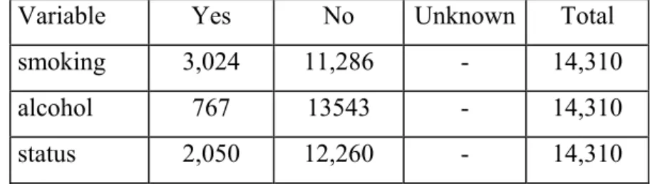
7.1 Description of the data sets ... 62
7.2 Analysis of the oesophageal cancer data... 64
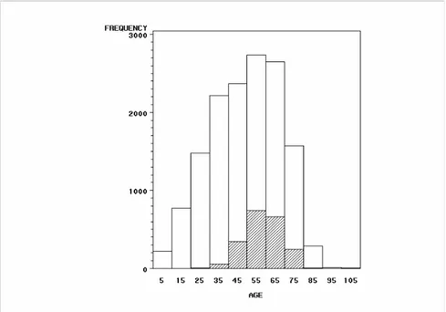
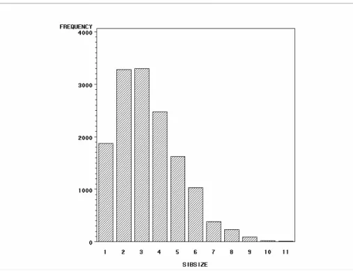
7.2.1 Descriptive analysis... 64
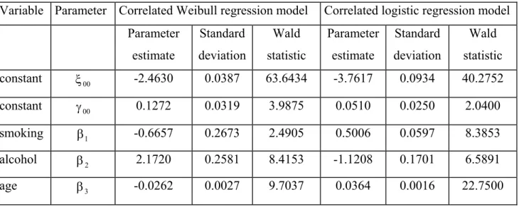
7.2.2 Model for the non-nested disposition model... 65
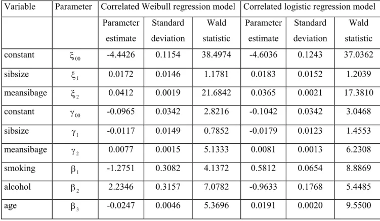
7.2.3 Model for the first level nesting ... 68
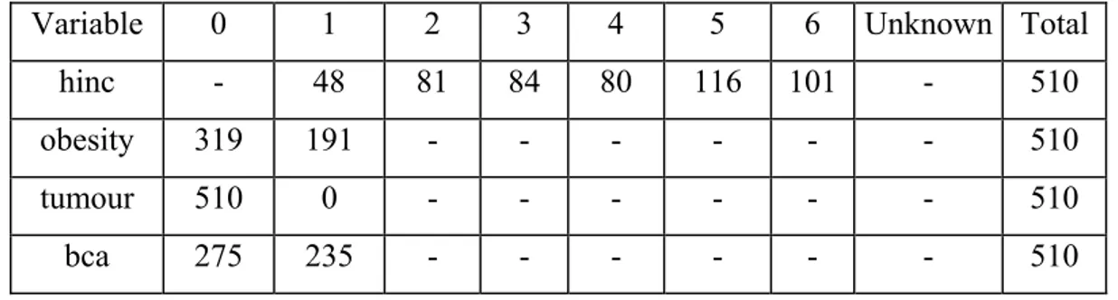
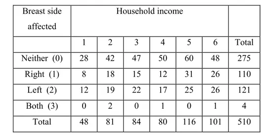
7.3 Analysis of the breast cancer data ... 71
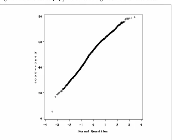
7.3.1 Descriptive analysis... 71
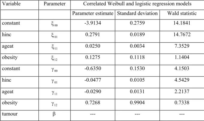
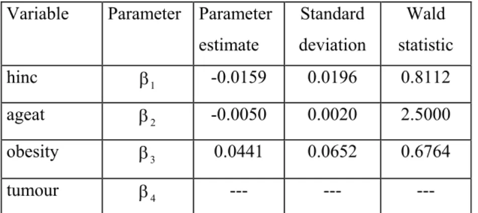
7.3.2 Model for the second level nesting ... 72
8 Discussion ... 76
APPENDIX ... 78
Appendix A: Symbols... 78
Appendix B: Definitions ... 80
Appendix C: Newton-Raphson method ... 82
Appendix D: Mathematical addendum ... 83
Appendix E: Tables... 97
Appendix F: Figures ... 100
References ... 105
ACKNOWLEDGEMENTS
I would like to thank my supervisors, Prof. Wolfgang Urfer and PD Dr. Jürgen Groß, for their guidance and inspiration throughout my research. I would also like to thank my external supervisor, Prof. George E. Bonney, for encouraging me to work on the topic of my thesis and for permitting me to use the oesophageal cancer data and the breast cancer data.
My thanks go to the “Studentensekretariat” of the University of Dortmund for offering me a scholarship to pursue this research.
Special thanks go to my mother, Victoria Vanderpuije, and to my sisters, Paulina Odai and Patience Odai, for their encouragement. I am indebted to Dr. Kepher Makambi, Dr. John Kwagyan and Mr. Joachim Kötting for their helpful suggestions which improved my work. I am also indebted to Messrs. Patrice Wandja, Hayford-Seth Badu, Kayode Adekeye, Jürgen Schweiger, Joachim Gerß, Ralf Offele, to Mesdames Anja Wollsiefen, Bärbel Skopp, Brigitte Koths, Isabelle Grimmenstein, Lisete Sousa, Magdalena Thöne, to Doctors K.-H. Loesgen, J.
Elsner, M. Brunnert, S. Selinsky, P. Hahnen, and to Professors H. Schulte and J. Hartung for their help and inspiration.
Finally, I would like to thank all friends and well-wishers for various forms of support they gave me during my studies.
1 Background and literature review
1.1 Introduction
The outcomes of family members are correlated because they share common risks. Thus standard methods of epidemiology, which assume independence of outcomes, are unsuitable for the analysis of family data. The disposition model is one of the possible models for the analysis of correlated binary data. It enables the characterisation of the dependence structure of a family and the response probabilities associated with it. The development of the disposition model involves the derivation and parameterisation of the joint distribution on which the likelihood function is based. Here, the experimental unit is the nuclear family and the response is the disease status. In such studies, the methods of estimating the parameters of the models are of particular importance. Here, the maximum likelihood method will be used to analyse the models. Since closed-form solutions are not possible, the Newton-Raphson iteration method is applied to obtain maximum likelihood estimates of the parameter vector. It should however be pointed out that maximum-likelihood becomes increasingly intractable as the model becomes more complex. Despite this limitation, the maximum likelihood is widely used, because it can provide accurate estimates and has some attractive optimum properties, such as asymptotically normally distributed estimators and best asymptotically normal sequence of estimators (Mood et al., 1974). Also, the maximum likelihood estimators possess the quality of functional invariance: if λ$ is the maximum likelihood estimator for λ, then
h(λ$) will be the maximum likelihood estimator of h( )λ for any function h(.) (Stuart, Ord and Arnold, 1999). In this way, the maximum likelihood estimators for a wide variety of parameterisations can be determined. With this study, potential risk factors for a disease such as smoking, age and alcohol use can be examined. Also, it can be assessed whether the disease tends to aggregate in families as a result of common shared risks. Such knowledge is decisive for counselling in the aetiology of familial disease.
The rest of the thesis is organised as follows: Section 1.2 briefly reviews the correlated regression models. Section 1.3 explains why the disposition model of the Weibull-type regression can provide more reasonable solutions than that of the logistic-type regression. In
briefly reviews Cox’s regression model (Cox, 1972) for the analysis of failure data when explanatory variables are available. In Chapter 4, the disposition model (Bonney, 1998) and its associated likelihood function will be introduced. The first and second level extensions of the disposition model will be considered in Chapter 5. Inference for the models will be treated in the first three sections of Chapter 6. To estimate the parameters in the model, the joint function of all the clusters is required. However, there is no loss of generality if the joint function of a cluster is considered. Section 6.4 discusses the properties of the score function.
The likelihood ratio test and the Wald’s test will be introduced in Section 6.5 to test for the independence of familial aggregation of a disease. Section 6.6 is devoted to the comparison of the model fit of models. Chapter 7 is divided into three sections. The first, Section 7.1, contains the descriptions of two data sets: oesophageal cancer data and breast cancer data.
Section 7.2 illustrates the methods with the oesophageal cancer data. The application to the breast cancer data is presented in Section 7.3. Chapter 8 gives a summary of the work and discusses experiences gained.
1.2 Review of correlated regression models
In models for clustered binary data, measures of association are of primary interest when a particular pattern of infection is suspected in a family. In the search for an appropriate model for inference on response probabilities and correlations, the equations for the estimation of the parameters become more complex. Thus, the estimation of all parameters becomes more difficult as the cluster size gets larger.
Cox (1972) reviewed several methods that had been proposed for the analysis of multivariate binary data and outlined some new proposals. He suggested the use of logistic representations, in which the joint response probability is a quadratic exponential form, as the simplest, most flexible, and in many ways the most important models. In the paper ‘Partial likelihood’, Cox (1975) gave a definition of partial likelihood which generalises the ideas of conditional and marginal likelihood. Here, he transformed the random variable Y into a sequence {X Sj, }j , j = 1,...,m, and decomposed the full likelihood of the sequence into two products, the second product being the partial likelihood based on S in the sequence {X Sj, }j . He pointed out that the partial likelihood is especially useful when it is appreciably simpler than the full likelihood. This is the situation when constructive procedures for finding useful partial likelihoods are provided, so that the partial likelihood involves only the parameters of interest and not nuisance parameters. To support this point, he made mention of the failure of the method of maximum likelihood as a general technique, especially in the sampling theory and pure likelihood approaches, due to excessive nuisance parameters, and hence the need to reduce dimensions. Care should however be taken to ensure that all or nearly all the relevant information is contained in the partial likelihood.
Liang and Zeger (1986) introduced the use of ‘generalised estimating equations’ (GEE), an extension of generalised linear models, for estimating regression parameters in situations when the vector of association parameters is a nuisance parameter. The approach is to use a working generalised linear model for the marginal distribution of the outcome variable. The method gives efficient estimates of regression coefficients, although estimates of the association among the binary outcomes can be inefficient. Liang, Zeger and Qaqish (1992)
analysis of multivariate binary data, focusing on the regression and association parameters.
They recommended the use of GEE1, introduced by Liang and Zeger (1986), when the association parameter is considered as a nuisance and the number of clusters is large relative to the size of each cluster. On the other hand, GEE2, introduced by Zhao and Prentice (1990), is preferable to GEE1 when there are few clusters and/or the association parameter is of primary interest. Connolly and Liang (1988) introduced the conditional logistic regression models for correlated binary data which are most useful when the dependence among observations is of main interest (such as in family data). Although the estimating functions are easily computed and have high efficiency compared to the computationally intensive maximum likelihood approach, more work is needed to determine the form of the weights used for the estimating functions U( , )β θ . Prentice (1988) considered regression methods for the analysis of correlated binary data when each binary observation may have its own covariates. In the case of the stratified and mixture models, he generalised the binary logistic regression model for the response Yi given the covariate xi to blocked binary data by setting
( )
) x exp(
1
] Y ) x exp[(
x ,i , Y
| Y Pr
i s
i i s i
s + α + β
β +
= α l≠
l , where αs is a parameter for the sth block. In the case of the conditional models, he specified a distribution (e.g., the logistic regression model) for each binary variate given all of the other variates in the block. Here, unlike the stratified and mixture models, one may allow the logistic location parameter to depend on the other binary responses in the same block.
Zhao and Prentice (1990) reparameterised probability distribution of the model advocated by Cox (1972) in terms of marginal parameters of ready interpretation. Since this approach yields models with very complicated marginal response probabilities and pairwise correlations, they suggested the transformations of the canonical parameters ( ,θ λk k), k = 1,...,K, to response means (µk =µ βk( ) ) and covariances (σk =σ β αk( , ) ), where β and α are parameter vectors. Scoring estimating functions can then be used to evaluate mean and correlation parameters under the quadratic exponential family. Qaqish and Liang (1992) presented a model for correlated binary data, in which the marginal expectation of each binary variable and the association between pairs of outcomes are modelled separately in terms of explanatory variables. With examples, they described some drawbacks of conditional models,
especially in situations where observations are missing or cluster sizes differ. On the other hand, the marginal model is reproducible, since the marginal distribution of any proper subset ( ,...,Y1 Yn) is of the same form. Hence the situation where a subset of the cluster ( ,...,Y1 Yn) is missing causes no problem. Carey, Zeger and Diggle (1993) proposed the use of odds ratios to measure association among responses. The approach, which alternates between two steps, estimates the association parameters by modelling the conditional distribution of one response given another. The alternating logistic regression avoids the computational burdens encountered in many problems, and its estimates are reasonably efficient relative to solutions of second-order methods.
In order to accommodate the many complicating features associated with real data, Bonney (1998) derived joint distributions for constructing likelihood functions. The central aspects of his work concern the notion of disposition to an outcome. He used a moment series representation to derive the joint distributions. Kötting, Bonney and Urfer (1998) used the ordinal-disposition-transitional model, an extension of the disposition model, to analyse dynamic changes of damage in forest-ecosystems. Odai et al. (2002) discussed the use of the correlated Weibull regression model for the analysis of multivariate binary data. The results have shown that the model provides feasible means of analysing family data.
In this dissertation, computationally attractive models with readily interpretable dependence structure for the regression analysis of correlated binary data will be presented. Estimation is based on the log-likelihood function, whose solutions can be solved by the Newton-Raphson iteration. The implications of higher level nesting in relation to the dimension of the parameter space will also be examined.
1.3 Motivation
Logistic regression is by far the most common approach to modelling the relationship between some explanatory variables and a binary response variable. This approach sometimes leads to biased estimates of covariate effects since it does not take care of dependence of outcomes. In order to incorporate dependence within families into regression models, Bonney (1998) developed the disposition models for the analysis of family data. He considered the logistic-type regression (Bonney, 1998) as the basic regression function in the non-nested disposition model. However, there are situations in which the response of interest is not a binary risk, but rather the time to failure. This is especially the case if one, for instance, wishes to know if a particular disease occurs at a certain point in time or at a certain age. The standard Weibull distribution is also inadequate for the analysis of family data, because it is not equipped with a dependence structure to take care of correlated outcomes. Furthermore, explanatory variables cannot be included in the statistical analysis. It will therefore be appropriate to consider the Weibull-type regression (Bonney, 1998) as the basic regression function in Bonney’s disposition model (Bonney, 1998). Thus, in general, the correlated Weibull regresion model distinguishes itself from the correlated logistic regression model in the sense that it takes into account the special features of the underlying data (e.g., it is more suitable for the analysis of data drawn from failure distributions).
2 The standard Weibull distribution
The purpose of this section is to review some basic concepts of survival theory of the standard Weibull distribution. This is necessary since there is a link between the constructions of the likelihood functions of the standard Weibull distribution and the correlated Weibull regression model. This link will be discussed at the end of Chapter 4.
Consider the two-parameter Weibull distribution denoted by T~ W(φ,ρ) (φ>0,ρ>0), where T is the lifetime of a living organism or a product, or the time until the occurrence of some specified event, φ is the shape parameter and ρ is the scale parameter, and let
n 2 1,T ,...,T
T be a random sample of size n from T.
The probability density function (PDF), which is sometimes also called the unconditional failure rate, is given by
φρ −ρ >
= ρ
φ φ− φ
otherwise
0,
0 t ), t exp(
) t ,
; t ( f
1
T , (2.1)
where φ > 0, ρ > 0 are real parameters (Gross and Clark, 1975).
The cumulative distribution function (CDF)
>
ρ
−
−
= ≤
≤
= ρ
φ φ
0 t ), t exp(
1
0 t ) 0,
t T ( P ) ,
; t (
FT (2.2)
is called the lifetime distribution or failure distribution. If T represents time at death of an individual, FT(t;φ,ρ) is the probability that an individual dies before time t. On the other hand, if T represents age of first occurrence of a certain event (e.g., chronic disease), then
) ,
; t (
FT φ ρ represents age of onset distribution of the event (disease) (Gross and Clark, 1975;
Elandt-Johnson and Johnson, 1980).
The survival function (SF), which is defined as the probability of an individual surviving beyond time t, is given by
ST(t)=Pr(T>t)=1−FT(t;φ,ρ)=exp(−ρtφ) (2.3)
(Gross and Clark, 1975; Elandt-Johnson and Johnson, 1980). In survival analysis, ST(t) is more commonly used, instead of its complementary function, FT(t;φ,ρ).
The hazard function (HF), which characterises the instantaneous failure rate when T = t, conditional on survival to time t, is defined mathematically as
∆
>
∆ +
<
= <
→
∆ t
) t T
| t t T t lim Pr(
) t (
hT t 0 (2.4)
(Gross and Clark, 1975). The hazard function, also termed the failure rate, may also be defined as a measure of proneness to failure. This can also be expressed as
e T 1
T T
T log S (t) t
dt d )
t ( S
) t ( dyS
d ) t (
h =− =− =φρ φ− (2.5)
(Gross and Clark, 1975; Nelson, 1972). For values of the shape parameter, φ, less than 1, the hazard function is a decreasing function, for φ = 1, the Weibull distribution is an exponential distribution and has a constant failure rate, and for φ > 1, it is an increasing function of t (Nelson, 1972). An increasing hazard rate indicates that a unit of age t is more likely to fail in a given increment of time than it would be in the same increment of time at an earlier age. For example, the probability that an individual survives to age 71, given that he has lived to age 70, is greater than the probability that an individual survives to age 72, given that he has lived to age 71. Similarly, a decreasing hazard rate means that the unit is improving with age. For example, children who have undergone an operative procedure to correct a congenital condition such as a heart defect represent a population exhibiting a decreasing hazard rate.
thereafter (Gross and Clark, 1975). A constant hazard rate results due to chance failures (e.g., accidents). Such random occurrences are often independent of age.
The failure rate function of a discrete distribution { }pk ∞k=0 (e.g., geometric, binomial, poisson, etc.) is
∑∞
=
=
k
j j
k
p ) p k (
h , (2.6)
where k is the number of failures (Barlow and Proschan, 1965). We note that in this case 1
) k (
h ≤ .
From (2.1), (2.3) and (2.5), it follows that
fT(t)=hT(t)ST(t). (2.7)
Any distribution of survival times can be characterised by the three equivalent functions )
t (
fT , hT(t) and ST(t).
In observational studies of the time to failure of units (e.g., breakdown of a machine, death of an individual), a group of data may be incomplete in the sense that some units may not have failed by the end of the study, or may have been withdrawn before the end of the study. Such data are said to be censored (Daintith and Nelson, 1989).
Censoring is said to be on the right when the item or subject is observed prior to failure or death. Since the event time is larger than the time of observation, such an observation provides information on the survival function, ST(t), evaluated at the time of observation (Klein and Moeschberger, 1997).
On the other hand, censoring is said to be on the left when failure or death occurs prior to some designated censoring time. Since the event time has already occurred, such an
observation provides information on the cumulative distribution function, FT(t), evaluated at the time of observation (Klein and Moeschberger, 1997).
An observation corresponding to an exact event time provides information on the density function of T, fT(t), at this time (Klein and Moeschberger, 1997).
The likelihood function may take the following form:
∏ ∏ ∏
∈ ∈
∈
∝
R
j j L
j T j T D
j
j
T(t ) S (t ) F (t )
f
L , (2.8)
where, D is the set of death times, R the set of right-censored observations and L is the set of left-censored observations (Klein and Moeschberger, 1997). If the data set comprises only right-censored and left-censored observations, the above likelihood function reduces to
∏ ∏
∈ ∈
∝
R
j j L
j T j
T(t ) F (t )
S
L . (2.9)
The following are some examples on censored data.
Ex. 1: In a particular clinical trial, suppose that all n patients are followed until death. Their recorded survival times are t1,...,tn, and it is assumed that the death density function for the jth patient is given by the Weibull density function. The likelihood function L(t;φ,ρ) is given by
∏ ∏
=
φ
− φ
=
ρ
− φρ
= ρ φ
= ρ
φ n
1 j
j 1
j n
1 j
j; , ) t exp( t )
t ( f ) ,
; t (
L (2.10)
(Gross and Clark, 1975).
Ex. 2: Suppose that we only know that out of n individuals starting at time zero, r died before time 't, and (n – r) survived beyond 't (i.e., censored data). The statistical model for this set of data is binomial, so that the likelihood function is
[FT(t;' )]r[ST(t;' )]n r r
) n ,
; t (
L θ θ −
= ρ
φ (2.11)
(Elandt-Johnson and Johnson, 1980).
3 Cox’s regression model
The Cox model (also known as the proportional hazards model) is a model that can be used for the analysis of failure data when explanatory variables are available. There will be a brief review of this model and its estimation procedure in this chapter.
3.1 The model
Let )h(t;x be the hazard rate at time t for an individual with risk vector xT =(x1,...,xp). Cox (1972) specified his model as follows:
h(t;x)=h0(t)exp(βTx), (3.1.1)
where )h0(t is an arbitrary baseline hazard rate and βT =(β1,...,βp) is a vector of unknown parameters.
The above model is often called a proportional hazards model because, the ratio of the hazard rates of two individuals with covariate values x and x can be expressed as '
β −
= ∑
= p
1 k
' k k
k(x x )
) exp ' x
; t ( h
) x
; t (
h , (3.1.2)
which is a constant (see, for example, Klein and Moeschberger, 1997). This indicates that the hazard rates are proportional. The quantity (3.1.2), called the relative risk (hazard ratio), gives the factor by which the risk of an individual with covariate x is increased in comparison to an individual with risk factor 'x .
3.2 Parameter estimation
In order to estimate the parameters in Cox’s model with the maximum likelihood method, the baseline hazard, h0(t), must be specified. To deal with this situation, Cox exploited the definition of partial likelihood. Specifically, he considered the baseline hazard, h0(t), as a nuisance parameter function and concentrated mainly on the regression parameters.
Let t(1) <t(2) <...<t(n) denote the ordered event times and define the risk set at time t , (i) )
t (
R (i) , ni=1,..., , as the set of all individuals who are still under study at a time just prior to
) i
t . Further, let ( x denote the value of x for the jth individual, and j x the value for the (i) individual failing at time t , (i) i=1,...,n. Then, Cox (1972) gave the partial likelihood based on the hazard function specified by (3.1.1) as
∏ ∑=
∈
β
= β
β n
1 i
) t ( R j
j T
) i ( T
) i (
) x exp(
) x ) exp(
(
L . (3.2.1)
It should be noted that the numerator of the likelihood in (3.2.1) depends only on information
about all individuals who have not yet experienced the event (Klein and Moeschberger, 1997).
Direct calculation from the log-likelihood gives the score equation
∑ ∑ ∑∑
= =
∈
∈
β β
−
=
β n
1 i
n
1 i
) t ( R j
j T )
t ( R j
j T j
) i (
) i ( ) i (
) x exp(
) x exp(
x x
) (
U , (3.2.2)
from which we obtain the Hessian matrix
∑ ∑
∑
=
∈
∈
β β
− β β
=
β n
1 i
) t ( R
j j
T )
t ( R j
j T T
j j T
) i ( ) i (
) i ( ) i (
) x exp(
) x exp(
x x )
( A ) ( A ) (
H , (3.2.3)
where
∑
∑
∈
∈
β β
=
) t ( R j
j T ) t ( R j
j T j
) i (
) i ( ) i (
) x exp(
) x exp(
x
A , i=1,...,n.
The Fisher information matrix is given by
β β
β β β −
β
=
β ∑
∑ ∑∑ ∑
∑ ∑
∑
∈
∈
=
∈
∈
=
∈
∈
) t ( R j
j T )
t ( R j
j T T
n j
1 i
) t ( R j
j T ) t ( R j
j T n j
1 i
) t ( R j
j T )
t ( R j
j T T
j j
) i ( ) i (
) i ( ) i (
) i ( ) i (
) x exp(
) x exp(
x )
x exp(
) x exp(
x )
x exp(
) x exp(
x x )
(
I (3.2.4)
(Klein and Moeschberger, 1997). Cox (1975) has shown that the usual maximum likelihood properties hold for estimates and tests based on partial likelihoods.
4 Introduction of the non-nested disposition model
Disposition, as defined by Bonney, is the tendency of an individual or group to manifest an outcome (e.g., to be affected by a disease). The central aspect of the development of the disposition model is the derivation of joint distributions that directly capture aggregation, if there should be any. In this chapter, there will be a brief presentation of the disposition model (Bonney, 1998) and its associated joint distribution function.
Consider a binary outcome Y = 1 or 0, with q0 group-specific covariates, Z (Z ,...,Z )
q0
0 01 T
0 = ,
and p individual-specific covariates, XTj =(Xj1,...,Xjp), j=1,...,n, measured on several groups of individuals. We consider two types of dispositions here: the group disposition, δ0, which is determined by the group-specific covariates, Z0, and the individual disposition, δj, which is determined by the group-specific covariates, Z0, and the individual-specific covariates, X , j j=1,...,n.
Define the group or overall disposition, δ0, by
δ µ
0 α0
0
= , (4.1)
where µ0 is the baseline disposition under no aggregation and α0 is the relative disposition.
Then, α0 < 1 corresponds to positive aggregation, α0 = 1 corresponds to no aggregation, and α0 > 1 corresponds to negative aggregation.
The logit of the group disposition can be written as
δ
where
M Z0 0 0 1 0
( ) log=
− µ
µ (4.3)
and
D Z0 0 0
0
0
1 1 0
( ) log= log
− −
− δ
δ
µ
µ . (4.4)
We term M Z0( 0) the logit of group disposition assuming no aggregation or the cluster logit mean risk and D Z0( 0) the excess disposition due to aggregation or the excess cluster logit disposition due to dependence among members of a group.
From (4.3) and (4.4), it follows that
µ0
0 0
1
=1
+exp{ [− M Z( )]}, δ0
0 0 0 0
1
= 1
+exp{ [− M Z( )+D Z( )]} (4.5) and therefore
α µ δ
0 0
0
0 0 0 0
0 0
1
= = + 1 − +
+ −
exp{ [ ( ) ( )]}
exp{ [ ( )]}
M Z D Z
M Z . (4.6)
Now, we decompose the logit of the individual disposition as
M (Z ) D (Z ) W (X )
log1 0 0 0 0 j j
j
j = + +
δ
−
δ =: θj, (4.7)
j = 1,…,n, where M0(Z0) and D0(Z0) are as defined above, and W Xj( j) is a function of the individual-specific covariates. It follows that
)]}
X ( W ) Z ( D ) Z ( M [ exp{
1
1 )
exp(
1 1
j j 0 0 0 0 j
j = + − + +
θ
−
= +
δ , (4.8)
j = 1,…,n.
The joint probability for a group or cluster becomes
∏ ∏
=
−
=
δ
− δ α +
− α
−
=
=
= n
1 j
y 1 j y
j 0 n
1 j
j 0
n n 1 1
j
j(1 )
) y 1 ( ) 1 ( ) y Y ,..., y Y (
P , (4.9)
with α0 and δj as defined in (4.6) and (4.8). Explicit derivation of the joint distribution can be found in Bonney (1998). If α0 =1 or D0(Z0)=0, equation (4.9) reduces to
∏
=
δ −
− δ
=
=
= n
1 j
y 1 j y j n
n 1 1
j
j(1 )
) y Y ,..., y Y (
P , (4.10)
that is, the independence case. Explicit parameterisations for M Z0( 0) and D Z0( 0) are obtained by the linear models
M Z0 0 00 01Z01 0q Z0q
0 0
( )=ξ +ξ + +... ξ (4.11)
and
D Z0( 0)=γ00 +γ01Z01+ +... γ0q0Z0q0. (4.12)
The set of parameters to be determined in the model is
) ,..., , ,..., , ,..., ( ) , ,
(ξ0 γ0 β = ξ00 ξ0q0 γ00 γ0q0 β1 βp
=
λ .
It is now convenient to compare and contrast the standard Weibull distribution with the correlated Weibull regression model. We denote the likelihood function of the joint distribution in Equation (4.9) by Lk(λ|y), Kk=1,..., :
∏
∏ =
−
=
δ
− δ α +
− α
−
=
λ n
1 j
y 1 j y j 0 n
1 j
j 0
k
j
j(1 )
) y 1 ( ) 1 ( ) y
| (
L ,
1 exp{ [M (Z ) D (Z ) (1 exp( X ... X ))]}
1
jp p 1
j 1 0
0 0 0
j = + − + + − β + +β
δ , j = 1,…,n, and recall that
the likelihood function for the standard Weibull distribution based on (2.9) is
∏ ∏
∈ ∈
∝
R
j jL
j T j
T(t ) F (t )
S
L .
The following differences are observed. (1) In the case of the standard Weibull distribution, the response variable is a variable of time (continuous or discrete), whereas the response variable in Bonney’s disposition model presented in this dissertation is the disease status, and
therefore binary. (2) As opposed to the standard Weibull distribution whose most applied characterisation revolves around its role in extreme value theory (e.g., daily maximum or minimum temperatures, precipitation, etc.), Bonney’s model is fitted with parameters like δj and α0 to model the effect of influential factors and to capture aggregation in families, if there should be any. Here, variables of time (e.g., age) are regarded as covariates in the model. Our concern, however, is to determine the link between the standard Weibull distribution and the correlated Weibull regression model. Suppose T is the length of time until the occurrence of a certain disease, and consider a group of size n with survival times
n 1,...,T
T , where T is censored or not at time j t with the censoring indicator j yj =0 if censored, and yj =1 if uncensored. Then, in the above likelihood functions, yj =0 in the correlated Weibull regression model corresponds to the survival function in the standard Weibull distribution, and yj =1 in the correlated Weibull regression model corresponds to the cumulative distribution function in the standard Weibull distribution. In other words,
∏=
δ
− α
+ α
−
=
λ n
1 j
j 0
0
k( |y) (1 ) (1 )
L
∏
= + − + + − β + +β
β + + β
− + +
α − + α
−
= n
1
j 0 0 0 0 1 j1 p jp
jp p 1
j 1 0
0 0 0 0
0 1 exp{ [M (Z ) D (Z ) (1 exp( X ... X ))]}
))]}
X ...
X exp(
1 ( ) Z ( D ) Z ( M [ ) exp{
1 (
corresponds to ∏
∈
∝
R j
j T(t ) S
L = ∏
∈
ρ φ
−
R j
j ) t exp( , and
∏= + − + + − β + +β α
=
λ n
1
j 0 0 0 0 1 j1 p jp
0
k 1 exp{ [M (Z ) D (Z ) (1 exp( X ... X ))]}
) 1 y
| ( L
corresponds to ∏ ∏
∈
φ
∈
ρ
−
−
=
∝
L j
j L
j
j
T(t ) {1 exp( t )}
F
L , with the above parameters as previously
defined. Thus, in this sense, the two likelihood functions are equivalent.