Adaptive Estimation of Time Varying Copulae

(1)

Adaptive Estimation of Time Varying Copulae

Master Thesis submitted to

Prof. Dr. Wolfgang Härdle Prof. Dr. Vladimir Spokoiny

Institute for Statistics and Econometrics

CASE - Center for Applied Statistics and Economics

Humboldt-Universität zu Berlin

by

Ekaterina Ignatieva (184944)

in partial fulfillment of the requirements

for the degree of Master of Sciences in Statistics

Berlin, September 6, 2005

(2)

Declaration of Authorship

I hereby confirm that I have authored this master thesis independently and without use of others than the indicated sources. All passages which are literally or in general matter taken out of publications or other sources are marked as such.

Berlin, September 6, 2005

Ekaterina Ignatieva

(3)

List of Figures

4.1 Density of a Gaussian copula with ρ= 0.5. . . 23

4.2 Density function of F(x₁, x₂) with ρ= 0. . . 23

4.3 Contour plot of the Gaussian copula, ρ= 0. . . 24

4.4 Density of a Gumbel-Hougaard copula with θ= 2.5. . . 25

4.5 Density of a Clayton copula with θ = 1.5 . . . 26

4.6 Contour plots of the Gumbel-Hougaard and Clayton copulae, θ = 1.5 26 4.7 10000-sample output with fixed σ₁ = 1, σ₂ = 1 of the Gumbel- Hougaard and Clayton copulae, θ = 1.5 . . . 27

4.8 Density of a AMH copula with θ = 0.8 . . . 28

4.9 Density of a Frank copula with θ = 5.0 . . . 28

4.10 Contour plots of the AMH copula withθ = 0.8and Frank copula with θ = 5.0 . . . 29

4.11 10000-sample output with fixed σ₁ = 1, σ₂ = 1 of the AMH copula, θ = 0.8 and Frank copula, θ = 5.0 . . . 29

6.1 Dax and Dow Jones log-returns for the period January 1, 1997 to March 20, 2004 (1573 observations). . . 36

6.2 Density of the Dax log-returns (red) and normal density (black), estimated nonparametrically using Quartic kernel with bh= 1.06bσn⁻¹⁵ . 37 6.3 Density of the Dow Jones log-returns (blue) and normal density (black), estimated nonparametrically using Quartic kernel with bh= 1.06bσn⁻¹⁵ . 37 6.4 Parameters δˆ₁ and δˆ₂ estimated from normal marginals of the Dax and Dow Jones log-returns (upper respectively middle panel) and estimated copula dependence parameter θˆ(lower panel). The resultes are obtained using IFM method with moving time window n= 250. . 39

6.5 Dax and Dow Jones log-returns at minimal dependence (November 30, 2000). . . 40

6.6 Dax and Dow Jones log-returns at maximal dependence (March 11, 2004). . . 40

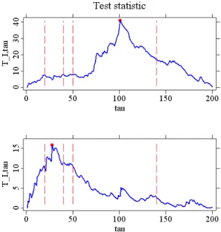
7.1 Test statistics TI,τ for one fixed intervalI plotted against τ. Jump at the middle point (τ = 100) and not at the middle point (τ = 30) are represented by the upper and lower panel, respectively. . . 44

(6)

List of Figures

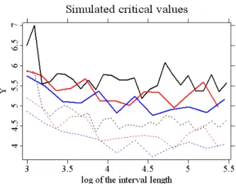
8.1 One simulation of the copula parameter θ: real (red) and estimated (blue). The results are obtained with parametersα = 0.05,m₀ = 20, c= 1.1, ρ₁ = 0.1, ρ₂ = 0.3 . . . 46 8.2 Critical values for α = 0.05 (solid line) and α = 0.1 (dashed line),

computed by simulations using Gumbel-Hougaard copula with parameters m₀ = 20, ρ₂ = 0.3 and c = 1.1, ρ₁ = 0.1 (black line), c= 1.2, ρ₁ = 0.2(red line), c= 1.25,ρ₁ = 0.25(blue line). . . 47 8.3 Pointwise mean (blue line) based on 200 simulations of the data,

simulated from the Gumbel-Hougaard copula and real parameter (dashed lines). The left panel represents a jump size equal to 2, the right panel represents a jump size equal to 1. The results are obtained with parameters m₀ = 20, ρ₂ = 0.3 and c = 1.1, ρ₁ = 0.1 (upper panel); c = 1.2, ρ₁ = 0.2 (middle panel); c= 1.25, ρ₁ = 0.25 (lower panel). . . 48 8.4 Pointwise median (red line) and quartiles (dashed lines) for the es-

timates of the copula parameter θ_t, based on 200 simulations of the data, simulated from the Gumbel-Hougaard copula. The left panel represents a jump size equal to 2, the right panel represents a jump size equal to 1. The results are obtained with parameters m₀ = 20, ρ₂ = 0.3andc= 1.1,ρ₁ = 0.1(upper panel);c= 1.2,ρ₁ = 0.2(middle panel); c= 1.25, ρ₁ = 0.25 (lower panel). . . 49 8.5 Critical values for α = 0.05 (solid line) and α = 0.1 (dashed line),

computed by simulations using Clayton copula with parameters m₀ = 20,ρ₂ = 0.3 andc= 1.1, ρ₁ = 0.1 (black line), c= 1.2, ρ₁ = 0.2 (red line), c= 1.25,ρ₁ = 0.25(blue line). . . 55 8.6 Pointwise mean (blue line) based on 200 simulations of the data,

simulated from the Clayton copula and real parameter (dashed line).

The left panel represents a jump size equal to 2, the right panel represents a jump size equal to 1. The results are obtained with parameters m₀ = 20, ρ₂ = 0.3 and c= 1.1, ρ₁ = 0.1 (upper panel);

c= 1.2, ρ1 = 0.2 (middle panel); c= 1.25, ρ1 = 0.25 (lower panel). . . 56 8.7 Pointwise median (red line) and quartiles (dashed lines) for the es-

timates of the copula parameter θ_t, based on 200 simulations of the data, simulated from the Clayton copula. The left panel represents a jump size equal to 2, the right panel represents a jump size equal to 1. The results are obtained with parameters m₀ = 20, ρ₂ = 0.3 and c= 1.1,ρ1 = 0.1(upper panel); c= 1.2, ρ1 = 0.2 (middle panel);

c= 1.25,ρ₁ = 0.25(lower panel). . . 57 8.8 Kullback-Leibler information number K(θ₁, θ₂) (upper panel) and

K(θ2, θ1) (lower panel) plotted againstθ2 for fixed θ1 = 1. The blue line refers to the Gumbel-Hougaard copula and the red line to the Clayton copula. . . 58

(7)

List of Figures

9.1 Marginal parameters for DaimlerChrysler (upper panel) and Volkswa- gen (lower panel) estimated by exponential smoothing with parameter λ= 1/20. . . 61 9.2 Stock price process (upper panel), log returns (middle panel) and

copula dependence parameter θ (lower panel) for DaimlerChrysler (black line) and Volkswagen (red line). The estimates ofθare obtained with parametersm₀ = 20, c= 1.25, ρ₁ = 0.25, ρ₂ = 0.3 and α= 0.05. 62 9.3 Upper panel: estimated copula dependence parameter θ for Daimler-

Chrysler and Volkswagen (blue line) and its mean (red line). Lower panel: estimated intervals of time homogeneity. The results are obtained with parameters m₀ = 20, c = 1.25, ρ₁ = 0.25, ρ₂ = 0.3 and α = 0.05. . . 63 9.4 Marginal parameters for Allianz (upper panel) and Münchener Rück-

versicherung (lower panel) estimated by exponential smoothing with parameter λ= 1/20. . . 64 9.5 Stock price process (upper panel), log returns (middle panel) and

copula dependence parameter θ (lower panel) for Allianz (black line) and Münchener Rückversicherung (red line). The estimates of θ are obtained with parameters m₀ = 20, c= 1.25, ρ₁ = 0.25, ρ₂ = 0.3 and α = 0.05. . . 65 9.6 Upper panel: estimated copula dependence parameter θ for Allianz

and Münchener Rückversicherung (blue line) and its mean (red line).

Lower panel: estimated intervals of time homogeneity. The results are obtained with parameters m₀ = 20, c= 1.25, ρ₁ = 0.25, ρ₂ = 0.3 and α = 0.05. . . 66 9.7 Marginal parameters for Bayer (upper panel) and BASF (lower panel)

estimated by exponential smoothing with parameter λ= 1/20. . . 67 9.8 Stock price process (upper panel), log returns (middle panel) and

copula dependence parameter θ (lower panel) for Bayer (black line) and BASF (red line). The estimates ofθ are obtained with parameters m0 = 20, c= 1.25, ρ1 = 0.25,ρ2 = 0.3 and α= 0.05. . . 68 9.9 Upper panel: estimated copula dependence parameterθ for Bayer and

BASF (blue line) and its mean (red line). Lower panel: estimated intervals of time homogeneity. The results are obtained with parameters m₀ = 20, c= 1.25, ρ₁ = 0.25,ρ₂ = 0.3 and α= 0.05. . . 69 9.10 Upper panel: estimated copula dependence parameterθfor 4-dim data:

DaimlerChrysler, Volkswagen, Bayer and BASF (blue line) and its mean (red line). Lower panel: estimated intervals of time homogeneity.

The results are obtained with parametersm₀ = 20,c= 1.25,ρ₁ = 0.25, ρ2 = 0.3and α = 0.05. . . 70

(8)

List of Figures

9.11 Upper panel: estimated copula dependence parameterθfor 6-dim data:

DaimlerChrysler, Volkswagen, Bayer, BASF, Allianz and Münchener Rückversicherung (blue line) and its mean (red line). Lower panel:

estimated intervals of time homogeneity. The results are obtained with parametersm₀ = 20, c= 1.25, ρ₁ = 0.25, ρ₂ = 0.3 and α= 0.05. 71

(9)

List of Tables

6.1 Descriptive statistics for δˆ₁, δˆ₂,θˆ. . . 38 8.1 Descriptive statistics for the detection speeds to sudden jumps of the

Gumbel-Hougaard copula dependence parameter with a jump size of 2. The results are obtained with parameters α = 0.05, m₀ = 20, ρ2 = 0.3 and different parameters c and ρ1. Statistics are based on 200 simulations. . . 50 8.2 Descriptive statistics for the detection speeds to sudden jumps of the

Gumbel-Hougaard copula dependence parameter with a jump size of 1. The results are obtained with parameters α = 0.05, m₀ = 20, ρ₂ = 0.3 and different parameters c and ρ₁. Statistics are based on 200 simulations. . . 51 8.3 Descriptive statistics for the detection speeds to sudden jumps of the

Clayton copula dependence parameter with a jump size of 2. The results are obtained with parameters α = 0.05,m₀ = 20, ρ₂ = 0.3and different parameters c and ρ₁. Statistics are based on 200 simulations. 53 8.4 Descriptive statistics for the detection speeds to sudden jumps of the

Clayton copula dependence parameter with a jump size of 1. The results are obtained with parameters α = 0.05,m₀ = 20, ρ₂ = 0.3and different parameters c and ρ₁. Statistics are based on 200 simulations. 54 8.5 Kullback-Leibler information number K(θ₁, θ₂)andK(θ₂, θ₁)for fixed

θ₁ = 1and parameter θ₂ = 2.0,3.0; for the Gumbel-Hougaard and the Clayton copula. . . 55

(10)

1 Introduction

“...as well as being one of the most ubiquitous concepts in modern finance and insurance, correlation is also one of the most misunderstood concepts. Some of the confusion may arise from the literary use of the word to cover any notion of dependence. To a mathematician correlation is only one particular measure of stochastic dependence among many. It is the canonical measure in the world of multivariate normal distribution functions, and more generally for spherical and elliptical distributions. However, empirical research in finance and insurance shows that the distributions of the real world are seldom in this class.”

Embrechts, Mc Neil and Straumann, 1999 In this chapter we will consider a concept of dependence. As we already know, the cumulative distribution function (cdf) of a 2-dimensional vector(X₁, X₂)is given by F(x1, x2) = P(X1 ≤x1, Y1 ≤y1) (1.1) For the case that X₁ and X₂ are independent, their joint cumulative distribution functionF(x₁, x₂) can be written as a product of their 1-dimensional marginals:

F(x1, x2) = FX1(x1)FX2(x2) =P (X1 ≤x1)P (X2 ≤x2) (1.2) But how can we representF(x₁, x₂)without having an information concerning the dependence of X₁ and X₂? How can we model the relationship between them?

Most people would model this by means of linear correlation. Several authors (e.g.

Embrechts, Mc Neil and Straumann, 1999) show therefore that the correlation is an appropriate measure of dependence only when the random variables have an eliptical or spherical distribution, which include the normal multivariate distribution.

Although the terms “correlation” and “dependency” are often used interchangeably, correlation is actually a rather imperfect measure of dependency, and there are many circumstances where correlation should not be used. We therefore need an alternative dependency measure that is reliable when correlation is not - and the answer is to use copulae.

Copulae represent an elegant concept of connecting marginals with joint cummulative distribution functions. Copulae are functions that join or “couple” multivariate

(11)

1 Introduction

distribution functions to their 1-dimensional marginal distribution functions. Let us consider a d-dimensional vector X = (X₁, ..., X_d). Using copulae, the marginal distribution functions F_X_i(i= 1, ..., d) can be separately modelled from their dependence structure and then coupled together to form the multivariate distributionF_X. Copula functions have a long history in probability theory and statistics since they date back to (Sklar, 1959). Their application in finance is very recent: the idea first appears in (Embrechts, Mc Neil and Straumann, 1999) in connection with correlation as a measure of dependence. Copulae constitute an essential part in quantitative finance (Härdle, Kleinow and Stahl, 2002) and are recognized as an important tool in Value-at-Risk (VaR) calculations. VaR is a measure that characterizes the riskiness of a portfolio; it keeps the probability of a negative outcome (portfolio losses) below some level λ.

DEFINITION 1.1. For a financial position X, we define its VaR at level λ as V aR_λ(X) = inf{m|P[X+m <0]≤λ} (1.3) In other terms, VaR is a quantile at level λ of the distribution of X:

V aR_λ(X) =F_λ⁻¹(X) (1.4)

To be able to model the VaR of a portfolio, we have to know as well the distribution of losses associated with the risk factors as a dependence structure within the portfolio. Formerly, there were two main approaches for modelling dependence structure: multivariate normality or independence. In both cases, risk aggregation is straightforward but often too far away from realistic models, since risk factors are seldom independent and can even have a dependence structure. To overcome this problem, we separate the study of the univariate behaviour of each variable from the study of dependence structure. The dependence structure of the random variables is known as acopula. The combination of a copula with specific univariate distributions then allows to construct a multivariate distribution, so-called copula-based models, which allow to calculate VaR more efficiently.

In this study we perform the copulae estimations using adaptive and non-adaptive techniques. This thesis can be seen as a preliminary study to risk management with adaptive copulae because it is the accurate basis for VaR calculations.

The thesis is organized as follows: chapter 1 and 2 are devoted to the introduction of basic definitions, and later to the definition and basic properties of a copula. Chapter 2 refers to the modelling dependence with copulae. Some examples of bivariate copulae and their extension to the multivariate case are represented in chapter 4 and chapter 5, respectively. Chapter 6 and 7 are devoted to the time-varying copulae.

(12)

1 Introduction

Full maximum likelihood (FML) estimation andInference for margins (IFM) methods are performed in the 6th chapter. Adaptive copula estimation, based onLocal change point analysis(LCPD) (Mercurio, Spokoiny, 2004) is represented in chapter 7. The change point test on the copula dependence parameterθ can improve substantially the dependence modelling. We illustrate the method considering some simulated examples (chapter 8) and then apply it to the 2-, 4- and 6-dimensional data sets from the Dax Index.

First let us concentrate on the 2-dimensional case, then we will extend this concept to the d-dimensional case, for a random variable in R^d with d≥1.

To be able to define a copula function, first we need to represent a concept of the volume of a rectangle, a 2-increading function and a grounded function.

Let U₁ and U₂ be two sets in R = R∪ {+∞} ∪ {−∞} and consider the function F :U₁×U₂ −→R.

DEFINITION 1.2. The F-volume of a rectangle B = [x₁, x₂]×[y₁, y₂]⊂U₁×U₂ is defined as:

VF(B) = F(x2, y2)−F(x1, y2)−F(x2, y1) +F(x1, y1) (1.5) DEFINITION 1.3. F is said to be a 2-increasing function if for every B = [x₁, x₂]×[y₁, y₂]⊂U₁×U₂,

V_F(B) ≥ 0 (1.6)

REMARK 1.1. Note, that “to be 2-increasing function” neither implies nor is implied by “to be increasing in each argument”.

The following lemmas (Nelsen, 1999) will be very useful later for establishing the continuity of copulae.

LEMMA 1.1. Let U₁ and U₂ be nonempty sets in R and let F :U₁×U₂ −→R be a two-increasing function. Let x1, x2 be in U1 with x1 ≤x2, andy1, y2 be in U2 with y₁ ≤ y₂. Then the function t 7→F(t, y₂)−F(t, y₁) is nondecreasing on U₁ and the function t7→F(x₂, t)−F(x₁, t) is nondecreasing on U₂.

DEFINITION 1.4. If U₁ and U₂ have a smallest element minU₁ and minU₂ respectively, then we say, that a function F :U₁×U₂ −→R is grounded if :

for all x∈U₁ : F(x,minU₂) = 0 and (1.7) for all y∈U₂ : F(minU₁, y) = 0 (1.8) In the following, we will refer to this definition of a distribution function :

(13)

1 Introduction

DEFINITION 1.5. A distribution function is a function from R

2 7→[0,1] which:

• is grounded

• is 2-increasing

• satisfies F (∞,∞) = 1

LEMMA 1.2. Let U₁ and U₂ be nonempty sets in R and let F :U₁×U₂ −→R be a grounded two-increasing function. Then F is nondecreasing in each argument.

Proof:

Set x₁ = minU₁ and y₁ = minU₂ in Lemma 1.1.

DEFINITION 1.6. If U₁ and U₂ have a greatest element maxU₁ and maxU₂ respectively, then we say, that a functionF : U₁×U₂ −→R has margins and that the margins of F are given by:

F(x) =F(x,maxU₂) for all x∈U₁ (1.9) F(y) =F(maxU1, y) for all y∈U2 (1.10) LEMMA 1.3. Let U₁ and U₂ be nonempty sets in R and let F : U₁ ×U₂ −→R be a grounded two-increasing function which has margins. Let (x₁, y₁), (x₂, y₂) ∈ S₁×S₂. Then

From the triangle inequality we have:

|F(x₂, y₂)−F(x₁, y₁)| ≤ |F(x₂, y₂)−F(x₁, y₂)|+|F(x₁, y₂)−F(x₁, y₁)| (1.12)

Let us assume thatx₁ ≤x₂. Since F is grounded, 2-increasing and has margins, it follows from Lemma 1.1 and 1.2 that:

0≤F(x₂, y₂)−F(x₁, y₂)≤F(x₂)−F(x₁) (1.13) A similar inequality holds in the casex2 ≤x1. Thus we have that for any x1, x2 ∈ S₁ holds:

|F(x₂, y₂)−F(x₁, y₂)| ≤ |F(x₂)−F(x₁)| (1.14) An analogous inequality holds for any y₁,y₂ ∈ S₁:

|F(x₁, y₂)−F(x₁, y₁)| ≤ |F(y₂)−F(y₁)| (1.15) which completes the proof.

(14)

2 Copulae. Definition and some Properties

One can easily verify, that F₁(X) and F₂(Y), where F₁ and F₂ are the marginal distributions of X and Y respectively, are two uniform variables if F₁ and F₂ are continuous. Hence, if the marginals F₁ and F₂ of the bivariate distribution F are continuous, there exists a unique copula, which is a cumulative distribution function, with its marginals being uniform.

DEFINITION 2.1. Formally a function C : [0,1]² →[0,1]such that

F(x, y) =C{F1(x), F2(y)} (2.1) is acopula. On the other hand, if C(u, v)and F₁ and F₂ are given, then there exists an F such that:

F

F₁⁻¹(u), F₂⁻¹(v) =C(u, v) (2.2) In fact, the above defenition is just an implication of the theorem below, known as Sklar’s theorem.

THEOREM 2.1. Sklar’s Theorem:

If the marginals F₁, F₂ of a 2-dimensional distribution function F are continuous, there exists a unique copula C : [0,1]² →[0,1]such that

F(x₁, x₂) =C{F_X₁(x₁), F_X₂(x₂)} (2.3) Conversely, if C is a copula and FX1, FX2 are distribution functions then F defined

by 2.3 is a 2-dimensional distribution function with marginals F_X₁, F_X₂.

If the density f(., .) of F(., .) exists, one can derive the relationship between the densityf of F and c of C:

f(x, y) = c{F₁(x), F₂(y)}f₁(x)f₂(y) (2.4) with a copula density

c(u1, u2) = ∂²C(u₁, u₂)

∂u₁∂u₂ (2.5)

where f₁(x) and f₂(y)are the marginal densities of F.

(15)

2 Copulae. Definition and some Properties

2.1 Elementary properties

For every0≤u≤1 and 0≤v ≤1 holds:

C(u,1) =P(U ≤u, V ≤1) = P(U ≤u) =u (2.6) and similary

C(1, v) =P(U ≤1, V ≤v) = P(V ≤v) = v (2.7) Also

C(u,0) =P(U ≤u, V ≤0) = 0 (2.8)

C(0, v) =P(U ≤0, V ≤v) = 0 (2.9)

It follows from 2.8 and 2.9 thatC is grounded.

2.2 Rectangular inequality

Since C(u, v) is a distribution function, it satisfies for all 0 ≤ u₁ < u₂ ≤ 1 and 0≤v₁ < v₂ ≤1

P(u₁ < U ≤u₂, v₁ < V ≤v₂)

=C(u₂, v₂)−C(u₁, v₂)−C(u₂, v₁) +C(u₁, v₁)>0 (2.10) i.e. C is 2-increasing. When C(u, v)has a density c(u, v), this inequality becomes c(u, v)>0.

Given these two properties one can state the equivalent definition of copulae.

DEFINITION 2.2. A two-dimensional copula is a function C defined on the unit square I² =I×I with I the unit interval (I = [0,1]) such that

• for every u∈I holds: C(u,0) =C(0, v) = 0, i.e. C is grounded.

• for every u₁, u₂, v₁, v₂ ∈I with u₁ ≤u₂ and v₁ ≤v₂ holds:

C(u₂, v₂)−C(u₂, v₁)−C(u₁, v₂) +C(u₁, v₁)≥0, (2.11) i.e. C is 2-increasing.

• for every u∈I holds C(u,1) =u and C(1, v) =v.

Informally, a copula is a joint distribution function defined on the unit square[0,1]² which has uniform marginals. That means that ifFX1(x1)andFX2(x2)are univariate distribution functions, then C{F_X₁(x₁), F_X₂(x₂)} is a 2-dimensional distribution function with uniform marginalsF_X₁(x₁) and F_X₂(x₂).

(16)

2.3 Continuity

A copula is continuous inuandv; actually it satisfies the stronger Lipschitz condition:

|C(u₂, v₂)−C(u₁, v₁)| ≤ |u₂−u₁|+|v₂−v₁| (2.12) The inequation follows directly from Lemma 1.3 by setting F(x₁) =u₁, F(x₂) =u₂, F(y₁) =v₁,F(y₂) = v₂ in inequation 1.11. From 2.12 it follows that every copula C is uniformly continuous on its domain.

Another important property of copulae concerns the partial derivatives of a copula with respect to its variables.

2.4 Differentiability

SinceC(u, v) is increasing and continuous in the two variables, it is differentiable almost everywhere and we see that

0≤ ∂

∂uC(u, v)≤1 (2.13)

and

0≤ ∂

∂vC(u, v)≤1 (2.14)

Moreover, the functions

u7→C_v(u) = ∂C(u, v)/∂v and v 7→C_u(v) = ∂C(u, v)/∂u

are defined and nonincreasing almost everywhere onI = [0,1].

2.5 Invariance under strictly monotone transformations

Copulae are invariant under strictly monotone transformations of the random variables.

THEOREM 2.2. If (X₁, X₂) have a copula C and set g₁, g₂ two continuous increasing functions, then {g₁(X₁), g₂(X₂)} have a copulaC, too.

(17)

Proof:

LetF₁, F₂ denote the distribution functions of X₁, X₂, andG₁, G₂ denote the distribution functions of g₁(X₁), g₂(X₂) respectively. Let (X₁, X₂) have a copula C and {g₁(X₁), g₂(X₂)} have a copula C_g. Then

C_g{G₁(x₁), G₂(x₂)} = P{g₁(X₁)≤x₁, g₂(X₂)≤x₂}

= P

X₁ ≤g⁻¹₁ (x₁), X₂ ≤g₂⁻¹(x₂)

= C F₁

g₁⁻¹(x₁) , F₂

g₂⁻¹(x₂)

= C{G1(x1), G2(x2)}

2.6 The survival function of copulae

Using 2.6 and 2.7 one can define the survival functionC corresponding to C(u, v):

C(u, v) = 1−u−v+C(u, v) (2.15)

From 2.6 and 2.7 we have

C(u,1) = 0 (2.16)

and considering 2.8 and 2.9 we obtain

C(u,0) = 1−u (2.17)

Starting from the pair (1-U,1-V) one can define another copulaC⁰(u, v)whose survival function is connected with C. Namely, given

C⁰(u, v) =P(1−U ≤u,1−V ≤v) (2.18)

=C(1−u,1−v) = u+v−1 +C(1−u,1−v) we then obtain the survival function C⁰ corresponding to C⁰(u, v):

C⁰(u, v) =C(1−u,1−v) (2.19)

2.7 The Fréchet bounds for copulae

Each copula function is bounded by the minimum and maximum one

C⁻(u, v) = max(u+v−1,0)≤C(u, v)≤min(u, v) =C⁺(u, v) (2.20) The functions max(u+v −1,0) and min(u, v) can be easily checked to be copula functions. They are called the minimum and the maximum copula, respectively. The minimum and the maximum copulae are assumed to be an upper Fréchet bound and alower Fréchet bound for copulae, respectively.

(18)

2.8 Convex combination of copulae

A linear convex combination of copulae is a copula. For example if 0≤α≤1, then the function

C(u, v) =αC⁺(u, v) + (1−α)C⁻(u, v) (2.21) is a copula function.

(19)

3 Modelling dependence with copulae

Dependence relations between random variables are one of the most widely studied topics in probability theory and statistics. Copulae are a very important part in the study of dependence between two variables, since they allow to separate the effect of dependence from effects of the marginal distributions. As we have already seen, all copula properties are invariant under strictly increasing transformations of the underlying random variables.

3.1 The Bravais-Pearson correlation coefficient

The Bravais-Pearson correlation coefficient (or simple linear correlation) is the most frequently used measure of dependence. Let X, Y be two random variables with V ar(X) <∞, V ar(X) 6= 0 and V ar(Y)< ∞, V ar(Y) 6= 0. The Bravais-Pearson correlation coefficient forX, Y is defined as

ρ(X, Y) = Cov(X, Y) pV ar(X)p

V ar(Y) (3.1)

The Bravais-Pearson correlation coefficient is a measure of linear dependence. In the case of perfect linear dependence we have |ρ(X, Y)| = 1, otherwise it holds

−1< ρ(X, Y) <1. Linear correlation is invariant under strictly increasing linear transformations, i.e. fora, b∈R\0 and c, d∈Rit holds:

ρ(aX+c, bY +d) =sgn(ab)ρ(X, Y) (3.2) As it was already mentioned, linear correlation is a rather imperfect measure of dependence. In (Embrechts, Lindskog and McNeil, 2001) is shown, that linear correlation fails in the case if the underlying variables are not jointly elliptically distributed (such as multivariate normal or multivariate t-distribution).

(20)

3 Modelling dependence with copulae

3.2 Perfect dependence with copulae

As we have already seen, each copula function is bounded by the minimum and maximum one

C⁻(u, v) = max(u+v−1,0)≤C(u, v)≤min(u, v) =C⁺(u, v) (3.3) and the functions C⁻(u, v) and C⁺(u, v), known as Fréchet bounds, are also copula functions. In (Embrechts, Lindskog and McNeil, 2001) is shown, that in the 2- dimensional case C⁻(u, v) and C⁺(u, v) are the bivariate distributions functions of the random vectors (U,1−U)^T and (U, U)^T respectively, where U ∼ U[0,1]

(i.e. uniformly distributed on the unit interval [0,1]). In this case one says that C⁻(u, v)describes perfect negative dependence andC⁺(u, v)describes perfect positive dependence.

3.3 Lower and upper tail dependence

The concept of lower and upper tail dependence refers to the study of dependence between extreme values. In the case of copulae, where (U, V) is a pair of uniform variables on the unit square [0,1]², the upper tail dependence is defined as

δ = lim

u→1−P(U > u|V > v) (3.4) or equivalent definition, using survival function of a copula:

δ = lim

u→1−

C(u, u)

1−u >0 (3.5)

If the coefficient of upper tail dependence δ ∈ (0,1], U and V are said to be asymptotically dependent in the upper tail; if δ = 0, U and V are said to be asymptotically independent in the upper tail. Similary, lower tail dependence holds if ^C(u,u)_u has a limit different from 0when u tends to0:

γ = lim

u→0+

C(u, u)

u >0 (3.6)

or equivalent

γ = lim

u→0+P(U ≤u|V ≤v) (3.7)

If γ = 0, U and V are said to be asymptotically independent in the lower tail.

There is a connection between the tail dependence of C and of the copula C⁰(u, v) = C(1−u,1−v). The lower tail dependence of C is the upper tail dependence of C⁰

(21)

3 Modelling dependence with copulae

and vice-versa:

u→1−lim

C(u, u)

1−u = lim

u→0

C(1−u,1−u) u

= lim

u→0

C⁰(u, u)

u (3.8)

The examples of the lower and upper tail dependence are discussed in the next chapter.

(22)

4 Examples

EXAMPLE 4.1. The independent or product copula is a copula associated with a pair (U,V) of independent variables.

C⁰(u, v) = uv (4.1)

EXAMPLE 4.2. Let (X, Y) be a pair of bivariate normal distributed random varibles: (X, Y) ∼ N((0,0),Σ) with Σ =

1ρ ρ1

. Let φ and Φ be the density and the cdf, respectively, of the N(0,1) and φ_ρ the density of the Bivariate Normal Distribution (BVN) distribution. Let U = Φ(X) and U = Φ(Y) be two uniform variables with densities cand cumulative distribution function C. Then

C_ρ^Gauss(u, v) = Φ_ρ

Φ⁻¹(u),Φ⁻¹(v) (4.2)

is a copula associated with the Bivariate Normal Distribution or, in another term, a Gaussian copula. The density of the Gaussian copula is given by:

c(u, v) = ∂²C(u, v)

∂u∂v = φρ{Φ⁻¹(u),Φ⁻¹(v)}

φ{Φ⁻¹(u)}φ{Φ⁻¹(v)} (4.3)

= (1/p

1−ρ²)·exp

− ρ² 2(1−ρ²)

Φ⁻¹(u) ²+

Φ⁻¹(v) ²+ρΦ⁻¹(u)Φ⁻¹(v)

The copula dependence parameter θ is the collection of all the unknown correlation coefficients inΣ. If θ= 0 (ρ= 0), i.e. vanishing correlation, the Gaussian copula reduces to the product copula:

C₀^Gauss(u, v) =

Z φ⁻¹₁ (u)

−∞

f(x₁)dx₁

Z φ⁻¹₂ (v)

−∞

f(x₂)dx₂

= uv (4.4)

= Π(u, v) if ρ= 0

If θ 6= 0, then the corresponding Gaussian copula generates joint symmetric dependence, but no tail dependence (i.e., there are no joint extreme events). In the figure 4.1 and figure 4.2 the density function of a Gaussian copula and the density of F(x₁, x₂) with ρ= 0 are represented.

(23)

4 Examples

Figure 4.1. Density of a Gaussian copula with ρ= 0.5.

ga.xpl

Figure 4.2. Density function ofF(x1, x2) with ρ= 0.

gapdf.xpl

(24)

4 Examples

Figure 4.3. Contour plot of the Gaussian copula,ρ= 0.

gauscont.xpl

A simple, but useful way to represent the shape of a copula is the contour diagram, that is, graphs of its level sets - the sets inI² = [0,1]² given by C(u, v) =const , for selected constants inI = [0,1]. In the figure 4.3 we present the countour diagrams of the Gaussian copula in the case of independence,ρ= 0.

EXAMPLE 4.3. One can easily verify that the function C_θ^GH(u, v) = exp

−n

(−lnu)^θ+ (−lnv)^θo1/θ

(4.5) is a copula function, a so called Gumbel-Hougaard copula. The parameter θ may take values in the interval[1,∞). This copula allows to generate upper tail dependence.

Indeed,

δ = lim

u→1−

C(u, u)

1−u = lim

u→1−

1−2u+C(u, u) 1−u

= lim

u→1−

1−2u+ exp(2^1/θlnu)

1−u = lim

u→1−

1−2u+u²^1/θ

1−u (4.6)

= 2− lim

u→1−2^1/θu²^1/θ⁻¹ = 2−2^1/θ

Thus, for θ > 1, the Gumbel-Hougaard copula has an upper tail dependence. For θ= 1, the Gumbel-Hougaard copula reduces to the product copula, i.e.

C₁(u, v) = Π(u, v) = uv (4.7)

For θ → ∞, one finds for the Gumbel-Hougaard copula:

Cθ(u, v)−→min(u, v) =C⁺(u, v) (4.8) Figure 4.4 represents a density of a Gumbel-Hougaard copula with θ= 2.5.

(25)

4 Examples

Figure 4.4. Density of a Gumbel-Hougaard copula with θ= 2.5.

gh.xpl

EXAMPLE 4.4. The copula

C_θ(u, v) = (u^−θ+v^−θ −1)^−1/θ (4.9) with parameter θ >0 is assumed to be the Clayton copula. The density function of the Clayton copula is given by

c_θ(u, v) = (1 +θ)u^−(θ+1)v^−(θ+1)(u^−θ+v^−θ−1)^−(1/θ+2) (4.10) As the parameter θ tends to infinity, dependence becomes maximal and as θ tends to zero, the pair (U, V) becomes independent. As θ →1, the distribution tends to the lower Fréchet bound. Unlike the Gaussian copula, the Clayton copula can generate asymmetric dependence and lower tail dependence, but no upper tail dependence that is the limit δ=lim_u→1−^C(u,u)_1−u = 0. The density of a Clayton copula for the case of θ= 1.5 is represented by the figure 4.5.

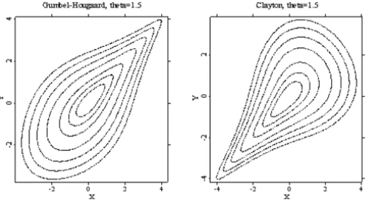
Figure 4.6 represents the countour diagrams of the Gumbel-Hougaard and Clayton copulae with parameter θ= 1.5.

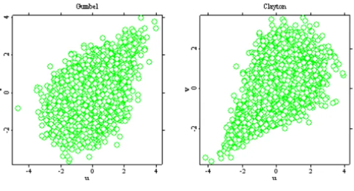
Recall that the Gumbel-Hougaard copula generates an upper tail dependence and the Clayton copula is able to model a lower tail dependence. Figure 4.7 represents an example of Gumbel-Hougaard and Clayton copulae sampling with fixed marginal parametersσ₁ = 1, σ₂ = 1 and θ = 1.5.

(26)

4 Examples

Figure 4.5. Density of a Clayton copula with θ= 1.5

clayton.xpl

Figure 4.6. Contour plots of the Gumbel-Hougaard and Clayton copulae, θ = 1.5 ghccont.xpl

(27)

4 Examples

Figure 4.7. 10000-sample output with fixedσ₁ = 1, σ₂ = 1of the Gumbel-Hougaard and Clayton copulae, θ= 1.5

ghcsampleout.xpl

EXAMPLE 4.5. The function

C_θ(u, v) = uv

1−θ(1−u)(1−v) (4.11)

represents the Ali-Mikhail-Haq family of copulae,|θ| ≤1. If θ = 0, then we have an independence: C_θ(u, v) =C⁰. This family does not contain the Fréchet bounds. The density of an AMH copula with θ= 0.8 is represented by figure 4.8.

EXAMPLE 4.6. The Frank copula with dependence parameter 0 < θ ≤ ∞ is represented by the function:

C_θ(u, v) =−1 θlog

1 + (e^−θu−1)(e^−θv −1) (e^−θ−1)

(4.12) The dependence becomes maximal when θ tends to infinity and independence is achieved when θ = 0. The density of a Frank copula for the case of θ = 5.0 is given by figure 4.9.

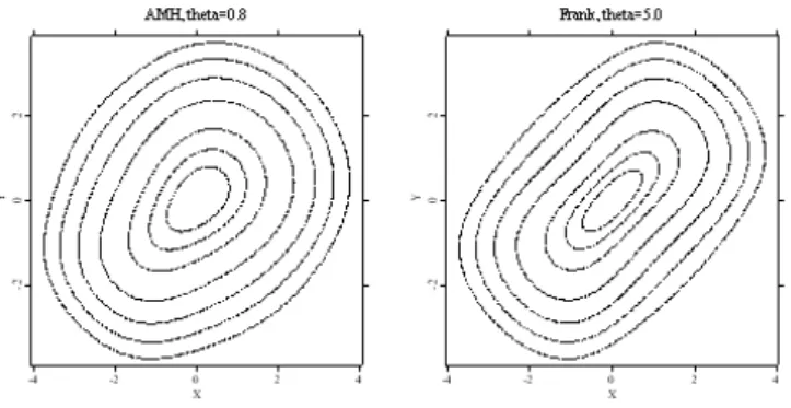
Figure 4.10 represents the countour diagrams of the Ali-Mikhail-Haq copula with parameterθ = 0.8 and of the Frank copula with parameter θ = 5.0.

Figure 4.11 represents an example of Ali-Mikhail-Haq and Frank copulae sampling with fixed marginal parameters σ₁ = 1,σ₂ = 1 and copulae dependence parameters of θ= 0.8 and θ = 5.0 respectively.

(28)

4 Examples

Figure 4.8. Density of a AMH copula with θ= 0.8

amh.xpl

Figure 4.9. Density of a Frank copula with θ= 5.0

frank.xpl

(29)

4 Examples

Figure 4.10. Contour plots of the AMH copula with θ= 0.8 and Frank copula with θ= 5.0

amhfcont.xpl

Figure 4.11. 10000-sample output with fixed σ₁ = 1, σ₂ = 1 of the AMH copula, θ= 0.8and Frank copula, θ = 5.0

amhfsampleout.xpl

(30)

4 Examples

Until now, we have considered copulae only in a 2-dimensional setting. Let us now extend this concept to the d-dimensional case, for a random variable in R^d with d≥1.

(31)

5 Multivariate copulae

Let U₁, U₂, ..., U_d be nonempty sets in R and consider the function F : U₁ ×U₂× ...×U_d−→R. For a= (a₁, a₂, ..., a_d) and b = (b₁, b₂, ..., b_d) with a≤b (i.e. a_k≤b_k for all k) let B = [a, b] = [a₁, b₁]×[a₂, b₂]×...×[a_n, b_n] be the d-box with vertices c= (c₁, c₂, ..., c_d). It is obvious, that each c_k is either equal to a_k or to b_k.

DEFINITION 5.1. The F-volume of a d-box B = [a, b] = [a₁, b₁]×[a₂, b₂]×...× [a_d, b_d]⊂U₁×U₂×...×U_d is defined as follows:

V_F(B) =

d

X

k=1

sgn(c_k)F(c_k) (5.1)

where sgn(c_k) = 1, if c_k =a_k for even k and sgn(c_k) = −1, if c_k=a_k for odd k.

EXAMPLE 5.1. For the case of d = 3, the F-volume of a 3-box B = [a, b] = [x₁, x₂]×[y₁, y₂]×[z₁, z₂] is defined as:

V_F(B) =F(x₂, y₂, z₂)−F(x₂, y₂, z₁)−F(x₂, y₁, z₂)−F(x₁, y₂, z₂) +F(x₂, y₁, z₁) +F(x₁, y₂, z₁) +F(x₁, y₁, z₂)−F(x₁, y₁, z₁)

DEFINITION 5.2. F is said to be a d-increasing function if for all d-boxes B with vertices in U₁×U₂ ×...×U_d holds:

V_F(B) ≥ 0 (5.2)

DEFINITION 5.3. If U1, U2, ..., Ud have a smallest element minU1, minU2,..., minU_d, respectively, then we say, that a function F : U₁ ×U₂×...×U_d −→ R is grounded if :

F(x) = 0 for all x∈U₁×U₂×...×U_d (5.3) such that x_k = minU_k for at least one k.

While the lemmas, which we have presented for the 2-dimensional case, have analogous multivariate versions (Nelsen, 1999), we will leave them out here.

DEFINITION 5.4. A d-dimensional copula (or d-copula) is a function C defined on the unit d-cube I^d=I×I×...×I such that

(32)

5 Multivariate copulae

• for every u∈I^d holds: C(u) = 0, if at least one coordinate of u is equal to 0;

i.e. C is grounded.

• for every a, b∈I^d with a≤b holds:

V_C([a, b]) ≥ 0; (5.4)

i.e. C is d-increasing.

• for every u∈I^d holds: C(u) = u_k, if all coordinates of u are 1 except u_k.

Analogously to the 2-dimensional setting, let us state Sklar’s theorem for the d- dimensional case.

THEOREM 5.1. Sklar’s Theorem:

If the marginals F₁, ...F_d of the multiveriate distribution function F are continuous, there exists a unique copula C : [0,1]^d→[0,1] such that

F(x₁, ..., x_d) =C{F_X₁(x₁), ..., F_X_d(x_d)} (5.5) Conversely, if Cis a copula andF_X₁, F_X₂, ..., F_X_d are distribution functions thenF defined by 5.5 is a d-dimensional distribution function with marginals F_X₁, F_X₂, ..., F_X_d.

If the densityf of F exists, one can derive the relationship between the densityf of F and c of C:

f(x₁, ..., x_d) =c{F_X₁(x₁), ..., F_X_d(x_d)}

d

Y

j=1

f_j(x_j) (5.6)

where the copula density is

c(u₁, ..., u_d) = ∂^dC(u₁, ..., u_d)

∂u1...∂ud

(5.7) and u_j =F_X_j(x_j),f_j(x_j) =F_X⁰

j(x_j).

In order to illustrate the d-copulae we present the following examples:

EXAMPLE 5.2. LetΦ denote the univariate standard normal distribution function and Φ_Σ,d the d-dimensional standard normal distribution function with correlation matrix Σ. Then a function

C^Gauss(u₁, ..., u_d,Σ) = Φ_Σ,d

Φ⁻¹(u₁), ...,Φ⁻¹(u_d)

=

Z φ⁻¹₁ (ud)

−∞

...

Z φ⁻¹₂ (u1)

−∞

f_Σ(x₁, ..., x_n)dx₁...dx_d (5.8)

(33)

5 Multivariate copulae

is a d-dim Gaussian copula. The density of the d-dim Gaussian copula is given by f₍u₁, ..., u_d,Σ) = ∂^dC(u1, ..., u_d)

∂u1, ..., ∂ud

= 1

pdet(Σ) ×

(5.9)

× exp

−(Φ⁻¹(u1), ...,Φ⁻¹(ud))⁰(Σ⁻¹− Id)(Φ⁻¹(u1), ...,Φ⁻¹(ud) 2

EXAMPLE 5.3. A d-dim Gumbel-Hougaard copula with dependence parameter θ from the interval[1,∞) is a function:

C_θ^GH(u₁, ..., u_d) = exp



−

( _d X

j=1

(−logu_j)^θ )^1/θ

 (5.10)

If θ= 1, Gumbel-Hougaard copula reduces to the d-dimensional product copula, i.e.

C₁(u₁, ..., u_d) =

d

Y

j=1

u_j = Π^d(u) (5.11)

EXAMPLE 5.4. A d-dim Frank copula with parameter θ >0 is given by

C_θ(u₁, ..., u_d) =−(1/θ) log (

1 + Qd

i=1(e^−θuⁱ−1) (e^−θ−1 )^d−1

)

(5.12) EXAMPLE 5.5. A d-dim Ali-Mikhail-Haq copula with −1≤θ <1 is defined by

Cθ(u1, ..., ud) =

Qd i=1u_i 1−θn

Qd

i=1(1−u_i)o (5.13)

EXAMPLE 5.6. A d-dim Clayton copula with copula dependence parameter θ >0 is given by

C_θ(u₁, ..., u_d) = (u^−θ₁ +...+u^−θ_d −d+ 1)^−1/θ (5.14) and its density function is

c_θ(u₁, ..., u_d) =

d

Y

j=1

{1 + (j−1)θ}

d

Y

j=1

u^−(θ+1)_j ( _d

X

j=1

u^−θ_j −d+ 1

)^−(1/θ+d)

(5.15)

(34)

6 Copulae estimation

Consider a vector of random variables: X = (X₁, ..., X_d)^T. Let F_X₁(x₁, δ₁),..., FX_d(xd, δd) denote the distribution functions of X1, ..., Xd. Recall from Sklar’s theorem, that we can write the following copula-based model for the distribution of the vector X:

F(x₁, ..., x_d;δ₁, ..., δ_d;θ) = C{F_X₁(x₁, δ₁), ..., F_X₂(x₂, δ₂);θ} (6.1) Suppose we want to estimate this model, i.e. we want to estimate the copula dependence parameter θ and the parameters from the marginals δ1, ..., δd.

Assume that the density of the copula C is given by c:

c(u1, ..., ud;θ) = ∂^dC(u₁, ..., u_d;θ)

∂u₁...∂u_d (6.2)

If the densityf of F exists, one can derive the following relationship between the densityf of F and c of C:

f(x₁, ..., x_d;δ₁, ..., δ_d;θ) =c{F_X₁(x₁, δ₁), ..., F_X_d(x_d, δ_d);θ}

d

Y

j=1

f_j(x_j;δ_j) (6.3)

Suppose that we have n i.i.d. d-dimensional vectors of observations (x₁, ..., x_n), i.e.

{x_i}ⁿ_i=1 with(x_1,i, ..., x_d,i)^T. The “full” likelihood function for {x_i}ⁿ_i=1 is then given by

L(x₁, ..., x_d;δ₁, ..., δ_d;θ) =

n

Y

i=1

f(x_1,i, ..., x_d,i;δ₁, ..., δ_d;θ) (6.4) and the corresponding “full” log-likelihood function is given by

l(x₁, ..., x_d;δ₁, ..., δ_d;θ)

=

n

X

i=1

"

logc{F_X₁(x_1,i, δ₁), ..., F_X_d(x_d,i, δ_d);θ}+

d

X

j=1

logf_j(x_j,i;δ_j)

#

(6.5)

=

n

X

i=1

logc{F_X₁(x_1,i, δ₁), ..., F_X_d(x_d,i, δ_d);θ}+

n

X

i=1 d

X

j=1

logf_j(x_j,i;δ_j)

Our objective is to maximize this log-likelihood numerically.

(35)

6 Copulae estimation

6.1 Full maximum likelihood estimation

In the full maximum likelihood (FML) procedure the marginal parametersδ₁, ..., δ_d and the copula dependence parameterθ are estimated simultaneously. The estimates vector

δˆ₁, ...,δˆ_d,θˆT

is a solution of ∂l

∂δ₁, ..., ∂l

∂δ_d, ∂l

∂θ

= 0 (6.6)

The drawback of the FLM estimation is that with an increasing scale of the problem, the algorithm becomes too burdensome computationally.

6.2 The inference for margins method

In the inference for margins (IFM) method, the marginal parameters δ₁, ..., δ_d are estimated in the first step. The estimator of the copula dependence parameter is obtained in the second step by substituting δˆ₁, ...,δˆ_d in the “full” log-likelihood function and by numerical maximisation with respect to θ.

1. The estimates vector (δˆ₁, ...,δˆ_d) is obtained by maximising the log-likelihood function for each marginal:

l_j(δ_j) =

n

X

i=1

f_j(x_j,i;δ_j) for j = 1, ..., d, (6.7) i.e. for j = 1, ..., d the estimates are given by

δˆ_j = arg max

δ l_j(δ_j) (6.8)

2. Substitute these marginal estimates in the “full” log-likelihood and maximize l(ˆδ₁, ...,δˆ_d;θ) =

n

X

i=1

lncn

F_X₁(x₁,δˆ₁), ..., F_X_d(x_d,δˆ_d);θo

(6.9) with respect toθ, i.e. the estimator of the copula dependence parameter θ is given by

θˆ= arg max

θ l(ˆδ1, ...,δˆd;θ) (6.10)

(36)

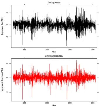
Figure 6.1.Dax and Dow Jones log-returns for the period January 1, 1997 to March 20, 2004 (1573 observations).

daxdowlogreturns.xpl

6.3 Application of the IFM procedure

The IFM procedure is applied to daily observations of a portfolio consisting of the Dax and the Dow Jones for the period January 1, 1997 to March 20, 2004 (1823 observations). The log-returns are shown the picture 6.1. We consider a moving time window with n= 250 observations, i.e. the parameter estimates at each point are obtained from the last250 observations. The univariate margins (log-returns) are assumed to be normally distibuted X_j,i ∼ N(0, σ²_j), j = 1,2 with parameters δ_j =σ_j² estimated from the data. Figure 6.2 and 6.3 represent the density of the Dax and Dow Jones respectively, estimated nonparametrically using Quartic kernel with bh= 1.06bσn⁻¹⁵.

To make procedure running, we have to specify the copula function. Selected copula belongs to the Gumbel-Hougaard family of copulae:

C_θ^GH(u, v) = exp

−n

(−logu)^θ+ (−logv)^θo1/θ

(6.11) Recall, that for this copula parameter θ may take values in the interval [1,∞).

Independence is achieved ifθ = 1.

According to the IFM procedure, we estimate at first parameters from the marginal distributions. Figure 6.4 represents estimates of parametersδ₁ from the Dax and

(37)

Figure 6.2.Density of the Dax log-returns (red) and normal density (black), estimated nonparametrically using Quartic kernel withbh= 1.06bσn⁻¹⁵ .

kernelest.xpl

Figure 6.3.Density of the Dow Jones log-returns (blue) and normal density (black), estimated nonparametrically using Quartic kernel with bh= 1.06bσn⁻¹⁵ .

kernelest.xpl

(38)

min max mean median std error

δˆ₁ 0.013345 0.029246 0.018396 0.017827 0.0042519 δˆ₂ 0.008681 0.016996 0.012817 0.012586 0.0017591 θˆ 1 1.12866 1.033 0.0195815 0.034162

Table 6.1. Descriptive statistics for δˆ₁, δˆ₂,θˆ

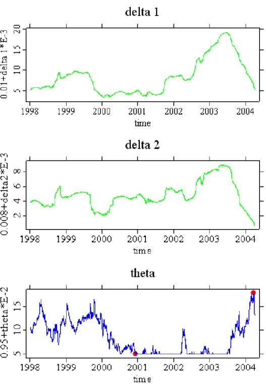
δ2 from the Dow Jones log-returns (upper respectively middle panel) and copula dependence parameter θ between Dax and Dow Jones log-returns (lower panel).

Descriptive statistics forδˆ₁, δˆ₂ and θˆare given by the table 6.1.

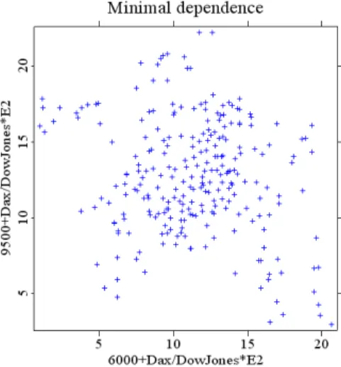
Estimates of the copula dependence parameter θ reaches its minimum equal to 1, which indicates independence for the Gumbel-Hougaard copula, at the time point corresponding to November 30, 2000. The maximum is reached at the time point corresponding to March 11, 2004. Figures 6.5 and 6.6 represent the last 250 realizations of the Dax and Dow Jones log returns, corresponding to minimal (November 30, 2000) and maximal (March 11, 2004) dependence.

(39)

Figure 6.4.Parameters δˆ1 and δˆ2 estimated from normal marginals of the Dax and Dow Jones log-returns (upper respectively middle panel) and estimated copula dependence parameter θˆ(lower panel). The resultes are obtained using IFM method with moving time window n= 250.

delta12thetaIFM.xpl

(40)

Figure 6.5.Dax and Dow Jones log-returns at minimal dependence (November 30, 2000).

maxmindep.xpl

Figure 6.6.Dax and Dow Jones log-returns at maximal dependence (March 11, 2004).

maxmindep.xpl

(41)

7 Adaptive copulae estimation

In this part we discuss a new procedure for estimating the copula dependence parameterθ using adaptive techniques. The approached, called local change point analysis(LCPD) (Mercurio, Spokoiny, 2004), is based on the assumption of local time homogeneity, i.e. for every moment n there is exists a historic time interval [n−m, n[, in which the copula parameter θ is nearly constant. Our main objective is therefore to describe the interval of homogeneity and to estimate copula dependence parameterθ_n from this interval.

7.1 Choice of the interval of homogeneity

The approach is based on the adaptive choice of the interval of homogeneity for the endpoint n. This choice is done by using local change point detection (LCPD) algorithm. One defines a family of intervals of the formI ={I_k, k = 0,1, ...} such that I_k = [n−m_k, n]with m_k: m₀ < m₁ < m₂ < ...≤n. Thus, the intervals I_k are ordered by their length m_k.

The LCPD procedure is made up by the following parts:

1. start from the smallest interval I₀

2. test the hypothesis of homogeneity withinI0

3. if the hypothesis is not rejected, take the next larger interval

4. continue the procedure until change point bν is detected or the largest possible interval [0, n[ is reached

5. if the hypothesis of homogeneity within some I_k is rejected, the estimated interval of homogeneity is given by Ib= [bν, n[, otherwise we take Ib= [0, n[

6. estimate the copula dependence parameter θ from observation S_t for t ∈ I,b assuming the homogeneous model within I, i.e. defineb θb_n =θe_I_b

To make the procedure running, we have to perform the homogeneity test.