Analysis with Applications to
Modeling Time Series and Panel Data
Inauguraldissertation zur
Erlangung des Doktorgrades der
Wirtschafts- und Sozialwissenschaftlichen Fakultät der
Universität zu Köln
2013
vorgelegt von
Dipl.-Vw. Dominik Liebl
aus
Passau
Referent: Prof. Dr. Karl Mosler (Universität zu Köln) Korreferent: Prof. Dr. Alois Kneip (Universität Bonn) Tag der Promotion: 21. Aug. 2013
Contents i
List of Figures v
Introduction 1
1 Modeling and Forecasting Electricity Spot Prices: A Functional
Data Perspective 7
1.1 Introduction . . . . 8
1.2 Electricity data . . . . 12
1.3 Functional factor model . . . . 16
1.4 Estimation procedure . . . . 18
1.4.1 Estimation of the price-demand functions Xt . . . . 19
1.4.2 Estimation of the basis system {f1, . . . , fT} . . . . 20
1.4.3 Random domains D(Xt) = [at, bt] . . . . 22
1.4.4 The estimator {fˆ1, . . . ,fˆK} . . . . 23
1.4.5 A note on convergence . . . . 24
1.5 Application . . . . 26
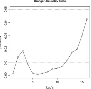
1.5.1 Interpretation of the factors and exemplary analysis of the scores . . . . 29
1.5.2 Validation of the model assumptions . . . . 30
1.6 Forecasting . . . . 32
1.6.1 Forecasting with the FFM . . . . 32
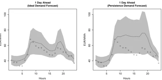
1.6.2 Competing forecast models . . . . 35
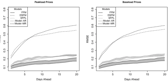
1.6.3 Evaluation of forecast performances . . . . 39
i
1.7 Conclusion . . . . 43
2 A fundamental model for electricity spot prices using functional data analysis 45 2.1 Introduction . . . . 45
2.2 Data . . . . 51
2.3 Model & estimators . . . . 52
2.3.1 Unifying regression model . . . . 56
2.3.2 The estimator . . . . 59
2.3.3 Random design of the prediction points . . . . 60
2.3.4 Boundary estimators . . . . 62
2.4 Technical assumptions & main results . . . . 64
2.4.1 Optimal bandwidth selection . . . . 69
2.4.2 Estimation of the eigencomponents . . . . 70
2.4.3 Estimation of the principal component scores . . . . 71
2.5 Application . . . . 74
2.6 Conclusion . . . . 81
2.7 Appendix: Proofs . . . . 82
2.7.1 Proof of Proposition 2.4.1 . . . . 82
2.7.2 Proof of Theorem 2.4.1 . . . . 82
2.7.3 Proof of Theorem 2.4.2 . . . . 90
3 The R-package phtt: Panel Data Analysis with Heterogeneous Time Trends 95 3.1 Introduction . . . . 95
3.2 Panel models for heterogeneity in time trends . . . 100
3.2.1 Computational details . . . 103
3.2.2 Application . . . 105
3.3 Panel criteria for selecting the number of factors . . . 108
3.3.1 Application . . . 111
3.4 Panel models with stationary common factors . . . 115
3.4.1 Model with known number of factors d . . . 115
3.4.2 Model with unknown number of factors d . . . 116
3.4.3 Application . . . 119 3.5 Models with additive and interactive unobserved effects . . . 122 3.5.1 Specification tests . . . 125 3.5.1.1 Testing the sufficiency of classical additive effects 126 3.5.1.2 Testing the existence of common factors . . . 128 3.6 Interpretation . . . 130 3.7 Summary . . . 133
Conclusions 135
Danksagung 139
References 141
1.1 Time series of electricity market data . . . . 10
1.2 Univariate time series of fitted price-demand functions . . . . 13
1.3 Empirical covariance function and VARIMAX rotated basis functions 28 1.4 Time series of principal component scores . . . . 28
1.5 P-values of Granger-causality tests . . . . 30
1.6 Hourly electricity spot prices . . . . 33
1.7 Forecast of the price-demand function of January 25, 2008 . . . . 34
1.8 Comparison of the spot prices and the 1 day ahead forecasts . . . 36
1.9 Root mean squared errors . . . . 41
1.10 Mean and trimmed mean values of the interval scoresSαint(h, `) . . 42
2.1 Discretization points of the random price functions . . . . 47
2.2 Scatter plot of prediction points . . . . 49
2.3 Contour plots of the estimated mean functions . . . . 75
2.4 First and second eigenfunctions . . . . 77
2.5 Temperature dependent variance shares . . . . 78
2.6 Fitted price functions . . . . 80
3.1 Plots of the dependent variable and the regressor variables . . . . 100
3.2 Estimated factors and time-varying individual effects . . . 108
3.3 Scree plot produced by the plot()-method . . . 114
3.4 Estimated factors and time-varying individual effects . . . 122
3.5 Estimated common factors, time-, and individual-effects . . . 126
3.6 Visualization of the differences in the individual effects . . . 132
v
This thesis contributes to a specific branch of nonparametric statistics called
“functional data analysis”. While classical statistics deals with the analysis of random scalars, vectors, and matrices, functional data analysis (FDA) refers to the statistical analysis of random functions. Examples of random functions in- clude biological and biomechanical data, e.g., growth curves, which can be sam- pled (nearly) without noise at (in principle) arbitrary discretization points. This type of functional data was the motivating starting point for the development of suitable statistical methods [see Rao (1958) for an early reference].
The next generation of methods for functional data focuses on latent random functions from which we observe only finitely many, noisy discretization points—a situation typically encountered in economic contexts. Here, the functional nature of the data represents a qualitative assumption on the underlying data-generating process. Examples in the literature of this kind of functional data include the analysis of ebay auction prices, production indices, and implied volatility func- tions [see, e.g., Wang et al.(2008b), Ramsay & Ramsey (2002), and Benko et al.
(2009)].
The potentially infinite dimension of functional data demands for methods of dimensionality reduction in advance of almost any further statistical analysis.
In this regard, the functional version of principal components analysis (FPCA) became the de facto standard for decomposing random functions into useful basis components. The resulting decomposition of random functions into linear combi- nations of basis functions (called eigenfunctions) and univariate random variables (called scores), leads to the well-known Karhunen-Loève decomposition [see, e.g., Ash & Gardner (1975)]. The underlying idea is that of a function space with pairwise orthonormal basis functions. FPCA chooses basis functions, in an op-
1
timal way such that a low number of basis functions suffices to approximate the original random functions with high accuracy.
Nowadays many classical statistical models are generalized for the case of random functions and very often FPCA builds the core method that allows for this kind of generalization. Prominent examples are functional linear regression models, functional auto regressive models, and functional canonical correlation analysis [see Ramsay & Dalzell (1991), Bosq (2000) and He et al. (2003)]. How- ever, there are also statistical topics and problems exclusively encountered in FDA, such as the statistical analysis of differential equations and the problem of registration in the case of misaligned functions [see, e.g., Ramsay (1996) and Kneip & Ramsay (2008)]. An excellent overview of FDA methods can be found in the monographs of Ramsay & Silverman (2005) and Ferraty & Vieu (2006).
FPCA is well studied for the classical case, where it is assumed that a sample of functions is observed precisely; however, this is a situation rarely fulfilled in practice. Recent work focuses on the more realistic case of latent functional data with (finitely many) noisy discretization points per function.
Generally, there are two different strategies for conducting FPCA in these more challenging cases: First, one can either pre-smooth each function and then estimate the covariance function. Second, one can estimate the covariance func- tion directly from the noisy discretization points using nonparametric smoothing procedures. The former possibility is applied in Chapters 1 and 2, while the latter is used in Chapter 2.
The latter possibility has the further advantage that it also works for sparse functional data with only very few observations per function. But both strate- gies involve nonparametric smoothing procedures, and those procedures crucially depend on an appropriate choice of smoothing parameters. This problem is of particular interest and is carefully treated in all of the following chapters. Con- trary to the usual case, optimization has to be done with respect to the common basis (or eigen-)functions and not with respect to the single random functions.
In this thesis we focus on the following three classical statistical models and their application in the context of functional data analysis: Chapter 1 deals with the functional factor model, in Chapter 2 we introduce multivariate nonparamet- ric regression model as a tool for FPCA, and in Chapter 3 we discuss panel data
models that allow for functional factor structures in the error term.
In Chapter 1, we propose a new perspective on modeling and forecasting elec- tricity spot prices. Our approach is motivated by the data-generating process of electricity spot prices, which is well described what is called the merit order model. The merit order model is a micro economic model based on the assump- tion that spot prices on electricity exchanges are determined by the marginal generation costs of the last power plant that is required to cover the demand.
The resulting merit order curve reflects the increasing generation costs of the in- stalled power plants. Correspondingly, we suggest interpreting hourly electricity spot prices as noisy discretization points of smooth price functions.
These price functions are modeled by a functional factor model (FFM) for which we discuss a two-step estimation procedure. The first step is a classical pre-smoothing step in order to estimate the single price functions from the noisy discretization points. The second step then aims for a robust estimation of a finite set of common basis functions from the pre-smoothed price functions. In doing this, we carefully consider the issue of finding an optimal smoothing parameter.
The presentation of our functional factor model concludes with an extensive forecast study which compares our FFM with alternative time series models that have been successfully applied in the literature on electricity spot prices. The forecast study clearly confirms the superior power of our functional factor model and the use of price functions as underlying structures of electricity spot prices in general.
A slightly modified version of Chapter 1 is forthcoming as a single-authored article in The Annals of Applied Statistics; see Liebl (2013).
Chapter 2 further discusses the problem of modeling electricity spot prices.
On the one hand, we extend the concept of price function introduced in Chapter 1 by two additional covariables. On the other hand, we focus on a generally deeper theoretical consideration of the involved multivariate nonparametric regression model, which is used as a tool for FPCA.
We extend existing theoretical results with respect to FPCA for sparse func- tional data by considering the asymptotic bias and variance of the multivariate local linear estimator of the mean and the covariance functions. Here, we carefully consider the effects of between-correlations, which are caused by the time series
context, and the effects of within-correlations, which are caused by the functional nature of the data.
In order to demonstrate the usefulness of our model we analyze the effects of Germany’s nuclear moratorium on March 14, 2011. This event describes a natural experiment, since in the course of Germany’s nuclear moratorium on March 14, 2011, eight nuclear power plants were phased out [Nestle (2012)]. The data set analyzed in Chapter 2 covers exactly one year before and one year after Germany’s nuclear power phase-out. We apply our model separately to these two time spans in order to contrast the different market situations.
Chapter 2 is based on a joint research project together with Prof. Dr. Alois Kneip (University Bonn). All paperwork as well as theoretical work is done by the author of this thesis, Prof. Dr. Alois Kneip checks plausibility of the theoretical work.
In Chapter 3 we pick up the successful application of FDA within the literature on panel data models. Recent panel data models allow us to control for complex unobserved heterogeneity effects by the incorporation of latent factor models.
This new kind of panel data models extends the classical concept of individual random (scalar) effects to random processes or random functions [see, e.g., Bai et al.(2009), Bai (2009), and Kneip et al. (2012a)].
Even though this class of panel models is of high relevance for practical prob- lems such as stochastic frontier analysis, they are still rarely applied in the empir- ical literature. Our implementation of these methods in the statistical software package of Bada & Liebl (2013b) provides a first step towards facilitating their application. Beyond this, we solve some open estimation problems, extend the suggested models for classical fixed effects, and introduce a new Hausman-type specification test.
As the estimation procedure of Kneip et al. (2012a) involves nonparametric smoothing methods, the choice of a reliable procedure to find an optimal smooth- ing parameter is most important for implementing the estimation procedure in a statistical software package. We consider this problem and suggest using Gen- eralized Cross Validation (GCV) in order to determine an upper bound for the optimal smoothing parameter. However, it is impossible to apply the classical GCV formulas as proposed, e.g., in Craven & Wahba (1978) since we do not
know the parameters β and vi(t). Our computational algorithm for determin- ing the GCV smoothing parameter is based on the parameter cascading method suggested in Cao & Ramsay (2010).
This GCV smoothing parameter builds an upper bound for the optimal smooth- ing parameter, since it does not account for the qualitative assumption of an un- derlying factor structure. The final optimal smoothing parameter lies somewhere between the GCV smoothing parameter and zero. Knowledge of this interval allows for a reasonable implementation of the computationally costly cross vali- dation criterion.
A slightly modified version of Chapter 3 is accepted as a co-authored article for the Journal of Statistical Software; see Bada & Liebl (2013a). The main sections of this article are Section 3.2, which describe the implementation of the estimation procedures proposed by Kneip et al. (2012a), and Section 3.4, which describe the implementation of the estimation procedures proposed in Bai (2009). The author of this thesis is responsible for Section 3.2, while the co-author of the article, Oualid Bada (Univeristy Bonn), is responsible for Section 3.4. Sections 3.3 and 3.5 discuss further estimation problems, model extensions, as well as specification tests. Generally speaking, those parts, which refer to the panel model of Kneip et al. (2012a) are written by the author of this thesis, those parts, which refer to the panel model of Bai (2009), are written by the co-author. The remaining parts of the latter sections, which refer to both models, as well as the introductory and the concluding Sections 3.1 and 3.6 are joint works of both authors.
The outline of this thesis is as follows: In Chapter 1 we present our perspective on modeling and forecasting electricity spot prices. In Sections 2.3 and 1.2 we motivate the conceptual idea and discuss peculiarities of electricity market data.
In Sections 1.3 and 1.4 we introduce the functional factor model and the two step estimation procedure. Chapter 1 is completed by an application of the model in Section 1.5 and a forecast study in Section 1.6. The results are discussed in Section 1.7.
In Chapter 2 we introduce multivariate nonparametric regression as a tool for FPCA. In Sections 2.1 and 2.2 we discuss the general ideas and the data. The nonparametric regression models as well as the multivariate local linear estimator are discussed in Section 2.3. In Section 2.4 we present our main theoretical results.
In Section 2.5 we apply the procedures to real data. Chapter 2 completed by the conclusion in Section 2.6.
In Chapter 3 we introduce our statistical software package Bada & Liebl (2013b). Section 3.1 discusses the implemented panel data models at a general level. In Sections 3.2 and 3.4 the models are discussed in more detail. In Section 3.3 we present several criteria to determine the factor dimension. In Section 3.5 we augment the panel data models for classical fixed effects and propose a Hausman-type specification test. In Section 3.6 we outline an example of the application of the procedures. Chapter 3 is completed by a short summary in Section 3.7.
Modeling and Forecasting Electricity Spot Prices: A Functional Data Perspective
Classical time series models have serious difficulties in modeling and forecast- ing the enormous fluctuations of electricity spot prices. Markov regime switch models belong to the most often used models in the electricity literature. These models try to capture the fluctuations of electricity spot prices by using different regimes, each with its own mean and covariance structure. Usually one regime is dedicated to moderate prices and another is dedicated to high prices. However, these models show poor performance and there is no theoretical justification for this kind of classification. The merit order model however, the most important micro-economic pricing model for electricity spot prices, suggests a continuum of mean levels with a functional dependence on electricity demand.
We propose a new statistical perspective on modeling and forecasting elec- tricity spot prices that accounts for the merit order model. In a first step, the functional relation between electricity spot prices and electricity demand is mod- eled by daily price-demand functions. In a second step, we parameterize the series of daily price-demand functions using a functional factor model. The power of this new perspective is demonstrated by a forecast study that compares our func- tional factor model with two established classical time series models as well as
7
two alternative functional data models.
1.1 Introduction
Time series of hourly electricity spot prices have peculiar properties. They differ substantially from time series of equities and other commodities because elec- tricity still cannot be stored efficiently and, therefore, electricity demand has an untempered effect on the electricity spot price [Knittel & Roberts (2005)].
The development of models for electricity spot prices was triggered by the liberalization of electricity markets in the early 1990s. Hourly electricity spot prices are usually considered to be multivariate (24-dimensional) time series since for each day t the 24 intra-day spot prices are settled simultaneously the day before [Huisman et al. (2007)].
However, classical time series models adopted for electricity spot prices such as autoregressive, jump diffusion, or Markov regime switch models reduce the multivariate time series to univariate time series either by taking daily averages of the 24 hourly spot prices [Weron et al. (2004), Kosater & Mosler (2006), and Koopmanet al. (2007)] or by considering each hourhseparately [Karakatsani &
Bunn (2008)]. These unnatural aggregations and separations of the data neces- sarily come with great losses in information.
Our model, a functional factor model (FFM), is not a mere adaption of a classical time series model but is motivated by the data-generating process of electricity spot prices itself. Pricing in power markets is explained by the merit order model. This model assumes that the spot prices at electricity exchanges are based on the marginal generation costs of the last power plant that is required to cover the demand. The resulting so-called merit order curve reflects the increasing generation costs of the installed power plants. Often, nuclear and lignite plants cover the minimal demand for electricity. Higher demand is mostly served by hard coal and gas fired power plants.
Due to its importance the merit order model is referred to as a fundamental market model [Burgeret al. (2008), Chapter 4]. Essentially, the consideration of this fundamental model yields to the superior forecast performance of our FFM in comparison to state of the art time series models and alternative functional
data models.
It is important to emphasize that the merit order model is not a static model.
The merit order curve rather depends on the variations of the daily prices for raw materials, the prices of CO2 certificates, the weather, plant outages, and maintenance schedules of power plants.
The merit order curve is most important for the explanation of electricity spot prices in the literature on energy economics and justifies our view on the set of hourly electricity spot prices {yt1, . . . , yt24} of day t. We do not interpret them as 24-dimensional vectors but rather as noisy discretization points of a smooth price-demand function Xt, which can be formalized as follows:
yth = Xt(uth) +εth,
where uth denotes electricity demand at hourh of dayt and εth is assumed to be a white noise process.
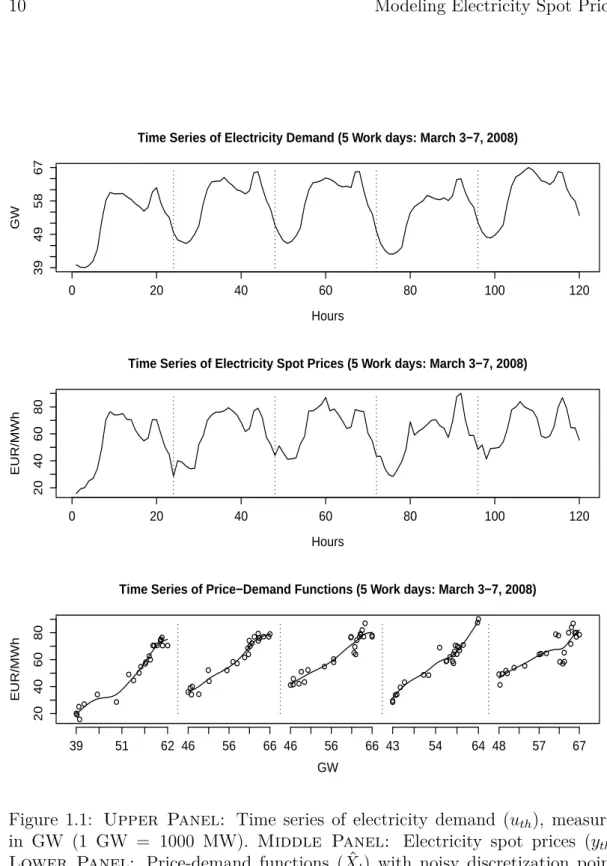
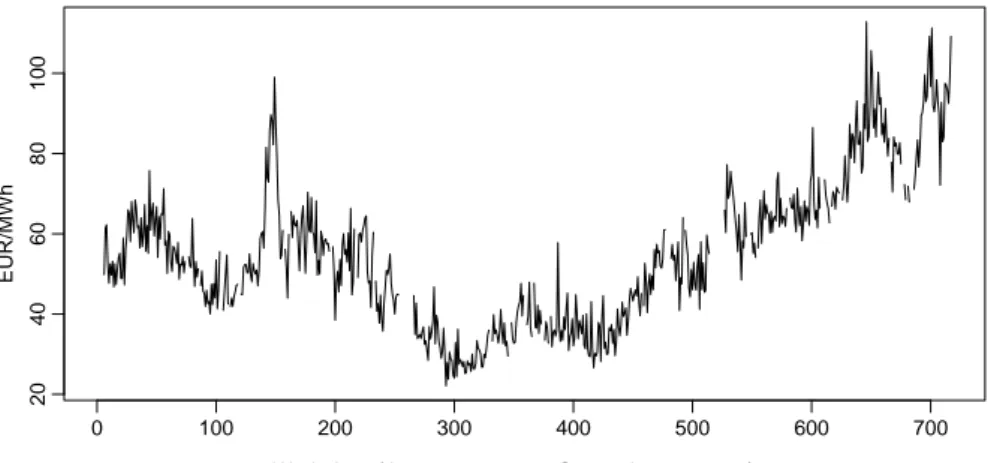
The price-demand function Xt(u) can be seen as the empirical counterpart of the merit order curve estimated non-parametrically from the N = 24 hourly price-demand data pairs (yt1, ut1), . . . ,(ytN, utN). Five exemplary estimated price- demand functions ˆXt(u) are shown in the lower panel of Figure 1.1. Figure 1.2 visualizes the temporal evolution of the time series of price-demand functions by showing the univariate time series ˆX1(u), . . . ,XˆT(u) for a fixed value of electricity- demand u= 58,000 MW for the whole observed time span ofT = 717 work days (Mo.-Fr.) from January 1, 2006 to September 30, 2008.
In order to capture the dynamic component of the price-demand functions we assume them to be generated by a functional factor model defined as
Xt(u) =
K
X
k=1
βtkfk(u),
where the factors or basis functions fk are time constant and the corresponding scores βtk are allowed to be non-stationary time series.
We do not specify a constant mean function in our FFM, since we allow the time series of price-demand functions (Xt(u)) to be non-stationary. Consequently, the classical interpretation of the factors fk as perturbations of the mean does
Time Series of Electricity Demand (5 Work days: March 3−7, 2008)
Hours
GW
0 20 40 60 80 100 120
39495867
Time Series of Electricity Spot Prices (5 Work days: March 3−7, 2008)
Hours
EUR/MWh
0 20 40 60 80 100 120
20406080
Time Series of Price−Demand Functions (5 Work days: March 3−7, 2008)
GW EUR/MWh 20406080
●●
●
●
●
●
●
●
●
●
●●●●●
●●●●●●●
●●
39 51 62 46 56 66 46 56 66 43 54 64 48 57 67
●●
●
●
●
●
●
●
●●●
●
●
●
●●
●●
●●●●●●
●●
●●
●
●
● ●
●●
●●
●●
●
●●●●●
●
●
●●
●●
●●
●● ●●
●
●
●●
●
●
●
●●
●
●●●●
●●
●
●
●●●● ●
●●●
●●
●●
●
●
●
●
●●
●●
●●
Figure 1.1: Upper Panel: Time series of electricity demand (uth), measured in GW (1 GW = 1000 MW). Middle Panel: Electricity spot prices (yth).
Lower Panel: Price-demand functions ( ˆXt) with noisy discretization points (yt1, ut1), . . . ,(ytN, utN).
not apply—as common in the literature on dynamic (functional) factor models;
see, e.g., Hays et al. (2012).
Note that the five price-demand functions in the lower panel of Figure 1.1 are observed on different domains. This distinguishes our functional data set from classical functional data sets, where all functions are observed on a common domain. We refer to this feature as random domains and its consideration in Sections 1.4.3 and 1.4.5 is a central part of our estimation procedure.
We use a two-step estimation procedure. The first step is to estimate the daily price-demand functions ˆXt by cubic spline smoothing for all days t∈ {1, . . . , T}.
The second step is to determine a K <∞ dimensional common functional basis system {f1, . . . , fK}for the estimated price-demand functions ˆX1, . . . ,XˆT. Given this system of basis functions we model the estimated daily price-demand func- tions by a functional factor model—using the basis functions as common factors.
The fitted discrete hourly electricity spot prices ˆyth are then obtained through the evaluation of the modeled price-demand functions at the corresponding hourly values of demand for electricity; formally written as: ˆyth = ˆXt(uth).
Functional data analysis (FDA) can share our perspective on electricity spot prices. A broad overview of many different FDA methods can be found in the monographs of Ramsay & Silverman (2005) and Ferraty & Vieu (2006). Particu- larly, Chapter 8 in Ramsay & Silverman (2005) and the non-parametric methods for computing the empirical covariance function as proposed in Staniswalis & Lee (1998), Yao et al.(2005), Hallet al.(2006), and Li & Hsing (2010) are important methodological references for this paper.
The application of models from the functional data literature to electricity market data is not new. For example, there is a vast literature on modeling and forecasting electricitydemand; see, e.g., Ferraty & Vieu (2006) and Antochet al.
(2010). However, modeling and forecasting electricity spot prices is much more difficult than modeling and forecasting electricity demand. The semi-functional partial linear model (SFPL) of Vilar et al. (2012) is one of the very rare cases in which FDA methods are used to forecast electricity spot prices.
Two very recent examples of other functional factor models are given by the functional factor analysis in Liu et al. (2012) and the functional dynamic factor model (FDFM) in Hays et al. (2012). Liu et al. (2012) propose a new rotation
scheme for the functional basis components. Hays et al. (2012) model a time series of yield curves and estimate their model by the EM algorithm. In contrast to the FDFM of Hayset al. (2012) we do not have to make a priori assumptions on the stochastic properties of the time series of scores in order to estimate our model components. Furthermore, we are able to model and forecast functional time series observed on random domains.
Very close to the FDFM of Hayset al. (2012) is the Dynamic Semiparametric Factor Model (DSFM) of Parket al. (2009). As our functional factor model the DSFM does not need a priori assumptions on the time series of scores. This and the fact that the DSFM was already successfully applied to electricity prices [Borak & Weron (2008) and Härdle & Trück (2010)] makes the DSFM a perfect competitor for our FFM.
The main difference between the FDFM of Hays et al.(2012) and the DSFM of Park et al. (2009) in comparison to our FFM is that the FFM can deal with functional times series observed on random domains. Furthermore, Park et al.
(2009) use an iterating optimization algorithm to estimate the basis functions of the DSFM, whereas we standardize the elements of the time series (Xt) so that we can robustly estimate the basis functions by functional principal component analysis. Our estimation procedure is much simpler to implement and faster with respect to computational time than the Newton-Raphson algorithm suggested in Park et al. (2009).
The next section is devoted to the introduction of our data set and to a critical consideration of the stylized facts of electricity spot prices usually claimed in the electricity literature. In Section 1.3 we present our functional factor model and in Section 1.4 its estimation. An application of the model to real data is presented in Section 1.5. Finally, the performance of the functional factor model is demonstrated by an extensive forecast study in Section 1.6.
1.2 Electricity data
We demonstrate our functional factor model by modeling and forecasting elec- tricity spot prices of the German power market traded at the European Energy Exchange (EEX) in Leipzig. The German power market is the biggest power
0 100 200 300 400 500 600 700 Work days (January 1, 2006 − September 30, 2008)
20406080100
EUR/MWh
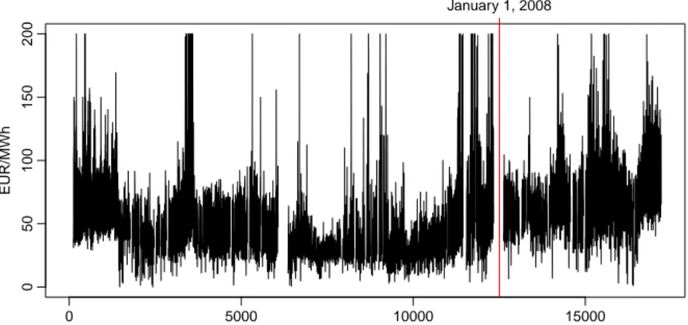
Figure 1.2: Univariate time series of fitted price-demand functions Xˆ1(u), . . . ,XˆT(u) evaluated at u= 58000 MW. Gaps correspond to holidays.
market in Europe in terms of consumption. The wholesale market is fragmented into an Over The Counter (OTC) market and the EEX. While the OTC mar- ket has a continuous trade, the EEX has a single uniform price auction with a gate closure for the day ahead market at 12 p.m. the day before physical deliv- ery. Although three-fourths of the trading volume is settled via bilateral OTC contracts, the EEX spot price is of fundamental importance as benchmark and reference point for other markets, such as OTC or forward markets [Ockenfels et al. (2008), Chapter 1].
The data for this analysis stem from three different publicly available sources.
The hourly spot prices of the German electricity market are provided by the European Energy Exchange (www.eex.com), hourly values of Germany’s gross electricity demand are provided by the European Network of Transmission System Operators for Electricity (www.entsoe.eu), and German wind power infeed data are provided by the EEX Transparency Platform (www.transparency.eex.com).
In the German electricity market, as in most of the electricity markets in the world, renewable energy sources are usually provided with purchase guarantees.
Therefore, not the hourly values of gross electricity demand are relevant for the pricing at the EEX but rather the hourly values of gross demand minus the hourly electricity infeeds from renewable energy sources. We consider only wind
power infeed data since the influences of other renewable energy sources such as photovoltaic and biomass on electricity spot prices are still negligible for the German electricity market (and their explicit consideration essentially would lead to the same results).
The data consists of pairs (yth, uth) withyth denoting the electricity spot price and uth the electricity demand of hour h ∈ {1, . . . ,24} at day t. We define electricity demanduth as the gross electricity demand of hour h and day t minus the wind power infeed of electricity at the corresponding hour h and day t.
The data set analyzed in this article covers T = 717 work days (Mo.-Fr.) within the time horizon from January 1, 2006 to September 30, 2008. For the sake of clarity, only working days are considered in our analysis since for weekends there are different compositions of the power plant portfolio. The same reasoning applies to holidays and so-called Brückentage, which are extra days off that bridge single working days between a bank holiday and the weekend. Therefore we set all holidays and Brückentage to NA-values.
As a referee noted, the time span of our data set is peculiar. Starting around January, 2007 a price bubble for raw commodities such as coal and gas was formed, which induced a strong increase in the electricity spot prices. Interestingly, the increase in the electricity spot prices is hardly visible in the original time series as shown in Figure 1.6. But it catches the eye in the plot of Figure 1.2, which shows the time series of price-demand functions ( ˆXt(u)|u) evaluated for a certain value of electricity demandu= 58,000 MW. The reason is that at this relatively high value of electricity demand usually coal and gas fired power plants cover the demand.
Very few (only 0.5%) of the data pairs (yth, uth) with pricesyth>200 EUR/MWh have to be treated as outliers since they cannot be explained by the merit order model. Even in exceptional situations the marginal costs of electricity produc- tion do not exceed the value of 200 EUR/MWh. Prices above this threshold are referred to as price spikes and have to be explained using an additional scarcity premium [Burger et al. (2008), Chapter 4]. The analysis of price spikes is a re- search topic on its own [Christensen et al.(2009)] and is not within the scope of this paper.
We exclude the outliers for the estimation of our model and denote the amount
of data pairs of day t used for estimation by Nt ≤ N = 24. Nevertheless, we use the whole data set, including the outliers, in order to assess the forecast performance of our model in Section 1.6.
Review: Stylized facts of electricity data Our functional perspective on electricity spot prices allows us to review critically the so-called “stylized facts”
of hourly electricity spot prices (yth). Usually, time series of electricity spot prices are assumed (i) to have deterministic daily, weekly and yearly seasonal patterns, (ii) to show price dependent volatilities, and (iii) to be stationary (after controlling for the seasonal patterns); see Huisman & De Jong (2003), Knittel
& Roberts (2005), Kosater & Mosler (2006), Huisman et al. (2007), and many others.
At first glance these stylized facts seem to be reasonable; see the middle panel in Figure 1.1. However, the first two stylized facts, (i) and (ii), are mislead- ing since both have their origins in the time series of electricity demand: the characteristics of electricity demand are rather carried over to the time series of electricity spot prices.
This can be explained by a micro-economic point of view, again using the merit order model. The merit order curve induces a monotone increasing sup- ply function for electricity, which implies higher electricity spot prices for higher values of electricity demand, where electricity demand can be considered as in- elastic. Given this micro-economic point of view, we can regard the daily supply functions for electricity as diffusers in the transmission from electricity demand uth to the electricity spot price yth.
Additional diffusion comes from the variations of the daily supply functions caused by the varying input-costs of, e.g., coal and gas. Compare to this the time series of electricity demand with the time series of electricity spot prices shown in the upper and middle panels of Figure 1.1 respectively. The seasonal patterns of electricity spot prices are just a diffused version of the smoother seasonal patterns of electricity demand.
Price dependent volatility (ii) can be explained by the slope of the merit order curve, which is increasing with electricity demand. Changes in electricity demand have greater price effects for greater values of electricity demand and therefore
cause greater volatilities than is the case for lower values of electricity demand.
Stationarity (iii) has to be considered critically, too. Recently, Bosco et al.
(2010) were able to show empirically that electricity spot prices at the EEX have a unit root. The authors point out that the stationarity assumption might be wrong in markets that are influenced by price-enhancing sources such as prices for coal and gas since time series of coal and gas prices are commonly found to be non-stationary. Our functional factor model allows for non-stationarity in the time series of price-demand functions (Xt) and, in fact, tests indicate that the estimated series of price-demand functions is non-stationary; see Section 1.5.2.
This short review of electricity spot prices demonstrates that electricity data are complex with dynamics induced by the variations of the merit order curve (mainly caused by varying input-costs) and separate additional dynamics induced by electricity demand. To the best of our knowledge, our functional factor model is the first model that allows for a separate consideration of these two stochastic sources. The variations dedicated to the dynamics of the merit order curve are captured by the price-demand functions and modeled by our functional factor model. The problem of modeling and forecasting electricity demand is “out- sourced” and the statistician can choose powerful specialized models for time series of gross electricity demand [Antoch et al. (2010)] and time series of wind power [Lau & McSharry (2010)]. This separation corresponds to the real data generating process.
1.3 Functional factor model
As mentioned above, electricity spot prices yt1, . . . , yt24 are actually one-day- ahead future prices since they are settled simultaneously at day t − 1. This implies that there is some degree of uncertainty about the next day world in the electricity spot priceyth, which we model non-parametrically as
yth = Xt(uth) +εth. (1.1) The error terms εth are assumed to be iid white noise errors with finite vari- ance V(εth) = σε2 and each function Xt is assumed to be continuous and square
integrable.
For each function Xt the values of electricity demand uth are only observed within random sub-domains D(Xt) = [at, bt], where [at, bt] ⊆ [A, B] ⊂ R. The unobserved univariate time series (at) and (bt) are assumed to be time series processes with A ≤ at < bt ≤ B and marginal pdf’s of at and bt given by fa(za)>0 and fb(zb)>0 for allza, zb ∈[A, B] and t ∈ {1, . . . , T}.
The price-demand functions are relatively homogeneous. All of them look very similar to the five randomly chosen price-demand functions shown in the lower panel of Figure 1.1. The underlying reason for this homogeneity is that, on the one hand, the merit order curve induces rather simple monotone increasing price- demand functions. On the other hand, the general portfolio of power plants, which is reflected by the merit order curve, is changing very slowly and can be considered as constant over the period of our analysis. We formalize this homogeneity of the price-demand functions by the assumption that the time series of price-demand functions (Xt) is generated by a functional factor model with time constant basis functions.
Given this assumption, every price-demand function Xt can be modeled by the same set of K < ∞ (unobserved) basis functions f1, . . . , fk, . . . , fK with fk ∈ L2[A, B], which span the K-dimensional functional space HK ⊂ L2[A, B]
such that we can write Xt(u) =
K
X
k=1
βtkfk(u) for all u∈[at, bt], (1.2) where the common basis functions fk as well as the scoresβtk are unobserved and have to be determined from the data. We use the usual orthonormal identifica- tion restrictions for the basis functions, which require that RABfk2(u)du = 1 and
RB
A fk(u)fl(u)du= 0 for all k < l∈ {1, . . . , K}.
The K real time series (βt1), . . . ,(βtK) are defined as
βt1 ... βtK
=
Rbt
at f12 · · · Rabt
t f1fK ... . .. ...
Rbt
at f1f2 · · · RabttfK2
−1
Rbt
at f1Xt ...
Rbt
at fKXt
(1.3)
and are allowed to be arbitrary non-stationary processes. Note that for at = A andbt=B the definition of the scoresβtk corresponds to the classical definition, given by βtk =RABXt(u)fk(u)du.
In the following section we propose an estimation algorithm for the functional factor model.
1.4 Estimation procedure
As outlined in Sections 2.3 and 1.2 we do not observe the series (Xt) directly but have to estimate each price-demand functionXtfrom the corresponding data pairs (yt1, ut1),. . .,(ytNt, utNt). After this initial estimation step, which is discussed in Section 1.4.1, we show in Section 1.4.2 how to determine an orthonormal K-dimensional basis system {f1, . . . , fK} for the classical functional data case when all price-demand functions X1, . . . , XT are observed on the deterministic domain D(Xt) = [A, B]. In Section 1.4.3 we generalize the determination of the orthonormalK-dimensional basis system{f1, . . . , fK} to our case, where the price-demand functionsXtare observed only on random domainsD(Xt) = [at, bt].
Finally, we define our estimator {fˆ1, . . . ,fˆK}in Section 1.4.4.
As usually for (functional) factor models, the set of factors {f1, . . . , fK} in Eq. (1.2) is only determined up to orthonormal rotations. Furthermore, the deter- mination of an orthonormalK-dimensional basis system {fˆ1, . . . ,fˆK}for a given series ( ˆXt) is, in the first instance, a mere algebraic problem. But it is also a sta- tistical estimation problem in the sense that ˆHK, with ˆHK = span( ˆf1, . . . ,fˆK), is a consistent estimator of the theoretical counterpartHK. The crucial assumption is thatXt comes from the FFM (1.2). Consistency of the estimation follows from the consistency of the single non-parametric estimators ˆXt(u), which converge in probability against Xt(u) as Nt → ∞ for all u ∈ [at, bt] and all t ∈ {1, . . . , T} [Benedetti (1977)]. Below in Section 1.4.5 we consider this issue in more detail.