Techniques to Implied Volatility
A Master Thesis Presented by
Zeng, Jin
(184784) to
Prof. Dr. Wolfgang H¨ ardle
CASE - Center of Applied Statistics and Economics Humboldt University, Berlin
in partial fulfillment of the requirements for the degree of
Master of Arts
I hereby confirm that I have authored this master thesis independently and without use of others than the indicated resources. All passages, which are literally or in gen- eral matter taken out of publications or other resources, are marked as such.
Zeng, Jin
Berlin, September 14, 2005
I would like to thank Professor Dr. Wolfgang H¨ardle for giving me the opportunity and motivation to write this thesis.
I’m especially indebted to Michal Benko for his excellent guidance all the time.
Furthermore I’m also grateful to my parents and my husband, without their support it would be impossible to finish this work.
Implied volatility is an important element in risk management and option pricing.
Black-Scholes model assumes a constant volatility, however, the evidence from financial market shows that the volatility is not constant but change with strike and time to maturity. In this paper, the time to maturity is fixed and we will construct the implied volatility function of strike or moneyness. We can use regression method for estimation, but the data from financial market contains some noise and we need to apply smoothing techniques to estimate this implied volatility function. The standard non- and semi- parametric regression methods don’t guarantee the resulting IV functions are arbitrage free, so we will insert our estimation result to Black and Scholes model and calculate the state price density (SPD). In a Black-Scholes model it is lognormal distribution with constant volatility parameter. In practice as volatility changes the distribution deviates from log-normality. We estimate volatilities and SPDs using EUREX option data on the DAX index by using different smoothing techniques. Our estimation will be carried out through the strike direction and moneyness direction. We will briefly introduce Local polynomials as one method. The most important smoothing techniques we will applied in this paper is B-splines, with the usage of roughness penalty, which allows a flexible choice on the degree of smoothness, and is promising for future research work on the arbitrage free constraint of implied volatility.
Keywords: implied volatility, state price density, B-splines, roughness penalty, linear differential operator
1 Introduction 11
2 The Implied Volatility and SPD 15
2.1 Statistical Properties of Implied Volatility . . . 15
2.2 Calculation the Implied Volatility . . . 16
2.3 State Price Density . . . 17
2.4 SPD estimation based on IV smile . . . 20
2.5 The Quantlet spdcal and spdcalm . . . 23
2.6 Arbitrage Free Constraint . . . 24
3 Nadaraya-Watson and Local Polynomial Estimator 26 4 Smoothing IV With Functional Data Approach 33 4.1 Basic Setup . . . 33
4.2 The Basis Function Approach . . . 34
4.3 B-spline Bases . . . 35
4.4 Estimation of Coefficients . . . 36
4.5 Choice of the Smoothing Parameter . . . 37
4.6 The Quantlet Bfacv and Bfagcv . . . 39
5 The Implemention of Penalized B-splines on Financial Market Data 42 5.1 Construction of the Model . . . 42
5.2 Volatility Smile as Function of Strike . . . 43
5.3 Multiple Observations . . . 55
5.4 Volatility Smile as Function of Moneyness I . . . 58
5.5 Volatility Smile as Function of Moneyness II . . . 61
5.6 Conclusions . . . 64
6 Summary and Outlooks 65 7 Appendix 66 7.1 XploRe quantlet lists . . . 66
7.1.1 Statistical Tools . . . 66
7.1.2 Implemention Examples . . . 71
7.2 Proofs . . . 76
7.2.1 Convexity of Call Price Function . . . 76
7.2.2 No Arbitrage Bounds of IV Smile . . . 77
1.1 DAX option on 2003-02-25, Implied volatility with respect to strike and maturity . . . 13 2.1 DAX option on 25th Feb, 2003,τ = 0.14167. Top panel: IV VS strike;
bottom: IV vs moneyness . . . 18 3.1 IV smile with strike, DAX call option,02-25-03, τ = 0.14167. Up-
per panel: Bandwidth=150, lower panel: Bandwidth=250. Nadaraya- Watson estimator is used. . . 29 3.2 IV smile with moneyness, DAX call option,02-25-03, τ= 0.14167. Up-
per panel: Bandwidth=0.05, lower panel: Bandwidth=0.1. Nadaraya- Watson estimator is used. . . 30 3.3 DAX call option,02-25-03, τ = 0.14167. Upper panel: IV smile with
strike, right panel: SPD. Bandwidth h= 700, the second order local polynomials is used. . . 31 3.4 DAX call option,02-25-03, τ = 0.14167. Upper panel: IV smile with
strike, right panel: SPD. bandwidth h = 0.4, the second order local polynomials is used. . . 32 5.1 IV-Strike, DAX call option on 02-25-03, tau=0.14167, Top: IV smile.
Bottom: SPD, red horizon line represents 0. Left: 4th order b-spline, right: 6th order B-spline . . . 44 5.2 DAX call option, 02-25-03, τ = 0.14167, L = D2, λ = 107, The blue
dashed horizontal line represents 0. . . 45 5.3 DAX call option, 02-25-03, τ = 0.14167, L = D2, λ = 108, The blue
dashed horizontal line represents 0. . . 46
5.4 DAX call option, 02-25-03, τ = 0.14167, L = D2, λ = 109, The blue dashed horizontal line represents 0. . . 47 5.5 DAX call option, 02-25-03, τ = 0.14167, L =D2, λ= 1014, The blue
dashed horizontal line represents 0. . . 48 5.6 DAX call option, 02-25-03, τ = 0.14167, L =D2, λ= 1016, The blue
dashed horizontal line represents 0. . . 49 5.7 DAX call option, 02-25-03, τ = 0.14167, L = D2, λ = 5×10²⁰, The
blue dashed horizontal line represents 0. . . 50 5.8 GCV score with respect to smoothing parameterλ, left panel: L=D2,
right panel: L=D3. . . 51 5.9 DAX call option, 02-25-03, τ= 0.14167, L=D2. Upper left panel: IV
smile with strike. Upper right panel: SPD (black thick line), log-normal distribution (blue thin line), red horizon line represents 0. Bottom left panel: first derivative of volatility with respect to strike. Bottom right panel: the first derivative (black line) and its no arbitrage bounds (red dashed line). . . 53 5.10 DAX call option, 02-25-03,τ= 0.14167, L=D3. Upper left panel: IV
smile with strike. Upper right panel: SPD (black thick line), log-normal distribution (blue thin line), red horizon line represents 0. Bottom left panel: second derivative. Bottom right panel: first derivative (black line) and its no arbitrage bounds (red dashed line). . . 54 5.11 CV score with respect to smoothing parameterλ, left panel: L=D2,
right panel: L=D3. . . 55 5.12 DAX call option, L = D2. Upper left panel: IV smile. Upper right
panel: SPD (black thick line), log-normal distribution (blue thin line), red horizon line represents 0. Bottom left panel: first derivative of volatility. Bottom right panel: the first derivative (black line) and its no arbitrage bounds (red dashed line). . . 56 5.13 DAX call option, L = D3. Upper left panel: IV smile. Upper right
panel: SPD (black thick line), log-normal distribution (blue thin line), red horizon line represents 0. Bottom left panel: second derivatives.
Bottom right panel: the first derivative (black line) and its no arbitrage bounds (red dashed line). . . 57
5.14 DAX call option,02-25-03, τ = 0.14167, L = D2. Upper left panel:
IV smile with moneyness. Upper right panel: SPD (black thick line), log-normal distribution (blue thin line), red horizon line represents 0.
Bottom left panel: first derivative. Bottom right panel: first derivative (black line) and its no arbitrage bounds (red dashed line). . . 59 5.15 DAX call option,02-25-03, τ = 0.14167, L = D3. Upper left panel:
IV smile with moneyness. Upper right panel: SPD (black thick line), log-normal distribution (blue thin line), red horizon line represents 0.
Bottom left panel: second derivative. Bottom right panel: first deriva- tive (black line) and its no arbitrage bounds (red dashed line). . . 60 5.16 DAX call option,02-25-03, τ = 0.14167, L = D2. Upper left panel:
IV smile with moneyness. Upper right panel: SPD (black thick line), log-normal distribution (blue thin line), red horizon line represents 0.
Bottom left panel: first derivative. Bottom right panel: first derivative (black line) and its no arbitrage bounds (red dashed line). . . 62 5.17 DAX call option,02-25-03, τ = 0.14167, L = D3. Upper left panel:
IV smile with moneyness. Upper right panel: SPD (black thick line), log-normal distribution (blue thin line), red horizon line represents 0.
Bottom left panel: second derivative. Bottom right panel: first deriva- tive (black line) and its no arbitrage bounds (red dashed line). . . 63
2.1 DAX option on 25th Feb, 2003 . . . 15
2.2 IV of DAX option on 022503 . . . 17
4.1 Examples of differential operators and the bases for the corresponding parametric families. . . 38
5.1 GCV score comparison . . . 51
5.2 Parameters, Closing Day Data . . . 56
5.3 Parameters . . . 58
5.4 Parameters . . . 62
A derivative (derivative security or contingent claim) is a financial instrument whose value depends on the value of others, more basic underlying variables, see Franke, H¨ardle and Hafner (2003). In modern financial theory, the pricing of different financial derivatives based on these underlying varibales is always the most focal topic. The research of Black and Scholes (1973) sets up a milestone for this topic. Their well- known contribution, Black-Scholes option pricing model, gives the framework for the pricing of European style financial derivatives based on a set of assumptions. In B- S formula, the price of a financial derivative is determined by six parameters: the current underlying asset price St, the strike price K, the time to maturity τ, the riskless interest rater, the dividend yieldδ, and a constant volatilityσ.
CBS(St, t, K, T, σ, r, δ) =e−δτStΦ(d1)−e−rτKΦ(d2) (1.1)
d1= ln(SKt) + (r−δ+12σ2)τ σ√
τ d2=d1−σ√
τ
Φ(d) is the cumulative standard normal density function with upper integral limit d.
The first five parameters St, K, τ, r, δ can be observed from the financial market di- rectly, while volatility can not. It can be recovered from B-S formula given other five parameters and option price. The most straightforward method suggested is to estimate volatility from financial market data, and insert this empirical volatility into (1.1) to calculate option price. However, the study of different financial markets (SP 500, FTSE, DAX and others) yields almost the same result: volatility is not constant.
It displays a functional structure with respect to strike and time to maturity. As shown in figure 1.1, this is a contradiction to the constant volatility assumption of Black-Scholes formula, and volatility is rather a implicit function dependent on both strike and maturity. Implied volatility is defined as the parameter σ that when inserted into the B-S formula can actually yield the observed price of a particular option. That is ”makes the B-S formula fit market prices of options”. If we plot the
implied volatility with respect to strikes and time to maturity, it exhibits a surface like a smile across strikes and time to maturity. This surface is so called implied volatility surface.
A large variety of applications on implied volatility have been introduced and practiced in financial market: it is an essential argument in smile consistent option pricing, it serves as a necessary tool in risk management, it is incorporated into market models for portfolio hedging, and volatility trading is a common practice on trading floor. At the same time, the idea of IV enlightens a lot of related researches which have extended the basic BS theory to a much wider range in many aspects.
The implied volatilities attained from financial market are contaminated by noise(caused by the microstructure of financial market), so we need to use some smoothing tech- niques to construct the IV smile. Quite a few researches have been made on modeling IV smile. The modelling can be classified into two large groups by different methods:
parametric methods and non- and semi-parametric methods. Shimko (1993), Tomp- kins (1999) and An´e and German (1999) are among the first group. Non- and semi- parametric methods are thought to be a superior candidate than parametric methods since they allow high functional flexibility and parsimonious modeling. In an attempt to allow more flexibility, Hafner and Wallmeier (2001) fit quadratic splines to the smile function. A¨ıt-Sahalia and Luo (1998), Rosenberg (2000), Cont, Fonseca and Durrle- man (2002) and Fengler (2004) employed a Nadaraya-Watson estimator as the IVS, and higher order local polynomial smoothing of the IVS is used in Rookey (1997).
Fengler (2004) introduced a least squares kernel estimator to smooth the IVS in the space of option prices.
The aim of this paper is to estimate IV smile with techniques known as functional data analysis. The technique that we will apply to the estimation is the so called
”penalized B-splines”. This method employs a linear differential operator as roughness penalty operator, which allows more flexibility in smoothing function. We will explain this method in more detail in later chapters. As the estimation doesn’t assume that the IV function is arbitrage free, the smoothed IV smile will be inserted into B-S model and compute the State Price Density(SPD). We will also compare the B-splines with other smoothing techniques such as Nadaraya-Watson or higher order local polynomial estimators.
In chapter 2, we will introduce some general idea that will be employed in the following chapters. First, we will give some statistical property of IV. Next, we will introduce the method of calculating IV from financial market data. Then, we will explain the concept of SPD and how to estimate it from IV smile. In the last section of this chapter, we will discuss some arbitrage free constraint on IV smile estimation.
The Nadaraya-Watson and higher order local polynomial estimators will be presented and applied to IV and SPD estimation in chapter 3 .
IV Surface
0.22 0.37
0.52 0.67
0.82 1000.00
1580.00 2160.00
2740.00 3320.00 0.32
0.64 0.96 1.28 1.59
Figure 1.1: DAX option on 2003-02-25, Implied volatility with respect to strike and maturity
iv3d.xpl
Chapter 4 is devoted to the penalized B-splines technique. We will define the functional data in the first section, next the definition of B-splines will be interpreted. The
roughness penalty approach will be introduced in the last section of this chapter.
In chapter 5 we will apply different smoothing techniques to the data from finan- cial market. We will implement penalized B-splines on the same data set. First, the penalty operator and smoothing parameters will be changed to see their impact on the estimation. To overcome the problem of multiple observations, the data will be preprocessed in the next section. The chapter concludes with a summary of the comparison of different smoothing techniques.
Chapter 6 summarizes and gives an outlook for ongoing work. An appendix contains the XploRe quantlets and the proofs.
2.1 Statistical Properties of Implied Volatility
Quite a few empirical researches have been worked on Implied Volatility, they mainly focus on three following aspects: profile across strike level (smile patters), profile across maturity (term structure) and time series behavior of implied volatility. The studies on the behavior of implied volatility of traded option by using different market indices (SP 500, FTSE, DAX and others) give some statistical properties that seem to be common to these markets. Most striking feature of IV is that at a given date, the IV surface has a non-flat shape and exhibits both strike and term structure.
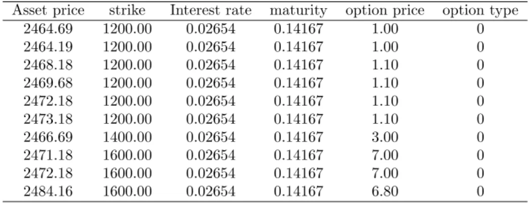
We use the dataset of DAX options on 25th February 2003 to illustrate the IV changes with strike and maturity, table 2.1 is a sample of the data:
Asset price strike Interest rate maturity option price option type
2464.69 1200.00 0.02654 0.14167 1.00 0
2464.19 1200.00 0.02654 0.14167 1.00 0
2468.18 1200.00 0.02654 0.14167 1.10 0
2469.68 1200.00 0.02654 0.14167 1.10 0
2472.18 1200.00 0.02654 0.14167 1.10 0
2473.18 1200.00 0.02654 0.14167 1.10 0
2466.69 1400.00 0.02654 0.14167 3.00 0
2471.18 1600.00 0.02654 0.14167 7.00 0
2472.18 1600.00 0.02654 0.14167 7.00 0
2484.16 1600.00 0.02654 0.14167 6.80 0
Table 2.1: DAX option on 25th Feb, 2003
For convenience, we employ time to maturity τ def= T −t, and the so called future moneyness: κf
def= K/Ft, whereFt=e(r−δ)τSt, is the forward price of stock at time t. We call the options with κ = 1 At The Money(ATM) option. Options close to ATM are usually traded with high frequency. The ATM options are most liquid and
therefore are most available for empirical research.
Fengler (2004) concludes some static stylized facts of IVS observed on different capital market.
(1) The smile is very pronounced for short time to maturity and becomes more and more shallow for longer time to maturities.
(2) The smile function achieves its minimum in the neighborhood of ATM to near OTM call (κ >1) option.
(3) OTM put (κ <1) regions display higher levels of IV than OTM call region.
(4) The volatility of IV is biggest for short maturity options and monotonically decline with time to maturity.
2.2 Calculation of the Implied Volatility
Regardless of the invalid constant volatility assumption of the Black-Scholes model, in practice, the implied volatility can be obtained by inverting the Black-Scholes formula given the market price of the option.
In light of Black-Scholes European call option formula 1.1, we can get ˆ
σ:CBS(St, t, K, T,ˆσ)−C˜t= 0
As we have already observed the evidently curvature shape of the IV σ across the strike K and not so evidently across maturity, it can be described as a function of time, strike prices and expiry days toR+, and if the fixed datat is given, we have :
ˆ
σ: (t, K, T)→ σˆt(K, T)
And this function of the IVσis called implied volatility surface.
Using moneynessκf def= K/Ft, the function of IVσon given datetcan be transformed as:
ˆ
σt(K, T)→ σˆt(κ, τ)
We use a European call as the example to get the volatilityσ. and the implied volatility of a European put on same underlying with same strike and maturity can be deduced from the ”put-call parity”:
Ct−Pt=St−Ke−rτ
The implied Black-Scholes volatility can be determined uniquely from traded option prices because of the monotonicity of the Black-Scholes formula in the volatility para- meter:
∂St
∂σt
>0
The Newton-Raphson algorithm provides a numerical way to invert the Black-Scholes formula in order to recoverσfrom the market prices of the option. XploRe provides a quantlet for this calculation (H¨ardle, Kleinow and Stahl (2002)), the usage of XploRe see H¨ardle, Klinke and M¨uller (2000)
y = ImplVola(x {, IVmethod})
calculates the implied volatility using either the method of bisections or the default Newton-Raphson method, the default method is Newton- Raphson method
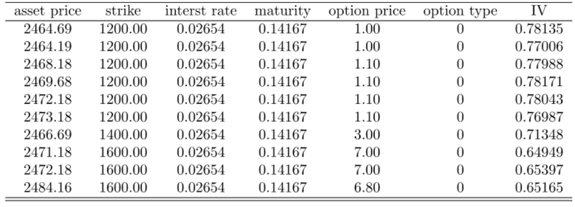
Table 2.2 provides the IV calculated by the quantlet. The data is from DAX options in 25th February 2003. Figure 2.1 plots volatility with strike and moneyness respectively.
asset price strike interst rate maturity option price option type IV
2464.69 1200.00 0.02654 0.14167 1.00 0 0.78135
2464.19 1200.00 0.02654 0.14167 1.00 0 0.77006
2468.18 1200.00 0.02654 0.14167 1.10 0 0.77988
2469.68 1200.00 0.02654 0.14167 1.10 0 0.78171
2472.18 1200.00 0.02654 0.14167 1.10 0 0.78043
2473.18 1200.00 0.02654 0.14167 1.10 0 0.76987
2466.69 1400.00 0.02654 0.14167 3.00 0 0.71348
2471.18 1600.00 0.02654 0.14167 7.00 0 0.64949
2472.18 1600.00 0.02654 0.14167 7.00 0 0.65397
2484.16 1600.00 0.02654 0.14167 6.80 0 0.65165
Table 2.2: IV of DAX option on 022503
ivsmile.xpl
2.3 State Price Density
State price density(SPD) is a fundamental concept in arbitrage pricing theory. The state price density can be understood as the probability density function of underlying
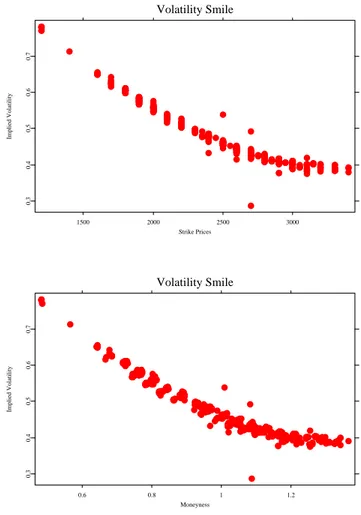
Volatility Smile
1500 2000 2500 3000
Strike Prices
0.30.40.50.60.7
Implied Volatility
Volatility Smile
0.6 0.8 1 1.2
Moneyness
0.30.40.50.60.7
Implied Volatility
Figure 2.1: DAX option on 25th Feb, 2003, τ = 0.14167. Top panel: IV VS strike;
bottom: IV vs moneyness
ivsmile.xpl
asset price, under which the current price of each security is equal to the present value of the discounted expected value of its future payoffs given a risk-free interest rate.
Recall that the Black-Scholes European call option formula is:
CBS(St, t, K, T, σ, r, δ) =e−δτStΦ(d1)−e−rτKΦ(d2), (2.1)
where St is the price of underlying asset at time t,δ is the expected dividends paid over the option’s life,K is the option’s strike price,τ is the time to maturity,ris the risk-free interest rate,
d1= ln(SKt) + (r−δ+12σ2)τ σ√
τ d2=d1−σ√
τ
The price of a european call is the present value of the discounted expected value of its future payoffs given the pdf of underlying asset pricef(St). It can be described as:
Ct(K, T) =e−r(τ) Z ∞
0
(St−K)+f(St)d(St) (2.2) From the definition of SPD, the pdf of underlying asset price f(St) is just SPD. Re- define it as φ(K, T|St, t), deduced from 2.2, SPD is the discounted second derivative of call option price with respect to the strike price:
φ(K, T|St, t) =er(τ)∂2Ct(K, t)
∂K2 (2.3)
The probability that the stock arrived at level K∈[K1, K2] at date T, given that the stock is at levelStint, is computed by:
Q(ST ∈[K1, K2]) = Z K2
K1
φ(K, T|St, t)dK. (2.4) The formula of the second derivative of call option price with respect to the strike price is:
∂2Ct(K, t)
∂K2 =e−r(τ)ϕ(d2) σ√
τ K = e−δ(τ)Stϕ(d1) σ√
τ K2 (2.5)
which yields the specific B-S transition density as:
φ(K, T|St, t) = ϕ(d2) σ√
τ K (2.6)
which is a log-normal pdf in K. It is proved that this log-normal pdf can be written as:
lnST ∼N(lnSt+ (r−δ−1
2σ2)τ, σ2τ) (2.7)
Whereσis a constant. The proof can be seen in Fengler (2004).
2.4 SPD estimation based on IV smile
The motivation for calculating the SPD given IV smile is to insert the IV as a function of strike or moneyness into the B-S call option price formula, and calculate the second derivative of call oprion price with respect to the strike price. Two different method will be introduced here, one is to estimate IV as a function of strike, the other is calculated in moneyness.
Recall that the SPD is the discounted second derivative of call oprion price with respect to the strike price:
φ(K, T|St, t) =er(τ)∂2Ct(K, t)
∂K2 (2.8)
When strike is an explicit function of volatility, the approach to calculate the SPD is discussed in Drescher (2003). It can be derived as below.
First, we need to prove that following relationship always holds:
Ftϕ(d1) =Kϕ(d2) (2.9)
The right hand side can be presented in an alternative way:
Kϕ(d2) = Kϕ(d1−σ√ τ)
= K
√2πexp[−(d1−σ√ τ)2
2 ]
= K
√2πexp[−(d21−2d1σ√
τ+σ2τ)
2 ]
= K
√2πexp[−d21
2 ] exp[d1σ√
τ−σ2τ 2 ]
= Kϕ(d1) exp[d1σ√
τ−σ2τ
2 ] (2.10)
The exponential part of the right hand side is given as:
d1σ√
τ−σ2τ
2 = lnSKt + (r+σ22)τ σ√
τ σ√
τ−σ2τ 2
= lnSt
K + (r+σ2
2 )τ−σ2τ 2
= lnSt
K +rτ (2.11)
Substitute this equation in to the exponent and get:
Kϕ(d2) = Kϕ(d1) exp[lnSt
K +rτ]
= Sterτϕ(d1)
= Ftϕ(d1)
Based on this equation, the Black-Scholes formula for European call option can be rewritten as:
Ct(K, t) =e−rτ[FtΦ(d1)−KΦ(d1−σ√
τ)] (2.12)
Under the assumption that the volatility is a function ofK, the first derivative of the call option price with respect to strike is:
∂Ct(K, t)
∂K = e−rτ[Ftϕ(d1)∂d1
∂K −Φ(d1−σ√
τ)−Kϕ(d1−σ√ τ)(∂d1
∂K − ∂σ
∂K
√τ)]
= e−rτ[Ftϕ(d1)∂d1
∂K −Φ(d2)−Kϕ(d2)∂d1
∂K +Kϕ(d2)∂σ
∂K
√τ]
= e−rτ[∂d1
∂K{Ftϕ(d1)−Kϕ(d2)} −Φ(d2) +Kϕ(d2)∂σ
∂K
√τ]
= e−rτ[−Φ(d2) +Kϕ(d2)∂σ
∂K
√τ] (2.13)
Differentiate the equation 2.13 again with respecct to strike K:
∂2Ct(K, t)
∂K2 erτ = −ϕ(d2)∂d2
∂K +√
τ[{ϕ(d2) +K∂ϕ(d2)
∂d2
∂d2
∂K}∂σ
∂K +Kϕ(d2)∂2σ
∂K2]
= ϕ(d2)[−∂d2
∂K +√ τ ∂σ
∂K −√
τ Kd2∂σ
∂K
∂d2
∂K +√
τ K ∂2σ
∂K2] (2.14) where followng relationship is used:
∂ϕ(d2)
∂d2
= ∂
∂d2
( 1
√
2πexp[−d22 2 ])
= −d2ϕ(d2) (2.15)
And further ∂d∂K2 can be substituted as:
∂d2
∂K = ∂
∂K(lnSt−lnK+rτ−σ22τ σ√
τ ]
= σ√
τ[−K1 −τ σ∂K∂σ]−√
τ∂K∂σ[lnSt−lnK+rτ−σ22τ] σ2τ
= − 1
Kσ√ τ −√
τ∂σ
∂K −d2 σ
σ
K (2.16)
Reorder and combine the above terms together we can achieve the result:
∂2Ct(K, t)
∂K2 =e−rτϕ(d2)[ 1 Kσ√
τ + (2d1 σ )∂σ
∂K + (d1d2K√ τ σ )(∂σ
∂K)2+ (K√ τ)∂2σ
∂K2(2.17)] with:
σ=σ(K) SPD can be calculated with:
φ(K, T|St, t) =ϕ(d2)[ 1 Kσ√
τ + (2d1
σ )∂σ
∂K + (d1d2K√ τ σ )(∂σ
∂K)2+ (K√ τ)∂2σ
∂K2](2.18)
From equation 2.18 we can get the spd equation with the measure of monyness. We always have Ft=e(r−δ)(τ)St, κf =K/Ft
∂σ(K)
∂K = ∂σ(κf) κf
1 Ft
(2.19)
∂2σ(K)
∂K2 = ∂2σ(κf) κ2f
1
Ft2 (2.20)
Insert 2.19 and 2.20 into 2.18, SPD can be computed with:
φ(κf, T|St, t) = ϕ(d2)[ 1 κfFtσ√
τ + (2d1 σ )∂σ
∂κf
1 Ft
+ (d1d2κfFt√ τ σ )(∂σ
∂κf
)2 1 Ft2 + (κfFt√
τ)∂2σ
∂κ2f 1
Ft2] (2.21)
with:
σ=σ(κf)
The accompanied quantletspdcalandspdcalmis introduced in the next subsection.
2.5 The Quantlet spdcal and spdcalm
fstar= spdcal(k, sig, sig1, sig2, s, r, tau) Calculate the empirical state-price density
The quantlet spdcal uses function 2.18 to compute the SPD. The analytic formula uses an estimate of the volatility smile and its first and second derivative to calculate the State price density, This method can only be applied to European options (due to the assumptions).
The quantletspdcalhas the following input parameters.
k-N×1 vector of strike prices
sig-N×1 vector of points of the estimated volatility
sig1 -N×1 vector of points of the first derivative of the volatility smile (with respect to strike price)
sig2 - N ×1 vector of points of the second derivative of the volatility smile (with respect to strike price)
s-N×1vector, underlying spot price corrected for dividends r -N×1 vector, risk-free interest rate
tau -N×1 vector, time to maturity Output Parameter
fstar-N×1 vector of state-price density
fstar= spdcalm(m, sig, sig1, sig2, s, r, tau)
Calculate the empirical state-price density with moneyness measure
The quantlet uses function 2.21 to compute the SPD. The analytic formula uses an estimate of the volatility smile with respect to moneyness and its first two derivatives to calculate the SPD, This method can only be applied to European options (due to the assumptions).
The quantletspdcalhas the following input parameters.
m-N×1 vector of moneyness
sig-N×1 vector of points of the estimated volatility
sig1 -N×1 vector of points of the first derivative of the volatility smile (with respect to strike price)
sig2 - N ×1 vector of points of the second derivative of the volatility smile (with respect to strike price)
s-N×1vector, underlying spot price corrected for dividends r -N×1 vector, risk-free interest rate
tau -N×1 vector, time to maturity Output Parameter
fstar-N×1 vector of state-price density
2.6 Arbitrage Free Constraint
A lot of recent researches have contributed to estimation of no-arbitrage SPD. The practical way to estimate SPD might be roughly classified into 2 groups. One is the direct approach based on the observation of option price, to fit the observations of option price to the theoretical option prices, and derive the prespecified SPD from the second derivatives of option price with respect to strike. H¨ardle and Hl´avka (2005) have used non parametric method to estimate SPD from DAX option price data with this direct approach. The other is the indirect approach based on volatility smile. First recover volatility smile into the call price and then get SPD. This indirect method have been discussed in section 2.4, it was first introduced by Shimko (1993).
No matter what method has been employed, the difficulty of estimation is the impo- sition of arbitrage-free constraint. The call price function, according to H¨ardle and Hl´avka (2005), has following no-arbitrage constraint:
1. it is positive
2. it is decreasing in K 3. it is convex
4. its second derivative exists and it is a density (i.e.,nonnegative and it integrates to one)
The constraint 1 and 2 is obvious, the constraint 4 is derived from general property of density function. The constraint 3 is deduced from arbitrage free condition require- ments, see 7.2.1.
The shape constraint of European call price can be ”translated” to the shape constraint of volatility smile. But this translation process is easy to explain in theory but bitter in practice. Below we list some general shape constraint for volatility smile through the strike direction (not restricted to no-arbitrage constraint ).
1. Estimated volatility should be positive.
ˆ
σ≥0 (2.22)
2. There exists the lower bound and upper bound of the first derivative of volatility with respect to strikeK. This can be expressed as:
− Φ(−d1)
√τ Kϕ(d1) ≤ ∂σˆ
∂κf
≤ Φ(−d2)
√τ Kϕ(d2) (2.23) UsingFt=e(r−δ)(τ)St, κf =K/Ft, this can be expressed in terms of moneyness measure:
− Φ(−d1)
√τ κfϕ(d1) ≤ ∂σˆ
∂κf
≤ Φ(−d2)
√τ κfϕ(d2) (2.24)
3. the right hand side of 2.18 is nonnegative and integrates to one, we can obtain 1
Kσ√ τ +
2d1
σ ∂σ
∂K + (d1d2K√ τ σ )(∂σ
∂K)2+ (K√ τ)∂2σ
∂K2 ≥0 (2.25) Z
K
Φ(K, T|St, t)dK = 1 (2.26)
When K is on the limit interval [Kl, Kh] Z Kh
Kl
Φ(K, T|St, t)dK ≤1 (2.27)
Constraint 2 can be proved, see Appendix 7.2.2. Constraint 3 is translated from the constraint 4 of call price function.
Polynomial Estimator
There are several studies fitted parametric volatility functions to observed implied volatilities. Shimko (1993), Tompkins (1999), An´e and German (1999) and An´e and German (1999) are among this group. They usually employ quadratic specifications to model the IV function along the strike profile. These parametric approaches are not able to capture the prominent feature of IVS patterns, and hence the estimates maybe biased. Others are focus on non-and semiparametric smoothing approaches to estimate IVS. A¨ıt-Sahalia and Luo (1998), Rosenberg (2000), Cont et al. (2002) and Fengler (2004) applied a Nadaraya-Watson estimator to the IVS, and higher order local polynomial smoothing of the IVS is used in Rookey (1997). Below we’ll give a short introduction to this non-parametric method.
For simplicity, consider the univariate model
Y =m(X) +ε (3.1)
with the unknown regression functionm. The explanatory variableXand the response variable Y take values inR, have the joint pdff(x, y) and are independent ofε. The errorεhas the propertiesE(ε|x) = 0 andE(ε2|x) =σ2(x).
Taking the conditionalexpectation of 3.1 yields
E(Y|X =x) =m(x) (3.2)
which says that the unknown regression function is the conditional expectation function ofY givenX=x. Using the definition of the conditional expectation 3.2 can be written as:
m(x) =E(Y|X=x) =
R yf(x, y)dy
fx(x) , (3.3)
where fx(x) denotes the marginal pdf. Representation 3.3 shows that the regression function m can be estimated via the kernel density estimates of the joint and the marginal density.
In the book of H¨ardle, M¨uller, Sperlich and Werwatz (2004) the Nadaraya-Watson estimator is introduced:
ˆ
m(x) = n−1Pn
i=1Kh(x−xi)yi n−1Pn
i=1Kh(x−xi) (3.4)
Rewriting above formula as ˆ
m(x) = 1 n
n
X
i=1
Kh(x−xi) n−1Pn
j=1Kh(x−xj)yi= 1 n
n
X
i=1
ωi,n(x)yi (3.5) This formula indicates that the Nadaraya-Watson estimator can be seen as a weighted (local) average of the response variables with weights:
ωi,n(x)def= Kh(x−xi) n−1Pn
j=1Kh(x−xj) (3.6)
Here Kh(•) denotes univariate Kernel function, Quartic kernel or Gaussian kernel are the most widely used kernels:
Quartic(Biweight)kernel
Ku= 15
16(1−u2)2I(|u| ≤1) (3.7) Gaussian kernel
Ku= 1
√2πexp(−1
2u2) (3.8)
The Nadaraya-Watson estimator can be seen as a special case of a larger family of Local smoothing estimators. One generalization is Local PolynomialRegression.
minβ n
X
i=1
{(Yi−β0−β1(Xi−x)−...−βp(Xi−x)p)}2Kh(x−Xi) (3.9) where β denotes the coefficients vectorβ = (β0, β1, ..., βp)>
we can computeβ by using weighted least squares estimator with weightsKh(xi−x), it has been studied extensively by Fan and Gijbels (1996).
We introduce the following matrix notation:
X=
1 x−x1 (x−x1)2 . . . (x−x1)p 1 x−x2 (x−x2)2 . . . (x−x2)p ... ... ... . .. ... 1 x−xn (x−xn)2 . . . (x−xn)p
, (3.10)
andY = (y1, ..., yn)>, and the weight matrix:
X=
Kh(x−x1) 0 . . . 0 0 Kh(x−x2) . . . 0
... ... . .. ...
0 0 . . . Kh(x−xn)
, (3.11)
Then we can write the solution of 3.9 in the usual LSE formulation as:
βˆx= (X>W X)−1X>W Y (3.12) For p = 0,βˆ reduces to β0, we get Nadaraya-Watson estimator. And the order p is usually taken to be one (local linear) or three (local cubic regression). Nadaraya- Watson regression corresponds to a local constant least squares fit.
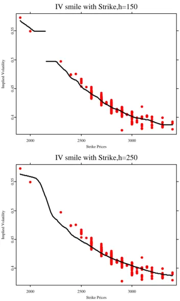
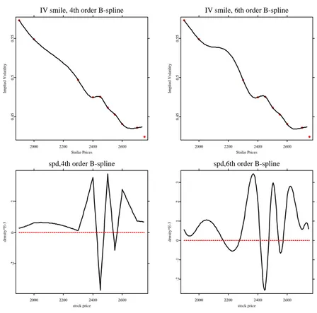
We plot IV smile by using Nadaraya-Watson regression figure 3.1, 3.2 and second order local polynomial regression figure 3.3, 3.4. In Nadaraya-Watson case, when the bandwidth is small, the estimator failed to generate a continuous function; if we enlarge the bandwidth, the large bias appears and the curve can’t fit to the data, especially in the region where the observations are sparse. The local polynomial regression approach has at least 2 superiorities over Nadaraya-Watson estimator. The first is that local linear estimator improved the estimates in boundary regions. When we use Nadaraya- Watson approach, possibly some of the points are used more than ones to estimate the curve near the boundary. This problem is improved since Local polynomial imposes a higher degree polynomial here. The second is that if we use local polynomial approach, it will be easier to estimate the derivatives of function m(•). This advantage is very useful in estimating IV based state price density, since the estimation of SPD requires the estimation of IV and it’s first two derivatives. We also plot the estimated SPD in figure 3.3, 3.4.
IV smile with Strike,h=150
2000 2500 3000
Strike Prices
0.40.450.50.55
Implied Volatility
IV smile with Strike,h=250
2000 2500 3000
Strike Prices
0.40.450.50.55
Implied Volatility
Figure 3.1: IV smile with strike, DAX call option,02-25-03,τ= 0.14167. Upper panel:
Bandwidth=150, lower panel: Bandwidth=250. Nadaraya-Watson estima-
tor is used. spdcalnw.xpl
IV smile with Moneyness, h=0.05
0.8 0.9 1 1.1 1.2 1.3
moneyness
0.40.450.50.55
Implied Volatility
IV smile with Moneyness, h=0.1
0.8 0.9 1 1.1 1.2 1.3
moneyness
0.40.450.50.55
Implied Volatility
Figure 3.2: IV smile with moneyness, DAX call option,02-25-03, τ = 0.14167. Upper panel: Bandwidth=0.05, lower panel: Bandwidth=0.1. Nadaraya-Watson
estimator is used. spdcalnwm.xpl
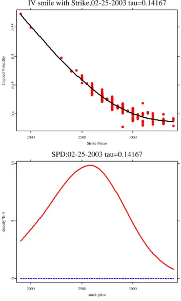
IV smile with Strike,02-25-2003 tau=0.14167
2000 2500 3000
Strike Prices
0.40.450.50.55
Implied Volatility
SPD:02-25-2003 tau=0.14167
2000 2500 3000
stock price
0510
density*E-4
Figure 3.3: DAX call option,02-25-03,τ= 0.14167. Upper panel: IV smile with strike, right panel: SPD. Bandwidthh= 700, the second order local polynomials
is used. spdcallp.xpl
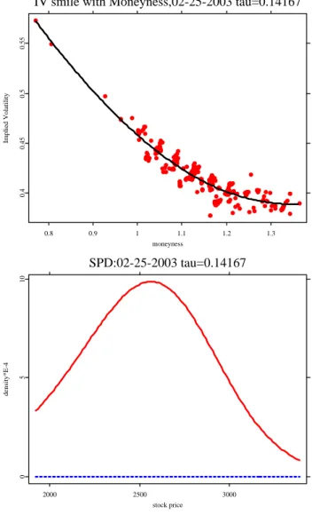
IV smile with Moneyness,02-25-2003 tau=0.14167
0.8 0.9 1 1.1 1.2 1.3
moneyness
0.40.450.50.55
Implied Volatility
SPD:02-25-2003 tau=0.14167
2000 2500 3000
stock price
0510
density*E-4
Figure 3.4: DAX call option,02-25-03,τ= 0.14167. Upper panel: IV smile with strike, right panel: SPD. bandwidthh= 0.4, the second order local polynomials
is used. spdcallpm.xpl
Approach
4.1 Basic Setup
In every working day, options are traded frequently in financial market. For each transaction, we can calculate one implied volatility. If we collect the data time by time and day by day, we can recover implied volatility to a function of strike K and maturity τ. Due to this attribute we may understand IV as functional data in that each observation is a real function of underlying variables. We can find some other examples of functional data in many fields, such as human growth, which is a function of time or age; weather data is another example since its dependence on other observations such as temperature and humidity. The basis function approach for representing functional data as smooth functions, provides us more flexible smoothing techniques for estimation out of discretely observed data.
Formally, a sample of multivariate data X = {X1, ..., Xn} is described as (n×p) matrix containing nobservations ofp-dimensional row vectors ofp(one dimensional) random variables (2 ≤ p <∞). It is the measurable mapping (Ω,A,P)→ (Rp,B), where (Ω,A,P) is a probability space, Ω is the set of all elementary events, A is a sigma algebra of subsets of Ω, and P is a probability measure defined onA. Rp is a p-dimensional vector space,Bis a sigma algebra onRp.
In the case of functional data, X consists of random functions, we denote the ith observations as Xi(t), i= 1, ..., n of some argument t. It is the measurable mapping (Ω,A,P)→(H,BH), whereHis the space of functions.
We denote the i-th observation as Xi(t), i = 1, ..., n of some argument t. It will be assumed that the functions are observed on a finite interval J= [tL, tU]∈R, wheretl and tU denotes the lower and upper bound, respectively. Ramsay and Dalzell (1991) introduce the name functional data analysis (FDA) and give the following definition:
Functional data:
A sample X = {X1, ..., Xn} is called functional data where thei-th observation is a real functionXi(t), t∈J, i= 1, ..., n, and hence, eachXi(t) is a point in some function spaceH.
A single functional observation, which means a single observed function, is called a replication. Functional data in turn is a random sample of replications. In this paper, we will use one-day data, fix the maturity and focus on estimating IV function of strike by smoothing techniques from functional data analysis. In our case, we have only one replication. More advanced method for functional data can be found in Ramsay and Silverman (1997)
4.2 The Basis Function Approach
We want to present functional data as smooth functions of some continuous parame- ters. Generally we have no idea in advance how these curves look like, how complex they will be and what certain characteristics they may have, typically we will assume just some degree of smoothness. For this reason flexibility is the key issue we demand for estimation. To solve this problem we need some mathematical ”machinery”, with which we can do any computation that is needed to fit the data quickly and flexibility.
The core idea is to replace the vector of inputs twith additional variables, which are transformations of t, and then use linear models in this new space of derived input features. See Hastie, Tibshirani and Jerome (2001).
For simplicity, consider the following univariate model:
Y =X(t) +ε (4.1)
Our approach is to minimize the penalized residual sum of squares
minX∈HK[{Y −X(t)}>{Y −X(t)}+λP EN(X(t))] (4.2) where HK is the Hilbert space of real function K. λ is a smoothing parameter, P EN(X(t)) is the penalty operator. We will discuss the penalized regression in more detail in Section 4.4.
According to Wahba (1990), the solution to 4.2 and even to a more general class of penalized regression problems has the form of finite-dimensional linear combination
Xˆ(t) =
K
X
k=1
ckφk(t), ck ∈R;K <∞ (4.3) where φk(t) is a real-valued function and following Hastie et al. (2001), it is referred to as basis function. This approach can be seen as a particular linear regression model
with each variables being some basis functions. Once these functionsφk(t) have been defined, we can fit them to classical linear model as before. And this approach in estimation X(t) with 4.3 is called ”Basis function Approach”.
4.3 B-spline Bases
A wide range of basis functionφ(t) can be applied in this approach, the most popular are Fourier Bases, Polynomial bases and B-spline bases. B-spline will be introduced here since its flexibility in representing X(t). If there exists a space of piecewise polynomials, B-spline is a basis of certain subspace of that space .
We divide the intervalJ = [tL, tU] into several continuous intervals and representX(t) by separate polynomial in each interval. X(t) is a piecewise polynomial function.
Follow the definition of de Boor (1978), the piecewise polynomial can be described as below:
Definition 1 (piecewise polynomial)Divide the intervalJ = [tL, tU]intomsubin- tervals by a strictly increasing sequence of pointstL=ξ1< ξ2< ... < ξm< ξm+1=tU. The pointsξi are called breakpoints. LetKbe a positive integer. Then the correspond- ing piecewise polynomial function X(t)of order K is defined by
X(t)def= p(t) =
K−1
X
j=0
cjtjI{x∈[ξi, ξi+ 1]}, i= 1, ..., m (4.4)
If we restrict that the piecewise function, some times their higher order derivatives to be continuous in each breakpoint, we will obtain the polynomial splines. de Boor (1978)also define the polynomial splines as below:
Definition 2(polynomial spline) Let K > 0 be an integer indicating the order of piecewise polynomials, ξ = ξim+1
i=1 be a given breakpoint sequence with tL =ξ1 <
ξ2 < ... < ξm < ξm+1 =tU, the vector ν ={νi}mi=2 counts the number of continuity conditions at each interior breakpoint. If νi = K −1 for all i = 2, ..., m then the piecewise polynomial function Xi(t)is called polynomial spline of order K.
B-splines has been defined as a divided difference of the truncated power basis. And it is formally defined as:
Definition 3(B-splines)
θl(t) =Bl,K(t), l= 1, . . . , m+k−2 (4.5) whereBl,K isl-th B-Spline of order K, for the non-decreasing sequence of knots{τi}mi=1
defined by following recursion scheme:
Bi,1(t) =
1, fort∈[τi, τi+1] 0, otherwise Bi,k(t) = t−τi
τi+k−1−τi
Bi,k−1(t) + τi+k−t τi+k−τi+1
Bi+1,k−1(t) fori= 1, . . . , m+k,k= 0, . . . , K.
The number of the basis function will uniquely be defined by the B-spline order and the number of knots, whilenbasis=nknots+norder−2. Flexibility is one advantage of the B-spline basis and its also relatively easy to evaluate the basis functions and their derivatives. XploRe quantletBsplineevalgdcan be used for this approach.
4.4 Estimation of Coefficients
Consider the basis function approach f(x) =
K
X
k=0
ckφk(x) (4.6)
Estimate ck by the observed data (xj, yj), j= 1, ..., n
Y = ΦC+ε (4.7)
where Y = (y1, ...yn)>,{Φ}k =φk(x), C= (c1, ..., cK)>, ε= (ε1, ...εn)>. The Generalized Least Squares (GLS) estimation of coefficient c is:
Cˆ= (Φ>Φ)−1Φ>Y (4.8)
Using 4.7 we leave the degree of smothness just by the order of B-spline. It is merely interpolating the data, without exploiting some structure noises might present in the data. We may use some additional information of function f(x), and add a roughness penalty to ’penalize’ the non smoothness.
Due to the insight of Ramsay (1997), it is the smoothness of the process generating functional data that differentiates this type of data from more classical multivariate observations. This smoothness ensures that the information in the derivatives of func- tions can be used in a reasonable way. We can make use of the fact that the curvature of the curve f(x) increases with||f00(x)||, and get the total curvature as measure of roughness penalty
P EN2(f) = Z
J
{D2f(s)}2ds=||D2f||2 (4.9)
When using basis expansionf(X) = ΦC, the penalty term can be written as
P EN2(f) =C>RC (4.10)
where {R}ij =R
J{D2φi(s)}{D2φj(s)}ds=hD2φi, D2φji
Now we can match the observation with the smooth function by solving the minimiza- tion of penalized residual sum of squares function:
fˆλ=argminfP EN SSEλ(f|y) (4.11)
P EN SSEλ(f|y) = (Y −ΦC)>(Y −ΦC) +λC>RC (4.12) The parameter λcontrols the weight given to the stabilizer in the minimization. The higher theλis, the more weight is given to||f00(x)||, and the smoother is the estimator.
λcan be chosen by Cross validation method.
The linear differential operator (LDO) can be used as a more generalized roughness Penalty.
Lf(x) =ω0(x) +ω1(x)Df(x) +...+ωm−1Dm−1f(x) +Dmf(x) (4.13) The Generalized penalized residual sum of squares function:
P EN SSEλ(X|y) = (Y −ΦC)>(Y −ΦC) +λ||Lf||2 (4.14) where ||Lf||2=C>RC, with{R}ij=R
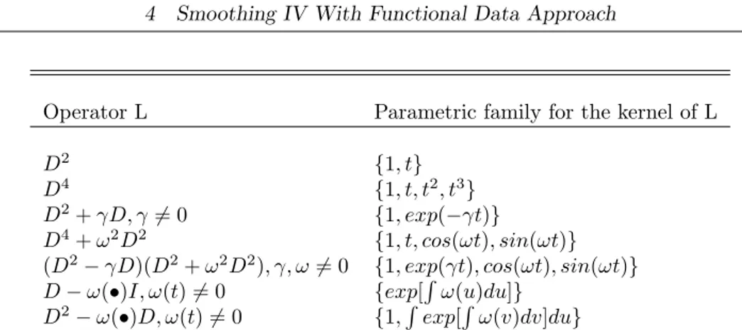
J{Dmφi(s)}{Dmφj(s)}ds=hDmφi, Dmφji In practice, since many models are based on scientifical or phisical models, there is a general idea of the order and coefficients of LDO. Sometimes, we may be able to surmise the shape of smoothed curve, thus we can be motivated to choose special LDOs to incorporate this shape speculation. There are links between some linear differential operator and bases for the corresponding parameter families. Heckman and Ramsay (2000) provides table 4.1 for some examples of differential operators and the bases for the corresponding parametric families
4.5 Choice of the Smoothing Parameter
Technically, two possible approaches can be applied to choose the smoothing parameter λ. As discussed by Green and Silverman (1994). The first approach is to choose the smoothing parameter λ subjectively. With differentλ, different features of the data that arise from different ”scales” can be explored, and the one parameter value which
”looks best” might be chosen. The second approach is to choose λ automatically
Operator L Parametric family for the kernel of L
D2 {1, t}
D4 {1, t, t2, t3} D2+γD, γ6= 0 {1, exp(−γt)}
D4+ω2D2 {1, t, cos(ωt), sin(ωt)}
(D2−γD)(D2+ω2D2), γ, ω6= 0 {1, exp(γt), cos(ωt), sin(ωt)}
D−ω(•)I, ω(t)6= 0 {exp[R
ω(u)du]}
D2−ω(•)D, ω(t)6= 0 {1,R exp[R
ω(v)dv]du}
Table 4.1: Examples of differential operators and the bases for the corresponding para- metric families.
based on the data set its self, one popular method of which is cross validation. In many cases these two approaches can be combined, and an automatic choice can be used as a starting point for subsequent subjective adjustment.
Cross-validation seems to be the most frequently used methods for choosing the smooth- ing parameter. The main idea of this method is to split the data set into two parts, the ”learning ” sample and the ”validation” sample. First, fit the data to the model by using learning sample then assess the fit to the validation sample, and finally choose theλvalue by minimizing some error criterion. We can split the data by the ” leave- one-out” rule. This method is to leavei-th observation out , and the functionXi(t) is predicted from other functions in the data set.
Following Ramsay and Silverman (2002), let m−iλ (ti) denote the smoothed sample mean calculated with smoothing parameter λ from all observations except ti. As a measure of global discrepancy compute the integrated squared error(ISE)
ISE{m−iλ (ti)}= Z
J
{m−iλ (ti)−yi}2dt, (4.15) to see how well m−iλ (ti) predicts m−iλ (ti). The cross-validation score CV(λ) is com- puted by summing up the square errors over all n observations.
CV(λ) =
n
X
i=1
{m−iλ (ti)−yi}2dt. (4.16) The smaller the value of CV(λ), the better the performance of λ as measured by cross-validation score. Hence, minimizing 4.16 with respect to λ gives the optimal smoothing parameter.
Since cross-validation is very time consuming, and leads to under-smoothing the data so often, the generalized cross-validation criterion has been introduced by Eubank (1988). Here, the value of λis chosen to minimize
GCV(λ) = nSSE(λ)
(n−dfλ)2 = n
n−dfλσˆ2(λ) (4.17) where SSE(λ) ={Y −Φ(t) ˆC}>W{Y −Φ(t) ˆC} and ˆσ2(λ) =SSE(λ)/(n−dfλ). W is the weight matrix. dfλ is the effective number of parameters of degrees of freedom that ˆX(t) = Φ(t) ˆC uses in estimatingX(t). Heckman and Ramsay (2000) define:
dfλ=tr(SΦ,λ) + number of estimated parameters (4.18) whereSΦ,λis the smoothing matrix as defined in the last section. Usually, the numera- tor of GCV is small (i.e.,Φ(t) ˆCis close to interpolating the data) when the denominator is small (when dfλ is close to n). Thus minimizing GCV means fitting the data well with few parameters, see Heckman and Ramsay (2000).
The XploRe quantlet bfacvand bfagcvwill be introduced in the section 4.6. These quantlets are used to calculate the CV or GCV of different smoothing parameter λ.
4.6 The Quantlet Bfacv and Bfagcv
cvl,L= bfagcv(y,argval,fdbasis{,Lfd{,W{,lambda}}})
Calculate the generalized cross-validation score for smoothing parameter lambda
This quantlet uses 4.16 to compute the GCV score. The syntax of the quantlet is:
cvl,L= bfagcv(y,argval,fdbasis{,Lfd{,W{,lambda}}}) with input parameters:
y- a vector of (observed) functional values used to compute the functional data object.
argvals- vector matrix of argument values.
basisfd- an fdbasis object
Lfd - Identifies the penalty term. This can be a scalar (≥1) containing the order of derivative to penalize, or an LDO object if an LDO with variable coefficients. When applying an LDO with constant coefficients, Lfd is a (r×2) matrix, where the first
column contains the coefficients, the second one the orders of derivatives. The default value is Lfd = 2.
W- Weight matrix. The default value is the identity matrix.
lambda - Parameter for roughness penalty smoothing. If lambda is not specified it will be estimated by the data.
When lambda is not given, it will be calculated by λ= 10−4tr{φ(t)>Φ(t)}
trR (4.19)
Lambda will also be returned as the output parameter L.
gcv,L= bfagcv(y,argval,fdbasis{,Lfd{,W{,lambda}}})
Calculate the generalized cross-validation score for smoothing parameter lambda
This quantlet uses 4.17 to compute the GCV score. The syntax of the quantlet is:
gcv,L= bfagcv(y,argval,fdbasis{,Lfd{,W{,lambda}}}) with input parameters:
y-p1×p2×p3 array of (observed) functional values used to compute the functional data object. p1 is the number of observed values per replication,p2 is the number of replications,p3 is the number of variables.
argvals - (n×m) matrix of argument values, wherem= 1 orm=p2, respectively.
If m= 1 the same arguments are applied to all replications and variables. Otherwise it must hold that m = p2, then each replication is applied to a certain vector of arguments.
basisfd- an fdbasis object
Lfd - Identifies the penalty term. This can be a scalar (≥1) containing the order of derivative to penalize, or an LDO object if an LDO with variable coefficients. When applying an LDO with constant coefficients, Lfd is a (r×2) matrix, where the first column contains the coefficients, the second one the orders of derivatives. The default value is Lfd = 2.
W- Weight matrix. The default value is the identity matrix.
lambda - Parameter for roughness penalty smoothing. If lambda is not specified it will be estimated by the data for each replication separately.
As this quantlet will usedata2fd(see Ulbricht (2004))to estimate the coefficients, the syntax of it is in consistency withdata2fd. The difference is that it does not return an fd object, but the GCV score with respect to smoothing parameter lambda. lambda will also be returned as the output parameter L. When lambda is not given, it will be calculated by 4.19 by using the input parameters y and argvals. If necessary, lambda is computed individually for each replication. If lambda should be zero, then this must be given as input parameter. Note, if the number of basis functions is greater than the number of observations of a single replication, lambda will be estimated by the above formula in any case, even if the corresponding input parameter is set equal to zero.
Otherwise (4.17) could not be used because the outer product of the basis matrices in singular in this case. And the value of the estimated lambda will be output, too.
The input parameter y can be a vector, matrix or three-dimensional array, respectively.
The missing value problem is processed with the same method as indata2fd. When some observations at some arguments are missing just insert NaNs. This is also the case when the number of observations vary between the replications. The algorithm filters out the NaNs. The input parameter argvals cannot contain NaNs, otherwise the getbasismatrix quantlet need to be readjusted in order to handle NaNs. If a functional value is missing for a certain argument, then just give an arbitrary value to the argument. The algorithm will filter out the pair of values in any case. It takes more computation time when NaNs are included in the functional data input because the compiler need to calculate the coefficients for each replication separately, see Ulbricht (2004).
We will use some minimization method such as Brent’s method or Golden section search, to choose optimalλ.
B-splines on Financial Market Data
5.1 Construction of Model
In this chapter, we will compare the estimation results for different value of smoothing parameters, and choose smoothing parameterλby cross validation or generalized cross validation. The algorithm of smoothing IV-Strike function includes following steps:
• Define a sequence of non-decreasing knots. When dealing with strike, we use distinct strike prices as the break points. When using moneyness as argument, we set non-decreasing knots every 5 points of sorted moneyness.
• generate basis matrix Φ on the vector of knots;
• Define the penalty operator;
• Choosing the smoothing parameter;
As we have obtained the smoothing function, now we will use it to get SPD. The algorithm is presented as follow:
• Generate a grid on the range of strike price.
• Using the grid points generated from last step as argument values and insert it into the IV smile function. calculate the estimated volatilities and first deriva- tives as well as second derivatives.
• Using median of stock price asSt, insert the estimated volatilities, first deriva- tives, second derivatives into 2.18, and calculate SPD.