The Discrete Element Method in Archaeoseismological Research –
Two Case Studies in Israel
Inaugural-Dissertation zur
Erlangung des Doktorgrades
der Mathematisch-Naturwissenschaftlichen Fakultät der Universität zu Köln
vorgelegt von
Gregor Schweppe
aus Vreden
Köln 2019
Berichterstatter/Gutachter: Prof. Dr. K.-G. Hinzen
Prof. Dr. M. Melles
Tag der mündllichen Prüfung: 06.06.2019
Für meine Eltern
Christel und Hermann Schweppe
I. Abstract ... i
II. Zusammenfassung ... ii
III. Acknowledgement ... iv
1 Introduction ... 1
1.1 Archaeoseismology ... 3
1.2 Archaeoseismological Research in Israel ... 8
1.3 Two Case Sites in Israel ... 9
1.4 Guidelines of the Thesis ... 12
2 Region of Interest ... 13
2.1 Geographical Overview ... 13
2.2 Geological Overview ... 15
2.3 Tectonic ... 19
2.4 Seismicity ... 20
2.4.1 Intensity ... 20
2.4.2 Magnitude ... 22
2.4.3 Pre-Instrumental Earthquakes ... 23
2.4.4 Instrumental Earthquakes ... 25
3 Laser Scanning ... 27
4 Computer Models ... 31
4.1 Discrete Element Method ... 32
4.2 Model Verification ... 32
4.3 Collision detection ... 34
4.4 Units ... 35
4.5 Damping ... 36
4.6 Discrete Fracture Network ... 36
4.7 Software solutions ... 36
4.7.1 Universal Mechanism ... 37
4.7.2 Unity 3D ... 40
4.7.3 3 Dimensional Distinct Element Code ... 42
5.1 History of the Temple ... 48
5.2 Virtual 3D Model from Laser Scans ... 51
5.3 Creation of Discrete Element Models ... 52
5.3.1 Universal Mechanism ... 53
5.3.2 3 Dimensional Distinct Element Code ... 55
5.3.3 Unity 3D ... 56
5.4 Calculations ... 56
5.4.1 Analytic Ground Motion Signals ... 56
5.4.2 Earthquake Scenarios ... 57
5.5 Results ... 59
5.6 Discussion and Conclusion ... 66
5.7 Further Research ... 67
6 Crusader Fortress Ateret ... 68
6.1 History of the Site ... 69
6.2 Reconstruction of the Original State ... 73
6.3 Model Creation ... 77
6.4 Calculations ... 83
6.5 Results ... 85
6.5.1 First Scenario ... 87
6.5.2 Second Scenario ... 100
6.6 Discussion and Conclusion ... 106
6.7 Further Research ... 109
7 Discussion and Conclusion ... 111
8 Literature ... 112
9 Data and Resources ... 127
A. Appendix Crusader Fortress Ateret ... 128
a. First Scenario ... 128
b. Second Scenario ... 150
Erklärung ... 186
I
I. A BSTRACT
Quantitative methods and particularly computer simulations have become increasingly important in the field of archaeoseismology in recent decades. In this work two approaches to investigate the ground motion history of two specific archaeological sites with computer models based on the discrete element method (DEM) are presented. During the model development, three different software codes are tried out to test which are suited best for these simulations.
Both sites that are in the focus of this work are located in Israel, a country rich on archaeological sites. At the ruin of the Roman Temple of Kedesh the concept of precariously balanced archaeological structures (PBAS) was introduced, in which the presence or absence of a certain ground motion in the past can be estimated. Since the destruction of the temple the ruin was exposed to numerous earthquakes. The goal here was to identify which ground motion would have destroyed the ruin. In 108 simulations with cycloidal pulses as ground motion with major frequencies ranging from 0.3 Hz to 2.0 Hz and PGAs from 1 m/s² to 9 m/s² the response of the ruin was calculated. Additionally, eight earthquake scenarios with two assumed, five historical and one recorded earthquake (ChiChi 1999) were used to test the stability of the ruin. The results of the simulations with the earthquakes show that only the record of the strong ChiChi earthquake would have destroyed the remains of the temple. The concept of PBAS does not only provide information about the current stability of the structure, which may be important in terms of the conservation of the cultural heritage, but also gives information about the parameters of the past earthquakes ground motions.
At the second site a different approach was followed. The ruin of the Crusader Fortress of Tell Ateret sits
directly on the Dead Sea Transform Fault (DSTF); the fortification walls show a significant lateral offset
that is related to movement along the fault line. At this point it is unknown whether the offset is the
consequence of rapid movements during earthquakes or (at least in part) of slow creeping motion along
the fault. In a discrete element (DE) model the original state of the northern fortification wall was
reconstructed. The reconstruction formed the basis for 58 numerical simulations, in which the response of
the model to ground motions were calculated. The simulations covered different movement directions and
slip velocities along the fault line. The results show that a slow creeping movement could be ruled out as
origin for the offset of the fortification walls. Furthermore, the results support the hypothesis that two
coseismic movements displaced the fortification walls and also reveal that most of the slip occurred east
of the fault line. Slip velocities of 3 m/s and 1 m/s could be estimated for the two movements. These can
be assigned to two past earthquakes which occurred on May 20th 1202 and October 30th 1759.
II
II. Z USAMMENFASSUNG
In den letzten Jahrzehnten nahm die Bedeutung von quantitativen Methoden, besonders von Computer- Simulationen in archäoseismologischer Forschung zu. In dieser Arbeit werden für zwei ausgesuchte archäologische Stätte Ansätze zur Untersuchung der Bodenbewegungsgeschichte mit Computer Modellen vorgestellt, die auf der Diskrete-Elemente-Methode (DEM) basieren. Während der Modellentwicklung wurden drei Programmsysteme getestet, um festzustellen, welche am besten für unterschiedliche Fragestellungen geeignet sind.
Beide ausgewählten Stätte liegen in Israel, das reich an archäologischen Hinterlassenschaften ist. Das Konzept der prekär balancierten archäologischen Strukturen (PBAS) wird an der Ruine des Römischen Tempels von Kedesh eingeführt, mit dessen Modell das Vorhandensein oder Fehlen von Bodenbewegungen bestimmter Stärke in der Vergangenheit abgeschätzt werden kann. Seit der Zerstörung des Tempels war die Ruine mehreren Erdbeben ausgesetzt. Das Ziel war es, herauszufinden, welche Bodenbewegung die Ruine zerstört hätte. Dafür wurden 108 Simulationen durchgeführt, bei denen Cycloidal-Pulse mit Frequenzen von 0.3 Hz bis 2.0 Hz und Maximal-Beschleunigungen von 1 m/s² bis 9 m/s² als Bodenbewegungen verwendet wurden. In acht zusätzlichen Simulationen wurden synthetische Seismogramme von zwei angenommenen und fünf historisch belegten Erdbeben in der Levante sowie Messungen des ChiChi Erdbebens 1999 als Bodenbewegung verwendet, um die Stabilität der Ruine zu testen. Die Ergebnisse zeigen, dass nur Bodenbewegungen mit Amplituden ähnlich die des ChiChi Erdbebens die Ruine zerstört hätten, den Simulationen mit den historischen Erdbeben widerstand das Modell der Ruine. Der Ansatz der PBAS erlaubt es nicht nur Grenzen der Bodenbewegungsparameter der historischen Erdbeben anzugehen, sondern auch Aussagen über die momentane Stabilität der Struktur zu machen, welche wichtig für den Erhalt des Kulturerbes sein können.
An der zweiten Stätte wurde ein anderer Ansatz verfolgt. Die Kreuzritter Festung Ateret wurde direkt auf
der Störungslinie der Toten Meer Transformstörung errichtet. Die Festungsmauern zeigen einen lateralen
Versatz der zwischen 2.1 und 1.75 m variiert, der zuvor als Resultat von rein coseismischen Bewegungen
an der Störungslinie interpretiert wurde. Bislang war jedoch unklar, ob nicht zumindest teilweise langsame
(postseismische) Kriechbewegungen entlang der Störungslinie zum Gesamtversatz beigetragen haben, was
einen deutlichen Einfluss auf die Magnitudenbestimmung der Beben hätte. In einem Diskrete-Elemente
(DE) Modell wurde der ursprüngliche Zustand der Ruine vor dem Versatz rekonstruiert. Basierend hierauf
wurden 58 numerische Simulationen durchgeführt, wobei unterschiedliche Versatzgeschwindigkeiten und
unterschiedliche Versatzrichtungen auf beiden Störungsseiten berücksichtigt wurden. Die Ergebnisse
zeigen, dass eine Kriechbewegung als Ursache für den Versatz unwahrscheinlich ist. Es wird die
III
Hypothese unterstützt, dass der Versatz durch zwei coseismische Bewegungen verursacht wurde. Es
konnten Versatzgeschwindigkeiten von 3 m/s bzw. 1 m/s für die beiden Erdbeben vom 20. Mai 1202 und
30. Oktober 1759 zugeordnet werden.
IV
III. A CKNOWLEDGEMENT
I would like to thank the following people for their support during my Ph.D.:
First and foremost, I would like to thank Prof. Dr. Klaus-G. Hinzen for his comprehensive support and supervision.
I would also like to thank Prof. Dr. Shmulik Marco for the successful collaboration and the excellent guidance in Israel and Prof. Dr. Moshe Fischer for his archaeological expertise. A thank also goes to the team that supported us during the fieldwork in Israel.
I thank C. Fleischer for all the years of good discussions especially in the lunch breaks and Dr. Sharon K.
Reamer for all the discussions and also the excellent advices for writing. In addition, my thanks go to all employees of the Seismological Station Bensberg of Cologne University, with whom I have been able to work constructively over the years.
I would like to thank Itasca Consultants Group who accepted me for the Itasca Education Program and not only provided the 3DEC Software Code, but also granted me a training course for the software. The thank applies especially to my mentor of the educational program Dr. Lothar te Kamp for the constructive discussions around discrete element models and particularly for the opportunity to run additional simulations when needed.
And finally, a special thank goes to my family who supported me unconditionally throughout my studies.
This work was partly funded by the German-Israeli Foundation for Scientific Research and Development
(GIF 1165-161.8/2011).
1
1 I NTRODUCTION
The aim of this thesis is to demonstrate the potential of computer models based on the Discrete Element Method (DEM) for archaeoseismological investigations. Two archaeological sites in the Levante were chosen which allow exploring the applicability of models based on the DEM under various archaeoseismological aspects and concluding on the nature of ground motions during ancient earthquakes.
In seismic active areas, particularly at plate boundaries, earthquakes are considered to be reoccurring events (Reid 1910, Bakun and McEvilly1984). The seismicity of a region is tightly connected to its tectonic environment. Strength of earthquakes can vary over many dimensions and their location is often bound to faults, either visible at the Earth surface or on blind faults within the crust (Wells and Coppersmith 1994). The recurrence time of large earthquakes can extend over long periods of time. It is essential to look at the earthquake history of the region in order to understand the seismicity of a certain area, particularly the probability of occurrence of earthquakes of a specific size is important (Marco et al.
1996, Begin et al. 2005). Any knowledge of a past earthquake, particularly a damaging one, is only a part of the puzzle but a substantial data point to improve the quantification of the seismic hazard of the region.
It is therefore important to apply all techniques of modern seismology and where possible to refine the existing methods.
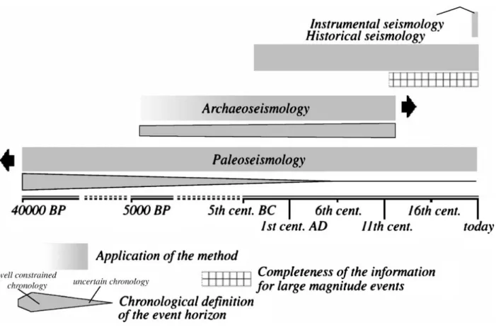
Three main branches of seismology investigate recent and past earthquakes: instrumental seismology,
historical seismology, and paleoseismology. To clarify the approximate temporal relationships of the
different branches, Figure 1.1 from Galadini et al. (2006) shows the temporal classification of the
different fields of expertise taking Italy as an example. As the time frames of the three disciplines overlap
and geological sciences as well as historical sciences are involved, interdisciplinary work is essential for
the study of past earthquakes.
2
Figure 1.1: Chronological intervals of application of different researches on past earthquakes in Italy. (Galadini et al. 2006).
Instrumental seismology started at the end of the 19th century (Rebeur-Paschwitz 1895, Wiechert 1926) and modern digital seismology is only about five decades old (Adams and Allen 1961, Bogert 1961). It is based on the exact measurement of ground motions with seismometers and today capable to deliver precise localization of the seismic source and reveal details of the source mechanism and rupture process, particularly through the application of numerical models and the inversion of complete ground motion records. However, in relation to the interseismic cycle, the time between two large earthquakes at the same fault, the time span covered by modern seismological data is extremely short.
Historical seismology is based on historical i.e. written information. Naturally the time frame of this
research is limited by the existence of a historical record, which can vary considerably from one cultural
region to another; e.g. in North America few centuries are covered, in the Levante the written record
extends several millennia (Ambraseys 1971). The interdisciplinary work with historians allows the
reconstruction of how past earthquakes were perceived by the population and/or damaged constructions
and infrastructure. Naturally the application is tied to populated area (Galadini et al. 2006).
3
Among the three disciplines paleoseismology covers the longest time span reaching back thousands or tens of thousands of years (McCalpin 1996). In paleoseismological research effects of earthquakes in the near surface lithology are investigated. If earthquakes of normal depth are strong enough, moment magnitude well above 6, they might leave persistent coseismic changes mainly in young sediments layers close to or at the activated fault line (McCalpin 1996). The stratigraphic record and precision of radiometric dating methods define the limit of the time frame for certain earthquakes (Ken-Tor et al.
2001). Paleoseismology is bound to locations close to active faults and is applicable only to earthquakes which are strong enough to change the structure of near surface deposits.
A new seismological discipline, often seen as a sub-discipline of paleoseismology (McCalpin 1996) is archaeoseismology, which focuses on archaeologically revealed information or traces which earthquakes left in persisting monuments. In the Encyclopedia of Solid Earth Geophysics archaeoseismology is defined as: “The study of pre-instrumental earthquakes that, by affecting locations of human occupation and their environments, have left their mark in ancient structures uncovered by means of archaeological excavations or pertaining to the monumental heritage.” by Hinzen (2011). Damaged buildings, rotated objects, collapse horizons and other archaeological evidence are the foundation for this kind of research.
The time frame covered is shorter compared to paleoseismology, but can be significantly longer than the written record. The research is limited by the existence of the remains of man-made structures, but these do not need to be directly at the causative fault of an earthquake, because ground motions capable of damaging buildings can reach many tens of kilometers and damage can occur during earthquakes smaller in size than necessary to be detected in paleoseismology (Galadini et al. 2006).
1.1 Archaeoseismology
De Rossi (1874), Lanciani (1918), Evans (1928) and Agamennone (1935) pioneered using archaeological information to investigate past earthquakes. Increasing numbers of publications dealt with the topic of seismogenic damage on man-made structures found in archaeological investigations (e.g. Karcz and Kafri 1978; Zhang et al. 1986; Guidoboni 1996). However, the early archaeoseismological publications were often of descriptive nature. Damage observed in man-made structures during archaeological excavation has been documented, attributed to earthquakes and interpreted by means of common sense. In the last decades, quantitative methods gained popularity addressing archaeoseismological questions with analytical approaches and the use of modern engineering seismological methods (Galadini et al. 2006, Hinzen 2009a).
For these tasks computer simulations have been used in a wide range of application and have proven to be
a useful tool in various ways. First models concentrated on investigating the dynamic response to ground
motion of basic structures such as free standing columns (Papastamatiou and Psycharis 1993, 1996,
4
Psycharis et al. 2000, Konstandinidis and Makris 2005, Hinzen 2009a). These structures are naturally vulnerable to ground-motion and in the first approximation have simple geometries which is an advantage, because it keeps the computation time in reasonable bounds.
A large part of archaeoseismological research is the analysis of damaged or deformed masonry, as this method of construction has been widely used in the past. The masonry can be of various styles of different time-periods. For example, walls made of polygonal blocks are considered to be more earthquake-resistant than walls built with rectangular blocks. Hinzen and Montabert (2017) tested this hypothesis by comparing the dynamic behavior of walls with varying height and width ratio (h/w-ratio) and four different block geometries when excited with analytical ground motion and measured earthquake records.
They confirmed that wall models with polygonal blocks have a higher earthquake resistance than the models with rectangular blocks. However, the authors made clear that the h/w-ratio is at least as important as the block geometry for the walls susceptibility to ground motion.
Not only the influence of the masonry style has been simulated in archaeoseismological research.
Numerical models are as well capable to investigate the dynamic behavior of more complex structures.
These simulations may also be linked with issues of cultural heritage preservation. Psycharis et al. (2003) analyzed the seismic behavior of the Parthenon Pronaos with discrete element models. In their study the multi drum columns of the temple were modeled with their existing imperfections to assess the vulnerability of the in situ state to ground motions. In addition, the effects of safety measures which are intended to increase the stability were simulated in terms of preservation of the architectural heritage. The simulations revealed that metal reinforcements support the drums of the columns against shear displacement, but are ineffective against uplift during stronger ground motions. In some cases, the reinforcements are counterproductive, suppressing the energy-dissipation of inter-drum movement. The authors could show that the imperfections have a severe influence to the stability of the columns and suggest eliminating those imperfections, to increase the stability.
Computer models are capable tools and it is therefore important to counter-check the validity of
simulation results. Cakti et al. (2016) compared the results of a shake-table test with the results of a
discrete element model. They constructed a 1/10 model of the Mustafa Pasha Mosque (Istanbul) on a
shake-table and modeled the same on the computer. Both models were excited with scaled seismograms of
the north-south component of the Montenegro earthquake (15.04.1979, M
W6.9). In total 26 tests were
carried out with both models. The authors showed that the analytical and experimental results were in
good agreement and concluded that the numerical simulation is also capable to calculate the realistic
response for full scaled building. Galvez et al. (2018) analyzed the behavior of a two-story masonry with a
discrete element model and a scaled model on a shake-table. The latter was excited with harmonic ground
5
motion in one horizontal direction with increasing frequencies. The response of the masonry was recorded by accelerometers. The same ground motion was used as boundary condition for the computer simulations. The simulated crack pattern and the point of collapse of both models are in good agreement.
The validation of computer simulations is an essential step in the development process. Instead of using shake-table tests, models can also be verified by comparing the simulated results with analytical solutions of known problems, the verification process is described in detail in Section 4.2 (Model Verification).
In archaeoseismology numerical models are not only applied to investigate the response of man-made structures to ground motions. The wide application range of these models also allows considering alternative damage scenarios. E.g. in Pınara (Turkey) a severely damaged Roman mausoleum is located in close proximity to a steep cliff. To test whether the damage was caused by an earthquake or a rockfall, Hinzen et al. (2013a) reconstructed the Mausoleum in a discrete element model based on a detailed 3D laser scan and historical information. Next to synthetic seismograms and analytical ground motions as boundary conditions to test the behavior of the model, additionally rockfall scenarios were simulated. The results of the simulations were compared with the in situ measured state of the Roman mausoleum. The authors revealed that a rockfall was not likely to produce the observed damage, but a local earthquake with a moment magnitude of 6.3 is a possible cause. An example where anthropogenic influence is likely the source for the observed damage was presented by Hinzen et al. (2010). The Lycian sarcophagus of King Arttumpara in Pınara is damaged and deformed; it is rotated by 6.37° off its original position.
Although parts of the damage pattern indicate an explosion, it was assumed that the coffin was rotated by an earthquake. A detailed discrete element model was developed based on a 3D laser scan of the Sarcophagus. Next to the response of the model to harmonic ground motions and recorded seismograms, also the effects of a blast on the Sarcophagus were simulated. The authors showed that a blast is likely the source of the observed rotation and could even reveal the amount of explosives used.
Computer models can also provide an opportunity to simulate secondary effects that are not related to damaged structures and still give valuable information about the ground motion history of a site. During archaeological excavation in Mycenaean Tiryns terracotta figures were found on the floor of a cult room and archaeologists hypothesized that the figures fell off a bench during an earthquake. Hinzen et al.
(2014a) developed a computer model to simulate the movement of these figures due to ground motions to
test the hypothesis that a damaging earthquake occurred in late Bronze Age. In the simulations many
scenarios were covered with a large parameter space. In total 74,250 individual tests were calculated to
cover all possible scenarios. The results revealed that in none of the simulated scenarios the outcome
matched the archaeological findings. Therefore, the earthquake hypothesis was refuted.
6
Figure 1.2 shows a general schematic workflow for a quantitative archaeoseismological investigation as it has been suggested by Hinzen et al. (2009). The model development relies mainly on two sections of input, first a reconstruction of the state of the investigated structure at the time when the potential earthquake occurred and second on boundary conditions such as earthquake ground motions and alternative causes. The latter are important, if it is not a priori clear that the observed structural damage is of coseismic nature.
For the reconstruction and quantification of damage of structural elements or complete buildings a precise documentation of the current state of the structure of interest is required (Schreiber and Hinzen 2010).
Today 3D laser scanner and digital photography are common tools for documentation (e.g. Schreiber et al.
2009, Hinzen et al. 2010, Schreiber and Hinzen 2010, Schreiber et al. 2012, Hinzen et al. 2013a, Hinzen
et al. 2013b, Hinzen et al. 2016a, Hinzen et al. 2018). Additional information from historical and
archaeological records complete the dataset for the reconstruction. The boundary conditions are derived
with geotechnical and seismological models based on geological, tectonic and geophysical information of
the site. Also site effects may be taken into account (Hinzen and Weiner 2009, Hinzen et al. 2016b,
Hinzen et al. 2018) for which explorative in situ measurements might be necessary (Hinojossa-Prieto and
Hinzen 2015). With the complete geotechnical model synthetic seismograms for specific earthquake
scenarios can be calculated and applied as input to models for the reconstructed structures.
7
Figure 1.2.: Schematic flow chart of quantitative archaeoseismic modeling (after Hinzen et al. 2009).
The center of the work scheme in Figure 1.2 is the model of the studied structure. Models based on the Finite Element Method (FEM) and DEM are established tools in engineering seismology to study the earthquake safety of contemporary buildings (Meskouris 1999, Meskouris et al. 2011); they can also be applied to study the behavior of (reconstructed) ancient structures. Their combination with the simulated earthquake scenarios and comparison with the (archaeologically) observed damage can help to find bounds for the parameters of the ground motion which once caused the damage (Stiros and Jones 1996, Galadini et al. 2006).
The reconstruction process heavily depends on the information that archaeologists and historians can
provide about the man-made structures. The dates of creation, destruction and/or abandonment of a site
define the time window for the damaging earthquake. Geologists and geophysicists provide information
about the tectonic environment, the seismicity and local earthquake site effects. These data are vital to
succeed with the quantitative approach to explore the potentially seismogenic damaging process. This
illustrates the importance of interdisciplinary work in archaeoseismological research.
8
1.2 Archaeoseismological Research in Israel
The wealth of archaeological sites in Israel fascinated researchers for more than 150 years. The Palestine Exploration Fund, founded in 1865 (https://www.pef.org.uk/history/, last accessed 03.08.2018) initiated surveys for the exploration of the Levante. In “The Survey of western Palestine.” Condor and Kitchner (1882) reported about their expedition from 1871–1878. They describe several archaeological sites in detail, of which numerous show damage, now associated to seismic activity (Karcz et al. 1977, Karcz and Kafri 1978, 1981). Karcz et al. (1977) first used the term archaeoseismic to relate to damage on archaeological structures attributed to earthquakes. A wide range of archaeoseismological research has been carried out in Israel.
The ancient city of Jericho is located north of the Dead Sea in vicinity to the Dead Sea Transform Fault (DSTF). Alfonsi et al. (2012) were able to identify two Neolithic (7,500-6,000 BCE) earthquakes at Tell es-Sultan by analyzing archaeological reports of the excavations. They could reconcile the archaeological findings with paleoseismological evidence of past earthquakes.
Figure 1.3: (a) Toppled columns of Hippos Sussita. (b) Dropped voussoir at the gate tower of Kalat Nimrod (Photos:
K.-G. Hinzen).
An often mentioned prime example for earthquake damage are the perfectly aligned toppled columns of the so called Cathedral at Hippos Sussita at the Sea of Galilee (Figure 1.3 (a)) (e.g. Stiros and Jones 1996, Hinzen et al. 2011, Wechsler et al. 2018). This is located on a ridge about 2 km east of the Sea of Galilee.
The perfect alignment of the columns was first misinterpreted as an indicator for the direction of ground
motion. With a scenario based numerical analysis Hinzen (2010) showed that this hypothesis does not
apply. The main earthquake that affected the site happened in 749 C.E. (Marco et al. 2003).
9
Wechsler et al. (2009) associated the same earthquake with the destruction of the synagogue of Umm-El- Qanatir. It is located about 10 km north-east of Hippos Sussita. The authors’ main arguments are the abandonment of the close city Umm-El-Qanatir and a probable landslide, triggered by the earthquake. The synagogue was excavated by Kohl and Watzinger (1916) and is currently in the process of an elaborate anastylosis.
The 749 C.E. earthquake also impacted the western shore of the Sea of Galilee. In ancient Tiberias Marco et al. (2003) identified seismogenic damage at the Galei Kinneret excavation. The archaeological stratigraphy dates the damage in a time around the 749 C.E. earthquake. The authors showed that the findings are in good agreement with paleoseismic and historic evidence.
In northern Israel lies the Nimrod Fortress (or Kalat Nimrod). It was constructed in 1228 to control the valley between Mount Hermon and the rest of the Golan Heights, a former route from the Galilee to Damascus (Ellenblum 1989). The fortress was heavily damaged during the 1759 Lebanon earthquake.
Many arches inside the ruin show damage, which are a strong indicator for a seismogenic origin.
Keystones or voussoirs slipped from their original position (Figure 1.4 (b)). This is in particular evident in the so called “secret passage” of the gate tower, where the voussoirs slipped over a 20 m long section.
Kamai and Hatzor (2008) tested the dynamic characteristics of the type of arches found in Nimrod with a discontinuous deformation analysis. They estimated a PGA of 0.4 g at 1 Hz to allow movement of the keystones or voussoirs. During a visit to the fortress one might get the impression that the grade of damage depends on the orientation of the according arches. Hinzen et al. (2016a) systematically examined the damage of 95 arches but could not confirm a dependency between the grade of damage and orientation of the arch.
1.3 Two Case Sites in Israel
In the course of this work two archaeological sites in Israel are studied in detail; both are located north of the Sea of Galilee and considered to show earthquake damage. The chosen sites are considered to be damaged by earthquakes (Fischer et al. 1984, Ellenblum et al. 1998). To document the current state of the sites they have been carefully surveyed with a 3D laser scanner, to get a detailed virtual 3D model of the damaged structures.
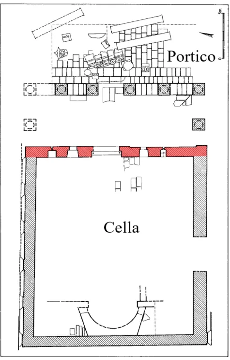
The first structure is the ruin of the Roman Temple of Kedesh, whose remains are currently in precarious
stable condition (Figure 5.2 (c) and (d)). The temple was destroyed during an earthquake on May 19th 363
C.E. (Fischer et al. 1984). At this particular site information about the initial state of the Temple at the
time of the earthquake is unclear and in addition the remains were heavily altered by anthropogenic
influence (i.e. looting). A reconstruction of the process which caused the destruction is hardly possible.
10
For such sites with an unknown history of destruction the regular archaeoseismological approach described above with an elaborate reconstruction process is not feasible. Figure 1.3 shows numerous examples of damaged archaeological sites in currently stable conditions.
However, despite these problems it is still possible to derive information about the ground motion history from such sites. Not only archaeological remains can be in delicate stable states; under specific circumstances natural formations can also be in precarious condition. Precariously balanced rocks (PBR) are used as seismoscope to expand the knowledge of the ground motion history of a specific site (e.g.
Figure 1.4: Examples of precariously balanced archaeological structures: (a) ruin of the Roman harbor bath in
Ephesus, Turkey; (b) pre-Roman rock cistern at Patara, Turkey; (c) ruin of Montfort Crusader castle, Israel; (d)
Lycien sarcophagus Xanthos, Turkey; (e+f ) Mycenaean corbeled vault, Tiryns, Greece; (g) ruin of Cyclopean wall
of Tiryns, Greece; (h) Roman mausoleum Pınara, Turkey; (i+k) ruins of Roman bath Pınara, Turkey; (l) delicate
Roman arch, Patara, Turkey (after Schweppe et al. 2017; Photos: K.-G. Hinzen)
11
Brune 1996, Anooshehpoor 2004). In this work the concept of PBR is adapted for archaeological structures that are in a fragile condition.
Thus the ruin of the Roman Temple at Kedesh was considered a Precariously Balanced Archaeological Structure (PBAS) (Schweppe et al. 2017). The focus in this approach is not on the ground motion that destroyed the Roman Temple, but on the nature of the ground motions that did not topple the remains during the past 17 centuries. This method allows utilizing former not necessarily usable archaeological structures to gain information about the ground motion history of a site.
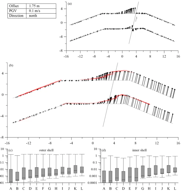
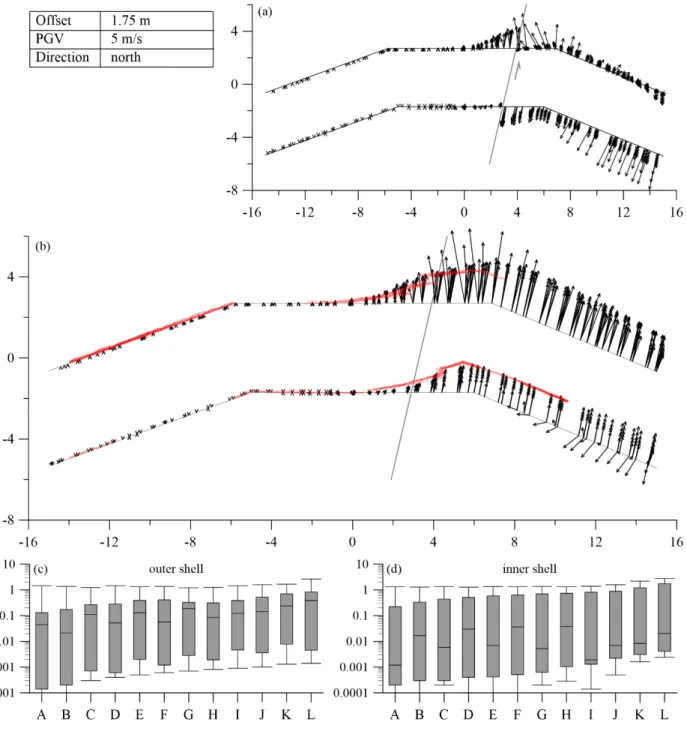
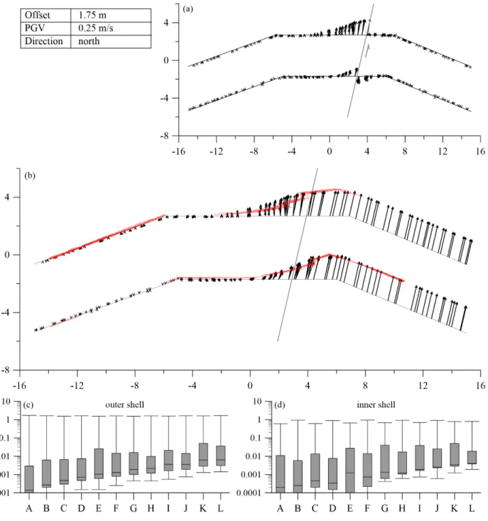
The second site is the ruin of the Crusader Fortress at Tell Ateret, a prominent archaeoseismological research site. Frankish Crusaders started the construction of a fortress directly on top of the DSTF fault line (Ellenblum et al. 1998). The fortress was still under construction when it was conquered by Muslim forces in 1179 and subsequently abandoned. Today the massive fortification walls are offset by tectonically caused movements along the fault. The fortification wall is 4.4 m wide and of double shell nature. The volume between the shells is filled with a mixture of basalt cobles and mortar. While previous work concentrated on the sequence of earthquakes at Tell Ateret since Iron Age II (Marco et al. 1997, Ellenblum et al. 1998, 2015), details of the rupture process which deformed the northern fortification wall of the fortress is the core of this study. Therefore, a complex model has been developed, which is capable to simulate the movement of the walls, where the filling in between demanded special attention. With the final model, which is comprised by 52,864 individual blocks, various different scenarios were considered in the simulations. So far, exclusively two earthquakes have been assigned to the observed deformation of the fortification walls, based on the good agreement between the age of the archaeological structures at the site and the date of the known past earthquakes. The possibility of creeping motion has been disregarded, although creeping is known to exist along sections of the DSTF (Hamiel et al. 2016). Questions about the dislocation velocity at the fault and the amount of movement of each plate were addressed by the DEM model of the wall. Information about the dislocation velocity and the displacement of the fault are important parameters for inferring the magnitude of the past earthquakes.
In total three different software solutions were used for the model development of both sites. However,
not all approaches proofed functional. The development process for each model is described in the
according chapters.
12
1.4 Guidelines of the Thesis
Following to this introduction Chapter 2 gives a geographical and geological overview of the study areas in Israel. It also includes an introduction to the tectonic setting and instrumental and pre-instrumental seismicity. The next two Chapters cover the methods used in this work. Chapter 3 describes the basic concept of Laser Scanning Technique and its applications. Chapter 4 gives a detailed overview of Computer Models based on the DEM and the development process for all software solutions used in the course of this work. Chapter 5 is split into two mayor sections, each dealing with one site. In the first section background information about the Roman Temple of Kedesh are given. Afterwards the surveying and the modeling process are described in depth and the results of the simulations are presented and discussed. The second section deals with the ruin of the Crusader Fortress of Tell Ateret. Here the same logical sequence as in the preceding section is followed. Lastly the discussion and conclusion, in which the results of both sites and the application of the DEM are considered in a wider angle of archaeoseismology is presented, closing with recommendations for further research.
The Thesis was partly funded by the German Israeli Foundation (GIF) Grant Number 1165. As part of the
Itasca Education Program (IEP) Itasca provided the software licenses for 3DEC.
13
2 R EGION OF I NTEREST
This chapter gives an introduction to the area, where the selected archaeological sites are located. A short geographical and geological overview is followed by a description of the current tectonic setting and the pre-instrumental and instrumental seismicity.
2.1 Geographical Overview
Israel is located in the Middle East on the south-eastern shore of the Mediterranean Sea and the northern shore of the Red Sea. It has a surface area of 22,072 km
2including the disputed territories (www.cbs.gov.il last accessed 07.2017). The country has an elongated approximate triangular shape. From north to south the country is about 430 km long. The widest east-west extension is 115 km and the narrowest is 15 km.
The largest perennial river in Israel is the Jordan River. It is feed by three source flows: Hasbani, Dan and
Banyas in the north and discharges into in the Dead Sea (Heimann and Sass 1989). On its way south the
Jordan River crosses the Hula Basin (also Hula Valley), a former wetland which was drained for
agricultural use in the 1950s. Prior the drainage the Hula Basin was the site of Lake Hula, the
northernmost of originally three natural inland water bodies connected by the Jordan River (Hambright
and Zohary 1998). The Hula Basin subsides along the DSTF and lies at an elevation of about 70 m. The
flanks of the Golan Heights and the Upper Galilee (Naftali) mountains form the boundaries of the Hula
Basin to the east and west respectively (Horowitz 1973). South, the basin is closed by a basalt block,
which throttled the water flow downstream through the Jordan Gorge to the Sea of Galilee, which caused
the historic wetlands (Hambright and Zohary 1998). The Jordan Gorge is a straight narrow gorge
connecting the Hula Basin over approximately 10 km with the Sea of Galilee (Figure 2.1 (b)). Between
the Sea of Galilee and the Dead Sea lies the Jordan Valley. The Dead Sea is a hyper-saline lake, the shore
line is about 430 m (as of 2016 https://isramar.ocean.org.il/ last accessed 10.2018) below sea-level
(Quennell 1956a), which makes it the lowest point on land on Earth. South of the Dead Sea is the Araba
Valley, another depression, that extends to the south to the Gulf of Aquaba, which opens into the Red Sea.
14
Figure 2.1: Digital terrain map of the DSTF (black lines), the single headed black
arrows indicate the movement along the DSTF. The white rhombus marks the epicenter
of the synthetic JVF earthquake (cf. Chapter 5); (RS = Red Sea, GoS = Gulf of Suez,
GoA = Gulf of Aquaba, DS = Dead Sea, SG = Sea of Galilee, JVF = Jordan Valley
Fault). The arrows indicate the rift movement of the GoS and RS rift, respectively. The
dashed grey line marks the oceanic ridge. The black rectangle indicates the working
area shown in (Figure 2.5) (after Schweppe et al. 2017).
15
Figure 2.2: Multi-annual average of the temperature and precipitation in Israel. The blue line shows the monthly average precipitation (mm/m
2) for the period 1981-2010. The red bars show the monthly average temperature (°C) of the years 1995 -2009 numbers on top and bottom are the minimum and maximum average temperatures measured in Israel (data from:
www.cbs.gov.il last accessed 07.2017).
The Mediterranean climate of the region is characterized by hot dry summers and mild wet winters.
Figure 2.2 shows average precipitation and temperatures of Israel by month. The annual average precipitation is 437 mm/m
2, for comparison the total average in Germany for the years 1961 to 1990 is 848 mm/m
2(https://de.statista.com, last accessed 05.2018). The seasonal temperature has a variance between minimum and maximum of about 15°C (www.cbs.gov.il last accessed 07.2017).
2.2 Geological Overview
The geologic map shown in Figure 2.3 gives an overview of the geology of Israel. The oldest rock
formations are exposed in southern Israel and in northern direction the formation are getting younger. The
oldest rocks are magmatic and metamorphic rocks of the Precambrian. Younger magmatic rocks are from
Neogene and Pleistocene and are mostly exposed in the north, except of some locations in the east. The
majority of the rocks are limestone from Mesozoic and Cenozoic times. In Figure 2.3 it is evident,
especially in the Precambrian formations, that pre-Miocene formations are offset. The formations in
eastern Israel are shifted further north than west, which is the consequence of the left-lateral movement
along the DSTF (Quennell 1959, Freund 1965, Freund et al. 1970, Bartov et al. 1980).
16
Figure 2.3:Geologic Map of Israel (1:500.000)
(from http://www.gsi.gov.il, last accessed 08.2018,
corrected stratigraphy).
17
Following Garfunkel (1988) the geologic evolution of Israel can be structured into three main parts.
1. Late Precambrian Pan African orogenic stage 2. Early Cambrian to End-Paleogene platformal stage 3. Early Neogene to Recent rifting stage
The orogenic stage contains the oldest rock formations, the rocks are exposed in southern Israel in the area of Elat and in the surrounding of the Red Sea (cf. Figure 2.3), they belong to the Arabo-Nubian Shield (Picard 1939). The rocks can be separated into two complexes, the orogenic and the late-orogenic complex. The first consists of metamorphic and plutonic rocks. The metamorphic rocks were heavily influenced by the events of the Pan-African orogeny (Matthews et al. 1989), the metamorphism reached high greenschist to middle amphibolite grade (Garfunkel 1988). With the ending of the main activity of the orogeny a widespread plutonic phase started, marking the main consolidation phase of the crust (Garfunkel 1988). The plutonic phase was followed by uplift and erosion. The late-orogenic complex is mainly composed of unmetamorphed sediments, high-level intrusions and volcanic rocks (Garfunkel 1988).
The platformal stage extends over a long time period from the end of the Pan-African Orogeny in early Cambrian to the onset of the rifting in Miocene, which includes the Paleozoic and Mesozoic eras in their entirety and the early Cenozoic era. The transition from the orogenic to the platformal stage began with an uplift followed by massive erosion, which formed a large peneplain. Only some resistant volcanic rock formations in southern Israel did not erode and formed hills of several hundred-meter height. After the initial erosion period the area was coined by vertical movement and global sea level changes (Garfunkel 1988). Periods of sedimentation were separated by phases of erosion; also phases with tectonic and magmatic activity occurred. In Israel Paleozoic sediments, mostly sandstones from continental and shallow marine environments are exposed in southern Israel, in the southern Negev, other deposits eroded (Garfunkel 1988). In Mesozoic time, between Later Permian and early Jurassic (Liassic) the tectonic setting changed with the breakup of Pangaea, which led to two major changes in Israel: from the Late Permian, the subsidence towards the Mediterranean continental margin increased and between Triassic and Liassic times there was differential movement, rifting and magmatism, which are associated with the formation of the Mediterranean passive continental margin (Garfunkel and Derin 1984, Garfunkel 1988).
The tectonic-magmatic activity ended in Middle Jurassic, followed by subsidence, which usually
increased towards the continental margin and led to sedimentation under both shallow and deep water
conditions. In Latest Jurassic the sedimentation phase ended by the activity of an intra-plate hot-spot
18
causing widespread magmatism, regional uplift and erosion. This phase lasted until Early Cretaceous and eroded the older shallow-water deposits (Garfunkel 1988). In Cretaceous times the sea level rose and a phase of extensive sedimentation of mostly limestone and dolostone began (Sass and Bein 1982, Garfunkel 1988). In the Late Cretaceous and Paleogene, the sedimentation shifted and chalk and marl became the dominant sediments.
The rifting stage was initialized by a significant change in the tectonic setting in the Neogene.
The breakup of the Arabo- African continent with the onset of the rifting at the Red Sea and Gulf of Suez created new plate boundaries in the region, the movement along the DSTF started. A schematic representation of the initial tectonic setting and the movement directions of the plates has been given by Garfunkel (1988) (cf. Figure 2.4). The tectonic activity uplifted large areas above sea level and was accompanied by widespread magmatic activity, particularly east of the DSTF. In Middle Miocene during an active volcanic phase the so called ‘Lower Basalt’ originated (Steinitz et al. 1978, Garfunkel 1988). In Pliocene another volcanic outburst covered a large area in southern Galilee and in the Golan heights with a basalt flow, this sequence is also called
“Cover Basalt” (Steinitz et al. 1978, Garfunkel 1988). Between the volcanic events short phases of sedimentation are known. Today the pre-miocene formations from the pre-rifting stage are offset 105 km by the DSTF (Quennell 1959, Freund 1965, Freund et al. 1970, Bartov et al. 1980).
Figure 2.4: Schematic block model of the initial tectonic setting at the
beginning of the Mid-Cenozoic to Recent rifting stage. The movement along
the DSTF allows the rifting systems to open (after Garfunkel 1988).
19
2.3 Tectonic
The tectonic system of Israel has been subject of geological research over 100 years (Suess 1891, Gregory 1921, Willis 1928). In the first publications the DSTF was also called “Dead Sea Rift”, because the depressions (such as the Dead Sea, Sea of Galilee, Hula Basin), located along the fault line, have been misinterpreted as a consequence of ramps or rifting (Willis 1928). However, the depressions are pull-apart basins and result from the movement along the DSTF (Ben-Avram and Schubert 2006).
The DSTF is a left lateral transform plate boundary, which separates the Sinai subplate in its west from the Arabian plate in the east (Figure 2.1 and Figure 2.4). The fault line of the DSTF strikes north-south and connects the Red Sea in the south over a distance of 1000 km with the Anatolian Faulting System of the Bitlis-Zagros collision zone in the north (Quennell 1956b, Freund et al. 1968). GPS observations reveal that both plates are moving in northern direction separating from the Nubian Plate with different speeds (e.g.
McClusky et al. 2003, Wdowinski et al., 2004;
Mahmoud et al. 2005, Reilinger et al. 2006, Vigny et al. 2006, Le Beon et al. 2008), the movement of the plates is connected with the extensional regime of the Red Sea and the Gulf of Suez. The opening speed of the Red Sea rift varies from 14 ± 1.0 mm/yr at 15°N to 5.6 ±1.0 mm/yr at 27°N (McClusky et al.
2003). And the opening speed of the Gulf of Suez is 1.5 ± 0.4 mm/yr (Mahmoud et al. 2005). The consequence of the different rifting speeds is the left-lateral strike slip movement observed at the DSTF (Figure 2.4). GPS measurements revealed an overall short term sinistral slip rate of 4-6 mm/yr (Wdowinski et al. 2004, Gomez et al. 2007a, Sadeh et al. 2012), which matches the long term geologic rates estimated by the 105 km offset of the geologic features (Quennell 1956b, Freund 1965, Bartov et al.
1980).
Figure 2.5: Working area; the red stars mark the location of
the Roman Temple of Kedesh and the Ruin of the Cursader
Fortress Ateret. Black lines show the local active strands of
the DSTF (after Wechsler et al. 2014) (JGF = Jordan Gorge
Fault, HCF = Hula Basin Central Fault, HBF = Hula Basin
Border Fault, RaF = Rachaya Fault, RF = Roum Fault, YF =
Yammouneh Fault, CF = Carmel Fault). The white
rhombuses mark the epicenters of the sources used to
calculate synthetic seismograms.
20
In Israel the DSTF is segmented into three main parts, named after the depressions; from south to north:
the Araba Valley, the Jordan Valley and the Hula Basin (Figure 2.1). Between Araba Valley and Jordan Valley lies the Dead Sea; the Jordan Valley and the Hula Basin are separated by the Sea of Galilee and the Jorden Gorge, which connects the Sea of Galilee and the Hula Basin. In the Hula Basin the DSTF splays into several non-parallel faults. The most prominent branches from east to west are the Rachaya Fault (RaF), Yammouneh Fault (YF) and the Roum Fault (RF) (Figure 2.5). In the so called Lebanese Restraining Bend (LRB) the deformation is partitioned between the strike-slip movement and crustal deformation (Gomez et al. 2007b). The slip rate along the sections of the DSTF is not constant (McClusky et al. 2003, Sadeh et al. 2012). Sadeh et al. (2012) analyzed the GPS data of 33 permanent and 145 survey GPS stations measured over 12 years. They were able to show that the slip rate and the locking depth of the DSTF tends to decrease from south to north. In the Araba Valley section they estimated a slip rate of 5.1 mm/yr and locking depth of 15.5 km. In the Dead Sea the slip rate decreased to 4.8 mm/yr and the locking depth was at 14.1 km. In the Jordan Valley segment itself the slip rate and locking depth was not uniform, the southern section had a slip rate of 4.9 mm/yr and a locking depth of 15.8 km was measured and in the northern part only a slip rate of 3.8 mm/yr and a locking depth of 12.4 km. In the Jordan Gorge Fault (JGF) they estimated a slip rate of 3.7 mm/yr at a locking depth of 8.7 km. In their study the authors also identified oblique motion at the Carmel Fault System (CFS) a fault system located west of the DSTF.
A left-lateral motion of 0.7 mm/yr and extension rates of 0.6 mm/yr were measured. The authors concluded that lateral movement of the DSTF is inferred to the CFS, resulting the significant decrease of the slip-rate within the Jordan Valley. In their study Sadeh et al. (2012) found a good agreement between the geodetically estimated locking depth and the depth, above which 90% of the seismic moment has been released, which underpins the estimated locking depth. Hamiel et al. (2016) identified in their geodetic analysis of GPS data a shallow creep motion in the northern section of the Jordan Valley Fault (JVF), where Sadeh et al. (2012) measured the slower slip rate. They estimated creep movement in a depth up to 1.5 ± 1 km with a creep rate of 2.5 ± 0.8 mm/yr.
2.4 Seismicity
The seismicity of Israel is characterized by infrequent large earthquakes with periods of small to moderate earthquakes in between (Begin et al. 2005, Agnon 2014). This section first presents measures for the strength of earthquakes that are important for this work, followed by the description of the pre- instrumental and instrumental seismicity of Israel.
2.4.1 I NTENSITY
The macroseismic intensity is a classification of the severity of earthquake ground motion in a certain area
(e.g. Wood and Neumann 1931, Sieberg 1933, Medvedev et al. 1964, Grünthal 1998). It is based on
21
people’s perception of the event and the effect that the ground motions have on man-made structures.
Although the macroseismic maps based on these scales are biased by the proximity or lack of populated areas to the epicenter, construction types of the affected structures and local site effects, they are often the only measure able to estimate the strength of pre-instrumental earthquakes. Most intensity scales have twelve degrees, labeled with Roman numbers. The most prominent scales are the Modified-Mercalli scale (MM) introduced by Wood and Neumann (1931), the Medvedev-Sponheuer-Karnik scale (MSK) by Medvedev et al. (1964) and the European Macroseismic Scale (EMS-98) by Grünthal (1998). Table 2.1 lists the short form of the twelve intensities of the European Macroseismic Scale (Grünthal 1998).
Table 2.1: Short form of the European Macroseismic Scale EMS-98 (Grünthal, 1998).
# Definition Description of typical observed effects I Not felt Not felt
II Scarcely felt Felt only by very few individual people at rest in houses
III Weak Felt indoors by a few people. People at rest feel a swaying or light trembling.
IV Largely observed
Felt indoors by many people, outdoors by very few. A few people are awakened. Windows, doors and dishes rattle.
V Strong Felt indoors by most, outdoors by few. Many sleeping people awake. A few are frightened. Buildings tremble throughout. Hanging objects swing considerably.
Small objects are shifted. Doors and windows swing open or shut.
VI Slightly damaging
Many people are frightened and run outdoors. Some objects fall. Many houses suffer slight non-structural damage like hair-line cracks and fall of small pieces of plaster.
VII Damaging Most people are frightened and run outdoors. Furniture is shifted and objects fall from shelves in large numbers. Many well built ordinary buildings suffer moderate damage: small cracks in walls, fall of plaster, parts of chimneys fall down; older buildings may show large cracks in walls and failure of fill-in walls.
VIII Heavily damaging
Many people find it difficult to stand. Many houses have large cracks in walls.
A few well-built ordinary buildings show serious failure of walls, while weak older structures may collapse.
IX Destructive General panic. Many weak constructions collapse. Even well-built ordinary buildings show very heavy damage: serious failure of walls and partial structural failure.
X Very destructive
Many ordinary well-built buildings collapse.
XI Devastating Most ordinary well-built buildings collapse, even some with good earthquake resistant design are destroyed.
XII Completely devastating
Almost all buildings are destroyed.
22
Another approach is the Environmental Seismic Intensity scale (ESI 2007) developed under the patronage of International Union for Quaternary Research (INQUA) (Michetti et al. 2007). Contrary to the above intensity scales, this is not based on the impact of an earthquake to human environment, but on the size and distribution of earthquake environmental effects, such as surface rupture, liquefaction or tree shaking.
The ESI 2007 is intended to be a supplement to the other Intensity scales.
2.4.2 M AGNITUDE
In modern seismology the strength of instrumentally recorded earthquakes is quantified by magnitude. In 1935 Charles Richter published a magnitude which was based on instrumental measurements. His intention was to develop a measure “freed from uncertainties of personal estimates or the accidental circumstances of reported effects” (Richter 1935). He introduced the local magnitude (M
L) which is based on the maximum amplitude of a seismogram measured with a Wood-Anderson-Seismometer and the epicentral distances.
The surface-wave magnitude (M
S) was introduced by Gutenberg and Richter (1956). It is based on the measurement of the amplitudes of surface waves at certain periods. Empirical relations allow to estimate M
Sfrom intensities derived from the historical record (e.g. Ambraseys and Melville 1988), which makes it valuable for the magnitude estimation of pre-instrumental earthquakes. However, it is important to point out that the empirical relationships are not globally valid, but refer to the specific regions for which they were developed.
Another important magnitude is the Moment Magnitude (M
W) introduced by Hanks and Kanamori (1979).
This measure is not based on the decline of the amplitude over distance, but on the seismic moment (M
0) and is defined as:
𝑀𝑀
𝑤𝑤= (log 𝑀𝑀
0/1.5) − 6.07 (Eq. 2.1)
where 𝑀𝑀
0is defined as (Aki, 1966):
𝑀𝑀
0= 𝜇𝜇𝜇𝜇𝜇𝜇 (Eq. 2.2)
where µ is the shear-modulus (Pa) of the involved rocks, 𝜇𝜇 is the rupture area (m²) and 𝜇𝜇 is the average
displacement (m) on the rupture area.
23
2.4.3 P RE -I NSTRUMENTAL E ARTHQUAKES
The region around the DSTF is rich on information of pre-instrumental earthquakes (Agnon 2014). These are spread over three main archives; the historical, geological and archaeological archive. The historical record in Israel reaches back about 2000 years and provides comprehensive information about the seismic history of the area (Ambraseys 1971). Numerous research studies and historical earthquake catalogs are based on this record (e.g. Ambraseys et al. 1994, Guidoboni et al. 1994, Karcz 2004, Ambraseys 2005, Guidoboni and Comastri 2005, Sbeinati et al. 2005). The geological archive forms the basis of paleoseismological investigations. Both on-fault effects (e.g. Reches and Hoexter 1981, Marco et al. 2003, Meghraoui et al. 2003, Daëron et al. 2005, Wechsler 2014) and off-fault effects (e.g. Marco et al. 1996, Shaked et al. 2004, Agnon et al. 2006) are the subject of the research. The archaeological archive includes archaeological sites that have potential seismogenic damage. Karcz et al. (1977) compiled a list of sites that show evidence of seismic activity along the DSTF. In numerous further studies potential seismogenic damage on archaeological sites was investigated (e.g. Marco et al. 1997, Ellenblum et al. 1998, Marco et al. 2003, Shaked et al. 2004, Thomas et al. 2007, Wechsler et al. 2009, Sbeinati et al. 2010, Ferry et al.
2011, Hinzen et al. 2016a).
With this wealth of information from interdisciplinary and independent research it was possible to compile earthquake catalogs for the last 2000 years (e.g. Garfunkel 1981, Ambraseys and Barazangi 1989, Ben- Menahem 1991, Klinger et al. 2000a, Migowski et al. 2004, Wdowinski et al. 2004, Marco et al. 2005, Marco and Klinger 2014, Ellenblum et al. 2015). Table 2.2 summarizes studies of 31 on-fault earthquakes for the DSTF over the last 2000 years validated by interdisciplinary studies.
Table 2.2: List of on-fault palaeoseismic investigations at the DSTF system arranged by year of publications (after Marco and Klinger 2014). Bold letters indicate earthquakes used to simulate ground motions in this study.* unless
indicated different all dates are Common Era (CE).
#
Reference SegmentAchievement Earthquake*/Slip Rate (SR)/
Last Event (LE)/ Recurrence (Re)
1 Reches and Hoexter (1981) S. Jordan Valley 31 BCE, 747
2 Marco and Agnon (1995) Dead Sea Re
3 Amit et al. (1996, 1999, 2002) S. Araba Valley Re
4 Marco et al. (1997, 2005); Ellenblum et al.
(1998) Jordan Gorge 1202, 1759
5 Galli (1999) Araba-Jordan-Hula Valley
6 Enzel et al. (2000) Dead Sea Re
7 Klinger et al. (2000a) N. Araba Valley 1212
24
#
Reference SegmentAchievement Earthquake*/Slip Rate (SR)/
Last Event (LE)/ Recurrence (Re)
8 Klinger et al. (2000b) N. Araba Valley SR
9 Niemi et al. (2001) N. Araba Valley SR
10 Zilberman et al. (2000) Hula Valley
11 Gomez et al. (2001, 2003) Serghaya Fault 1705 or 1759
12 Meghraoui et al. (2003) Misyaf, Yammouneh
13 Marco et al. (2003) Sea of Galilee 749
14 Daëron et al. (2004, 2005, 2007) South Yammouneh 1202
15 Zilberman et al. (2005) S. Abara Valley 3/1068/
16 Marco et al. (2005) Jordan Gorge 1202, 1759/LE/SR
17
Chorowicz et al. (2005) Yammouneh SE18
Akyuz et al. (2006) Northern Yammouneh 859, 1408, 187219 Nemer and Meghraoui (2006) Roum Fault 1837, SR
20 Haynes et al. (2006) N. Araba Valley 634 or 659/660, 873, 1068 and
1546
21 Elias et al. (2007) Lebanon thurst 551
22 Thomas et al. (2007) Aqaba
23 Ferry et al. (2007) Jordan Valley SR
24 Le Beon et al. (2008) Araba Valley
25 Nemer et al. (2008) Rachaya and Serghaya
faults 1759
26 Makovsky et al. (2008) Elat Fault SR
27 Altunel et al. (2009) S. Turkey SR
28 Le Beon et al. (2010) Araba Valley SR
29 Karabacak et al. (2010) Northern Yammouneh SR
30 Ferry et al. (2011) Jordan Valley SR, Re, LE
31 Le Beon et al. (2012) Araba Valley SR