Discrete Inverse Sobolev Inequalities with Applications to the Edge and Face Lemma for the Finite Element Method

(1)

Research Collection

Master Thesis

Discrete Inverse Sobolev Inequalities with Applications to the Edge and Face Lemma for the Finite Element Method

Author(s):

Bringmans, Levie Publication Date:

2020-02-09 Permanent Link:

https://doi.org/10.3929/ethz-b-000401981

Rights / License:

In Copyright - Non-Commercial Use Permitted

This page was generated automatically upon download from the ETH Zurich Research Collection. For more information please consult the Terms of use.

ETH Library

(2)

Discrete Inverse Sobolev Inequalities with Applications to the Edge and Face Lemma for the Finite Element

Method

Master’s Thesis Levie Bringmans February 9, 2020

Advisor: Prof. Dr. Ralf Hiptmair Department of Mathematics, ETH Z¨urich

(3)

(4)

Abstract

In this thesis we set out to prove certain inverse inequalities for piece- wise linear Lagrangian finite element spaces. More specifically, we give a proof of the edge lemma and face lemma from [23]. First we discuss some preliminaries on Sobolev spaces and the finite element method. Then we move on to the main part of the thesis concerning newly discovered results and proofs which is the content of Chapters 4 and 5. In Chapter 4 well-known inverse inequalities are stated and proved together with some essential new ones for certain slices through centroids of tetrahedral elements. In chapter 5 we discuss some erroneous proofs of the edge and face lemma from certain research papers followed by our own proofs of these lemmas together with some key inverse inequalities. We conclude everything by giving a detailed exposition of results which use the edge and/or face lemma.

(5)

Acknowledgements

First and foremost I would like to thank my thesis advisor professor Dr.

Ralf Hiptmair for proposing a project that was not only challenging but also very close to current research. I’m not going to lie, setting out with the sole task to prove certain results as my master’s thesis was a bit daunting at first. A thought which popped up in my mind countless times was a variant of ’What if I’m not able to prove these results or what if I’m only able to give a partial solution?’. It took me a couple of weeks to gather my thoughts and figure out a way to attack the problems that I was given head on. Thankfully professor Hiptmair made time for coaching me which was very helpful because I had little prior experience on the topic of inverse inequalities. After putting in a lot of effort to catch up on the necessary concepts and definitions I was able to derive new results on a high technical level which required a lot of scientific creativity. I combined these results to derive a proof of the edge and face lemma which albeit quite long, is in essence surprisingly elegant.

Next I would like to thank my parents for giving me the opportunity to study abroad at ETH Z¨urich. Studying abroad at ETH has been a wonderful experience which I will cherish for the rest of my life. I would finally like to thank Dr. Jonas Bekaert for introducing and helping me work with the vector graphics editor Inkscape which was an essential part of the construction of the figures in this thesis. I would also like to thank him for the many chats we had during this period which helped me unwind a bit and keep my mind off my work.

ii

(6)

Chapter 1 Introduction

In this thesis we are interested in a theoretical aspect of the finite element method. The finite element method uses finite dimensional function spaces to construct approximations to solutions of partial differential equations. The fact that these spaces are finite dimensional allows us to use norm equivalence to obtain so-called inverse inequalities. The tricky part is therefore not proving that such inequalities exist but rather getting an explicit expression for these inequalities in terms of the mesh parameters.

The norms in which we are interested are Sobolev andL^p-norms because they are associated to the natural function spaces used for analyzing the finite element method. We will be mainly interested in two specific inverse inequalities, namely the edge and face lemma. The inequalities in these lemmas state a logarithmic bound in terms of the mesh parameters on a certain Sobolev norm of a restriction of a finite element function. The interesting fact to notice here is the logarithmic bound. Such a factor usually only appears in inverse inequalities for two-dimensional domains while the edge and face lemma hold for three-dimensional domains.

Our main objective is to give a complete proof of the edge and face lemma.

Currently, there is no known complete proof of these results. However, they are used in current research to prove estimates on the condition number of certain preconditioners resulting from finite element discretization.

The proofs that we will give will be quite detailed to highlight the fact that there aren’t any ambiguities anywhere. The problem with the current proofs of the edge and face lemma is a spurious use of certain inverse inequalities. It would be counterproductive to claim that we have found a correct proof while omitting many of the details. This is precisely what lead to the errors in the known proofs.

In the final chapter we will be less concerned with detailed proofs because all results stated are from research papers and therefore not our own. They also

(11)

1. Introduction

do not contribute to the proofs of the edge and face lemma. This chapter is mostly an exposition of the results which use the these lemmas. It also highlights the importance of these results and that giving a proof actually bridges a gap between theory and experiment.

2

(12)

Chapter 2 Preliminaries

2.1 The Euclidean Norm and Volume in R

ⁿ

In this section we introduce notation that we will use very frequently. We start by fixing the notation for Euclidean norms.

Definition 2.1 (Euclidean norm) The Euclidean norm of a vector x= (x1, . . . , xn)^T ∈Rⁿ is defined as

|x|:=

n

X

k=1

x²_k

!1/2

.

Next we fix the notation for the surface area and volume of a set.

Definition 2.2 (Volume) Let Ω⊆Rⁿ be a Borel-measurable set. We define the volume of Ω as

vol_n(Ω) :=

ˆ

Rⁿ

1_Ω(x)dx= ˆ

Ω

dx, where dxis the Lebesgue measure on Rⁿ.

Remark. For n= 2 we will refer to vol2(Ω) as the surface area of Ω.

2.2 L

^p

-spaces

In this section we define the elementaryL^p-spaces which we will do in full gen- erality. However, we will only need the special case of the Lebesgue measure for all our results.

Definition 2.3 Let (Ω,F, µ) be a measure space andp >0 and integer. The corresponding L^p-spaceis defined as

L^p(Ω,F, µ) =

u: Ω→R|uisF-measurable, ˆ

Ω

|u|^pdµ <+∞

,

(13)

2. Preliminaries

where as usual we understand f as the equivalence class of functions which areµ-a.e. equal to f.

The norm

kuk_Lp(Ω,F,µ):=

ˆ

Ω

|u|^pdµ 1/p

, ∀u∈L^p(Ω,F, µ), turns L^p(Ω,F, µ) into a Banach space.

Notation: For (Ω,F, µ) = (Ω,B(Ω), λ) where Ω⊆Rⁿ we write L^p(Ω) :=L^p(Ω,B(Ω), λ).

Moreover, when writing an integral with respect to the Lebesgue measure, we will write dx instead ofdλordλ(x).

Forp=∞ we have the following definition:

L^∞(Ω,F, µ) :={u: Ω→R|uisF-measurable,kuk_L∞(Ω,F,µ)<+∞}, where

kuk_L∞(Ω,F,µ):= ess sup

x∈Ω

|u(x)|.

2.3 Lipschitz Domains

We will generally work with domains that have polygonal boundaries which are examples of a more general type of domain, so-called Lipschitz domains.

To define this, we need the concept of Lipschitz spaces.

Definition 2.4 (Lipschitz Space) Let Ω ⊆Rⁿ, we define the vector space Lip(Ω) as

Lip(Ω) :={f ∈L^∞(Ω)| kfk_Lip(Ω)<+∞}, where

kfk_Lip(Ω):=kfk_L∞(Ω)+ sup

x6=y∈Ω

|f(x)−f(y)|

|x−y|

Remark: Functions f ∈L^∞(Ω) which have finite Lipschitz seminorm

|f|_Lip(Ω):= sup

x6=y∈Ω

|f(x)−f(y)|

|x−y|

are called Lipschitz continuous.

Definition 2.5 (Lipschitz Domain) (Definition 2.2.7 in [19]) Let Ω⊆Rⁿ be a domain. Then Ω is aLipschitz domain if there exists a finite cover U of open subsets in Rⁿ and bijective mappings {ψ_U :B₂ →U}_U∈_U which have the following properties:

4

(14)

2.4. Sobolev Spaces

• ψ_U ∈Lip(B₂, U), ψ⁻¹_U ∈Lip(U , B₂),

• ψ_U(B₂⁰) =U ∩∂Ω

• ψ_U(B₂⁺) =U ∩Ω,

• ψ_U(B₂⁻) =U ∩(R^d\Ω),

where B_r⁺:={ξ ∈B_r|ξ_n>0}, B⁻_r :={ξ∈B_r|ξ_n<0} and B_r⁰:={ξ ∈Br |ξn= 0}

Remark. Ω is called a C^k-domain if the first property can be replaced by ψ_U ∈C^k(B₂, U), ψ⁻¹_U ∈C^k(U , B₂).

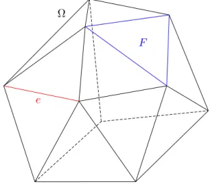
Example 2.6 (Polyhedral Domain) A domain Ω⊆ Rⁿ is called polyhedral if (n= 2) it is a polygon or if (n= 3) ∂Ω is a finite union of polygons (called faces) such that for any faceF ⊆∂Ωand any edgee⊆∂F, there exists another face F⁰⊆∂Ω such that e⊆∂F⁰.

Ω

F

e

Figure 2.1: Example of a polyhedral domain in R³

2.4 Sobolev Spaces

Sobolev spaces are function spaces with certain integrability and differentia- bility properties that allow for an easier analysis than smooth functions. It turns out that these spaces are indispensible in the analysis of the finite element method. In this section we will define various Sobolev spaces which we will need later on.

(15)

2. Preliminaries

2.4.1 Positive Integer Order Sobolev Spaces

Sobolev spaces contain functions which are differentiable in a more general sense, this more general definition let’s us talk about the derivative of functions inL^p-spaces for which point evaluations are not well-defined.

Definition 2.7 (Weak Derivative) (Definition 5.8 in [6]) Let k∈N, α∈N^` for some `≤k and Ω⊆Rⁿ an open set. Let u∈L²(Ω), then u has a weak α-partial derivative if there exists ag∈L²(Ω)such that

ˆ

Ω

u(x)∂^αϕ(x)dx= (−1)^kαk¹ ˆ

Ω

g(x)ϕ(x)dx, ∀ϕ∈C_c^∞(Ω).

Then g is called the weak α-partial derivative of u.

Notation: We denote the weakα-partial derivative of uby ∂^αu.

This notation does not conflict with the notation for regular partial derivatives of differentiable functions. Indeed, ifuhas a regular derivative ∂^αu, then it is also the weakα-partial derivative because the definition of the weak derivative is just the integration by parts formula appliedkαk₁-times.

This generalized definition of partial derivative is crucial for the construction of Sobolev spaces which are an essential tool in the analysis of the finite element method.

Definition 2.8 (Sobolev space of Positive Integer Order) Letk, p∈N, then we define theSobolev space W^k,p(Ω)as

W^k,p(Ω) :={u∈L^p(Ω)| ∀kαk₁ ≤k:∂^αu∈L^p(Ω)}.

The associated norm on this space is defined as

kuk_Wk,p(Ω) :=



 X

kαk₁≤k

k∂^αuk^p_L_p_(Ω)





1/p

, p∈N,

kuk_Wk,∞(Ω):= max

kαk₁≤kk∂^αuk_L∞(Ω), p=∞.

Notation: For p= 2 we write H^k(Ω) :=W^k,2(Ω).

In order to prove properties about functions in Sobolev spaces the following famous theorem by Meyers and Serrin is frequently invoked.

Theorem 2.9 [18] Let Ω be an open set and p < ∞ an integer. Then C^∞(Ω)∩W^k,p(Ω)is dense in W^k,p(Ω).

6

(16)

2.4. Sobolev Spaces More specifically, this means that for anyu∈W^k,p(Ω), there exists a sequence

(un)n inC^∞(Ω)∩W^k,p(Ω) such that

ku_n−uk_Wk,p(Ω)→0, asn→+∞.

The last positive integer order Sobolev space that we we define is a Sobolev space which will be useful when considering Dirichlet boundary value problems where the solution is supposed to vanish on the boundary.

Definition 2.10 Let Ω⊆Rⁿ be open and k, p be non-negative integers. We define the Sobolev space W₀^k(Ω)as

W₀^k,p(Ω) :=C_c^∞(Ω)^k·k^{W k,p(Ω)}.

The intuitive way to think about this space is as a space of functions which

’vanish’ on∂Ω. These functions obviously don’t vanish in the pointwise sense since pointwise values of functions in L^p-spaces aren’t well defined.

2.4.2 Fractional Order Sobolev Spaces

Sobolev spaces of fractional order can be defined in three different ways. The first way is as the closure of a certain space with respect to an appropri- ate norm, the second way is using the Fourier transform and the third way is by using interpolation. All these definitions are equivalent under certain assumptions on the boundary of the domain. We will only use the first definition which uses the so-called Sobolev-Slobodeckij norms which are similar to H¨older norms but integrated. We start by introducing the Sobolev-Slobodeckij (semi)norms.

Definition 2.11 (Sobolev-Slobodeckij (semi)norm) (Page 56 in [19]) Let Ω ⊆ Rⁿ be an open set and s ∈ R⁺, θ ∈ (0,1), p ∈ N such that s =bsc+θ.

Then we define the Sobolev-Slobodeckij seminorm|·|_Ws,p(Ω) as

|u|_Ws,p(Ω) :=

ˆ

Ω

ˆ

Ω

|u(x)−u(y)|^p

|x−y|^θp+n dxdy

!1/p

, ∀u∈C^∞(Ω) and the Sobolev-Slobodeckij norm as

kuk_Ws,p(Ω):=



 X

kαk₁≤bsc

k∂^αuk^p_L_p_(Ω)+ X

kαk₁≤bsc

ˆ

Ω

ˆ

Ω

|∂^αu(x)−∂^αu(y)|^p

|x−y|^θp+n dxdy





1/p

,

=



 X

kαk₁≤bsc

k∂^αuk^p_Lp(Ω)+ X

kαk₁≤bsc

|∂^αu|^p_Ws,p(Ω)





1/p

, ∀u∈C^∞(Ω)

(17)

2. Preliminaries

Now we have the tools to define fractional order Sobolev spaces.

Definition 2.12 (Sobolev Space W^s,p) (Page 56 in [19]) LetΩ⊆Rⁿand s⁺∈R. Then we define the space W^s,p(Ω)as

W^s,p(Ω) :={u∈C^∞(Ω)| kuk_Ws,p(Ω)<+∞}^k·k^{W s,p(Ω)}. We get a similar definition for the spaceW₀^s,p(Ω).

Definition 2.13 Let Ω⊆Rⁿ, s >0 andp a non-negative integer. We define the Sobolev spaceW₀^s(Ω)as

W₀^s,p(Ω) :=C_c^∞(Ω)^k·k^{W s,p(Ω)}.

2.5 Sobolev Spaces on the Boundary

In the following we will need Sobolev spaces for functions defined on the boundary of a bounded domain Ω. These spaces are somewhat harder to define than regular Sobolev spaces because we have to take into account the regularity of the boundary.

Definition 2.14 (Definition 2.4.1 in [19]) LetΩbe a Lipschitz orC^k-domain for some k ≥1 and ` ≤1 for Lipschitz domains and ` ≤k for C^k-domains.

Fix a measurable subset Γ ⊆ Ω. Let {ψ_U : B₂ → U}_U∈_U be the associated bijective mappings from Definition 2.5. For any functionuU :U →R defined on aU ∈U we define uˆU as

ˆ

uU :=uU◦ψU :B₂⁰ →R.

Then we define the Sobolev spaceH^`(Γ) as

H^`(Γ) :={u: Γ→R| ∀U ∈U: ˆuU ∈H₀^`(B₂⁰)}.

Moreover, we equip this space with the norm kuk²_H`(Γ):= X

kαk₁≤`

k∂^αuk²_L2(Γ),

for `∈Nand kuk²_H`(Γ):= X

kαk₁≤b`c

k∂^αuk²_L2(Γ)+ X

kαk₁≤b`c

ˆ

Γ

ˆ

Γ

|∂^αu(x)−∂^αu(y)|²

|x−y|^n−1+2θ ds(x)ds(y), for `∈R\Nwhere θ:=`− b`c and

∂^αu(x) := X

U∈U

∂_ξ^α( ˆu_U)(ξ), 8

(18)

2.5. Sobolev Spaces on the Boundary with x := ψ_U,0(ξ). Here ∂_ξ^α just means differentiation with respect to the

variableξ. The norms above derived is derived from the inner products defined by

hu, vi²_H`(Γ):= X

kαk₁≤b`c

h∂^αu, ∂^αvi²_L2(Γ)

for `∈N and

hu, vi²_H`(Γ):= X

kαk₁≤b`c

h∂^αu, ∂^αvi²_L2(Γ)

+ X

kαk₁≤b`c

ˆ

Γ

ˆ

Γ

|∂^αu(x)−∂^αu(y)||∂^αv(x)−∂^αv(y)|

|x−y|^n−1+2θ ds(x)ds(y), for`∈R\N.

The next Sobolev space is specifically needed because of the fact that extending a function u ∈H^1/2(Γ) for some measurable Γ ⊆∂Ω by 0 onto ∂Ω does not imply that u∈H^1/2(∂Ω).

Definition 2.15 (Lions-Magenes space) (Section 4.1 in [23]) LetΩ⊆Rⁿ be a bounded domain and Γ be a measurable subset of∂Ω. Then we define the Lions-Magenes space as

H₀₀^1/2(Γ) :={u∈L²(Γ)|u˜∈H^1/2(∂Ω)},

where u˜ is the extension by zero of u ∈ L²(Γ) on ∂Ω\Γ. The norm on this space is given by

kuk²

H₀₀^1/2(Γ):=kuk²_L2(∂Ω)+|u|²

H₀₀^1/2(Γ), where

|u|²

H₀₀^1/2(Γ):=|u|²_H1/2(Γ)+ ˆ

Γ

u²(x)

d(x, ∂Γ)ds(x).

This turnsH₀₀^1/2(Γ) into a Hilbert space.

Remark. Usually n= 3, Ω is a polyhedral domain and Γ is one of its faces.

Note that a Hilbert space requires an inner product while we only defined a norm on H₀₀^1/2(Γ). However, the inner product which induces this norm is defined in the obvious way since all norms are just of the L²-kind.

2.5.1 Negative Order Sobolev Spaces

In this section we define Sobolev spaces of negative order which will be denoted byW^−k,p. These are constructed using dual spaces of Banach spaces. For this we first define the dual space.

(19)

2. Preliminaries

Definition 2.16 (Definition 2.53 in [6]) Let X be a Banach space over K=Ror C. The dual space of X is defined as the space

X^∗ :={L∈Hom(X, K)|Lcontinuous}

equipped with the norm

kLk_op := sup

kxk≤1

|L(x)|.

Remark. (X^∗,k·k_op) is again a Banach space.

The only thing we now need is to fix a Banach space which will be the predual of this space. For this we use the spaces W₀^k,p. This leads us to the following to the following definition.

Definition 2.17 (Negative Order Sobolev Space) Let Ω ⊆ Rⁿ and p ∈ Nand k >0. Then we define the Sobolev space W^−k,p(Ω)as

W^−k,p(Ω) :=W₀^k,p(Ω)^∗.

Remark. If Γ⊆Rⁿ is a closedC^k-surface, then it has no boundary. Hence H₀^`(Γ) =H^`(Γ), ∀`≤k.

Therefore we have

H^−`(Γ) =H^`(Γ)^∗.

Moreover, we have anL²-dual pairing betweenH^−`(Γ) andH^`(Γ) given by H^−`(Γ)×H^`(Γ)→K : (u, v)7→ h˜u, vi_H`(Γ),

where ˜u is the unique element of H^`(Γ) which corresponds to u under the Fr´echet-Riesz representation theorem (Corollary 3.19 in [6]).

Definition 2.18 (Dual Sobolev Norms) Let Ω ⊆ Rⁿ be a bounded Lips- chitz or C^k-domain and consider the Sobolev space H^−`(∂Ω) for some `≤k.

We define a norm on this space by setting kuk_H−`(∂Ω) :=kuk_op,

as usual for the dual space of a Banach space. Because of theL²-dual pairing betweenH^`(∂Ω) and H^−`(∂Ω) we can rewrite this as

kuk_H−`(∂Ω)= sup

06=v∈H^`(∂Ω)

|h˜u, vi_H`(∂Ω)| kvk_H`(∂Ω)

,

where u˜ is the unique element of H^`(Γ) which corresponds to u under the Fr´echet-Riesz representation theorem (Corollary 3.19 in [6]).

10

(20)

2.5. Sobolev Spaces on the Boundary

2.5.2 Sobolev Spaces H(curl; Ω), H₀(curl; Ω) and H^δ(curl; Ω) One application of the edge and face lemma is in the numerical simulation of Maxwell’s equation. For the analysis of these methods we need certain vectorial Sobolev spaces which we introduce in the next couple of sections. For the weak formulation of Maxwell’s equations we need Sobolev spaces involving the curl operator.

Definition 2.19 (Sobolev Space H(curl; Ω)) (A.5.3 in [21]) Let Ω⊆R³ be a Lipschitz domain. The Sobolev spaceH(curl; Ω) is defined as

H(curl; Ω) :={u∈(L²(Ω))³|curl u∈(L²(Ω))³}, equipped with the inner product

hu,vi_H(curl;Ω)=hu,vi_(L2(Ω))³+hcurl u,curl vi_(L2(Ω))³, ∀u,v∈H(curl; Ω).

To define the Sobolev spaceH₀(curl; Ω), we need a trace theorem which allows us to define the tangential component of a function u∈H(curl; Ω).

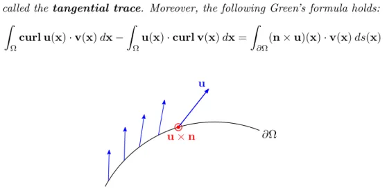
Lemma 2.20 (Tangential Trace) (Lemma A.22 in [21]) Let Ω⊆ R³ be a Lipschitz domain with unit outward normal n. Then the operator

γt: (C^∞(Ω))³→(C^∞(∂Ω))³ :u7→u×n, can be extended to a bounded operator

γt:H(curl; Ω)→(H^−1/2(∂Ω))³,

called the tangential trace. Moreover, the following Green’s formula holds:

ˆ

Ω

curl u(x)·v(x)dx− ˆ

Ω

u(x)·curl v(x)dx= ˆ

∂Ω

(n×u)(x)·v(x)ds(x)

u×n u

∂Ω

Figure 2.2: Example of a smooth vector field u together with its tangential trace u×n at a single point

(21)

2. Preliminaries

Definition 2.21 (Sobolev Space H₀(curl; Ω)) (A.5.3 in [21]) Let Ω ⊆ R³ be a Lipschitz domain. The Sobolev spaceH0(curl; Ω) is defined as

H₀(curl; Ω) :={u∈H(curl; Ω)|γ_tu= 0}.

Definition 2.22 (Sobolev Space H^δ(curl; Ω)) (Section 2 in [15]) Let Ω be a Lipschitz domain and δ > 0 fixed. Then we defined the Sobolev space H^δ(curl; Ω) as

H^δ(curl; Ω) :={v∈(H^δ(Ω))³ |curl v∈(H^δ(Ω))³}, equipped with the norm

kvk²_Hδ(curl;Ω):=kvk²_HδΩ)+kcurl vk²_HδΩ).

SoH^δ(curl; Ω) is just a fractional order analogue ofH^δ(Ω) for theH(curl; Ω) Sobolev spaces.

2.5.3 Sobolev Spaces H(div; Ω), H₀(div; Ω) and H₀(div₀; Ω)

In this section we define Sobolev spaces involving the divergence operator.

The definitions are similar to those for the H(curl,Ω) spaces defined in the previous section but in this case for the divergence operator.

Definition 2.23 (Sobolev Space H(div; Ω)) (A.5.1 in [21]) Let Ω⊆ R³ be a Lipschitz domain. We define the Sobolev spaceH(div; Ω) as

H(div; Ω) :={u∈(L²(Ω))³|divu∈L²(Ω)}, equipped with the inner product

hu,vi_H_(div;Ω):=hu,vi²_(L2(Ω))³ +hdivu,divvi²_L2(Ω), ∀u,v∈H(div; Ω).

Next we need a lemma similar to Lemma 2.20, but for the normal component of functions inH(div ; Ω).

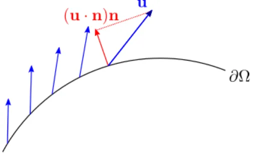
Lemma 2.24 (Normal Trace) (Lemma A.19 in[21]) Let Ω be a Lipschitz domain with unit outward normaln. Then the operator

γn: (C^∞(Ω))³→C^∞(∂Ω) :u→u·n, can be extended to a bounded operator

γ_n:H(div; Ω)→H^−1/2(∂Ω), called the normal trace.

12

(22)

2.6. The Dirichlet Trace

(u·n)n u

∂Ω

Figure 2.3: Example of a smooth vector fieldutogether with its normal trace u·n at a single point

Now that we know that the normal component for functions in H(div; Ω) is well-defined, we proceed with defining two other similar Sobolev spaces.

Definition 2.25 (Sobolev Spaces H₀(div; Ω) and H₀(div₀; Ω)) (A.5.1 in [21]) Let Ω ⊆ R³ be a Lipschitz domain. We define the Sobolev space H₀(div; Ω) as the subspace of H₀(div; Ω) defined as

H₀(div; Ω) :={u∈H(div; Ω)|γ_nu= 0}

and the Sobolev space H₀(div₀; Ω) as the subspace of H₀(div; Ω) defined as H0(div0; Ω) :={u∈H0(div; Ω)|divu= 0}.

2.6 The Dirichlet Trace

Consider the following Dirichlet boundary condition:

u=f, on ∂Ω,

for some f : ∂Ω → R. If u is a strong solution to a PDE, then it is at least continuous and therefore the interpretation of the Dirichlet boundary condition is evident. On the boundary of Ω we have pointwise equality

u(x) =f(x), ∀x∈∂Ω.

However, when considering weak solutions to a PDE, these will generally be elements of a certain Sobolev space. In general, pointwise evaluation of a function in an L^p-space is not well defined. Therefore we need to generalize what it means to evaluate a function or more generally to restrict a function to a subset of measure 0 (for example∂Ω). The way this will be done is by extending the operator which assigns to a continuous function u its restriction u|_∂Ω to the boundary of Ω. This generalization will be sufficient for our purposes since Dirichlet boundary conditions are only prescribed on the boundary of the domain of interest.

(23)

2. Preliminaries

Theorem 2.26 (Dirichlet Trace for H¹) (Theorem 4.1 in [23]) Let Ω be a Lipschitz domain. Then there exists a surjective bounded linear operator

γ0:H¹(Ω)→H^1/2(∂Ω), such that

γ0u=u|_∂Ω, ∀u∈H¹(Ω)∩C¹(Ω), and

|γ₀u|_H1/2(∂Ω)≤C|v|_H1(Ω), ∀u∈H¹(Ω)

for some constantC >0. Moreover,γ₀has a right-continuous bounded inverse E:H^1/2(Ω)→H¹(Ω)such that

|Ev|_H1(Ω) ≤C|v|˜ _H1/2(∂Ω), ∀v∈H^1/2(Ω), for some constant C >˜ 0.

14

(24)

Chapter 3 The Finite Element Method

The finite element method is a numerical method for approximating solutions to PDEs. The special approach that the finite element method takes is that it approximates solutions to the variational form of the PDE and not the strong form. Therefore we commence by deriving the variational formulation of a model PDE followed by the general definition of a variational problem.

3.1 Variational Problems

Let us start with an example to illustrate why we’re concerned with variational problems. Consider the following Dirichlet boundary value problem:

(−∆u=f, in Ω,

u= 0, on ∂Ω, (3.1)

for some bounded domain Ω⊆Rⁿ. If we want to find a weak solutionuin some L^p-space, then pointwise values ofu aren’t necessarily well-defined. However, we know that integrals of u can be defined. Let us therefore integrate the above PDE, but we must take care because ∆u is not necessarily integrable.

Therefore we first multiply the PDE by a test functionϕ∈C_c^∞(Ω) and then integrate. This gives

ˆ

Ω

−∆u(x)ϕ(x)dx= ˆ

Ω

f(x)ϕ(x)dx.

Next we apply integration by parts to the left-hand side:

ˆ

Ω

∇u(x)· ∇ϕ(x)dx= ˆ

Ω

f(x)ϕ(x)dx.

Since this holds for all ϕ ∈ C_c^∞(Ω) we get the following equation which we call the variational form of (3.1):

ˆ

Ω

∇u(x)· ∇ϕ(x)dx= ˆ

Ω

f(x)ϕ(x)dx, ∀ϕ∈H₀¹(Ω), (3.2)

(25)

3. The Finite Element Method

by density ofC_c^∞(Ω) inH₀¹(Ω) with respect tok·k_H1(Ω). The reason why we take this norm is because (3.1) only requiresu to have (weak) derivatives up to order one. Notice that the boundary condition for the Dirichlet problem is incorporated in the Sobolev space H₀¹(Ω) of test functions. If we now set V :=H₀¹(Ω) and define the bilinear formaas

a:V ×V →R: (u, v)7→

ˆ

Ω

∇u(x)· ∇v(x)dx, then we can reformulate (3.1) as

a(u, v) =hu, fi_L2(Ω), ∀v∈V.

This last form is what we will abstractly deal with when talking about the finite element method.

3.2 Symmetric and Nonsymmetric Variational Problems

The finite element method approximates solutions to symmetric and nonsymmetric variational problems. In this section we abstractly define what these problems are.

Definition 3.1 (Symmetric Variational Problem) (Page 57 in [3]) Let (H,h·,·iH) be a Hilbert space over K=Ror C,V ⊆ H a closed subspace and a:V ×V → K a bounded, symmetric and coercive bilinear form. Then the associated symmetric variational problem is given by:

GivenF ∈V^∗, findu∈V such that

a(u, v) =F(v), ∀v∈V.

Remark. The nonsymmetric variational problem is similar to the symmetric one with one difference,ais not necessarily symmetric. Moreover, the conditions that ais coercive and bounded is not necessary to define a variational problem. However, we will always assume that these are fulfilled to guarantee the existence of solution for a symmetric variational problem and hence add them to the definition of a variational problem.

We can rewrite a variational problem in a more compact way by introducing an operator associated to the bilinear forma. The existence and unicity of this operator is guaranteed by the Fr´echet-Riesz representation theorem (Corollary 3.19 in [6]).

Definition 3.2 let a a bilinear form as in Definition 3.1. The operator A : V →V associated to a is defined as the unique bounded operator such that

hAu, vi_H =a(u, v), ∀u, v∈V.

16

(26)

3.3. The Finite Element Method Using the above definition, we can rewrite the variational problem from Defi-

nition 3.1 as:

Given f ∈V, findu∈V such that

Au=f, wheref ∈V is the unique element such that

F(v) =hf, vi_H, ∀v∈V.

Again, the existence and unicity off is guaranteed by the Fr´echet-Riesz representation theorem (Corollary 3.19 in [6]).

3.3 The Finite Element Method

Now we can describe how the finite element method works. Given the variational problem: Given F ∈V^∗, find u∈V such that

a(u, v) =F(v), ∀v∈V.

Under the assumption that this is the weak form of some PDE, the finite element method constructs an approximation of the solution u from some finite-dimensional subspace S⊆V. The choice of approximand from this subspace will be an optimal approximation (to be made precise) to the solution of the weak form of the PDE. We start by explaining how the finite-dimensional space S is constructed. The essential ingredient is the mesh which is chosen on the domain where the PDE is defined.

3.4 Meshes and Regularity

The finite dimensional space S is constructed by first considering a mesh on the domain on which the PDE is defined. Let Ω⊆Rⁿbe bounded any domain.

We first define precisely what a mesh is.

Definition 3.3 (Mesh) (Definition 4.2.1 in [10]) A mesh (or triangula- tion)on a bounded domainΩ⊆Rⁿ, n= 2,3, is a finite familyM={K_i}^M_i=1, M ∈ N, of open non-degenerate (curvilinear) polygons (n = 2) or polyhedra (n= 3)such that

1. Ω =

M

[

i=1

K_i

2. ∀i6=j:K_i∩K_j =∅,

3. ∀i6=j :K_i∩K_j is either the empty set, a vertex, an edge or a face of both K_i and K_j.

(27)

We will denote by N(M) the set nodes of the mesh M.

Our results will crucially depend on certain assumptions regarding such a mesh. The two assumptions which we will frequently use are shape regularity and quasi-uniformity. Before giving these definitions we will fix some notation.

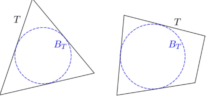
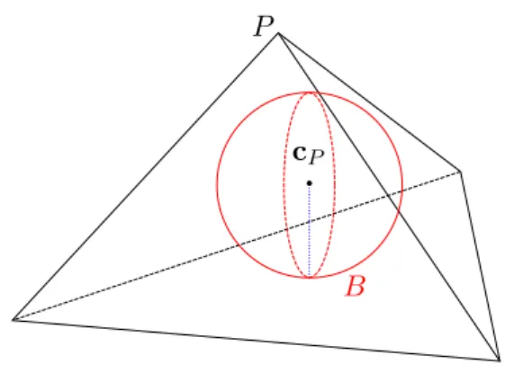
Definition 3.4 (Inscribed Ball) Let T ⊆ Rⁿ, n ∈ N be an open set with compact closure and piecewise smooth boundary. We denote byBT the largest ball contained inT such thatT is star-shaped with respect to B_T.

BT BT

T T

Figure 3.1: Example of the inscribed ball (disk) as in Definition 3.4 Now we are set to give one of the most crucial definitions which is indispensable in the proofs that we will give.

Definition 3.5 (Definition 4.4.13 in [3]) Fix a bounded domainΩ⊆Rⁿ, n= 2,3, and a family of subdivisions {T^h}_0<h≤1 such that

h= max_T_∈T^hdiamT diam Ω ,

i.e. h is the mesh width scaled by 1/diam Ω. The family {T^h}_0<h≤1 is quasi-uniformif there exists a ρ >0 such that

min

T∈T^hdiamBT ≥ρhdiam Ω,

for all h∈(0,1]. The family{T^h}0<h≤1 isnon-degenerateor shape regu- larif there exists a ρ >0 such that for all T ∈ T^h and h∈(0,1]:

diamB_T ≥ρdiamT.

Remark. Notice that the condition for shape regularity is equivalent to the condition

inf

T∈T^h,h∈(0,1]

diamBT

diamT ≥ρ, 18

(28)

3.5. Mesh Refinement Which means we can find for any elementTin the family of meshes{T^h}_0<h≤1,

a ball BT inscribed in T, such thatBT is star-shaped with respect toT such that the size of the ballB_T relative to the size ofT is bounded by some uniform constantρ >0. We also remark that the interval (0,1] is not essential to the definition. Any set H ⊆(0,+∞) can be chosen instead.

3.5 Mesh Refinement

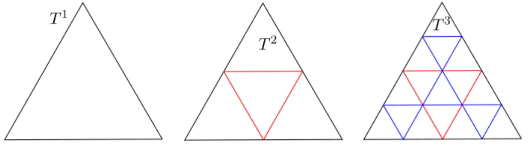
In the last part of this section we describe what kind of mesh refinement we will consider. For our results, we will only consider meshes of triangles and tetrahedrons and therefore will only discuss mesh refinement for these cases. We will describe in detail how regular mesh refinement is done for two dimensional meshes of triangles which result in families of quasi-uniform meshes. A similar (but albeit more complicated) construction can be made for tetrahedral meshes. A graphical illustration of two consecutive refinements is given in Figure 3.2.

T¹

T²

T³

Figure 3.2: Example of midpoint refinement of a triangle

Consider the triangle on the left. This can be thought of as one triangle in a mesh of triangles covering a two dimensional domain. The regular mesh refinement that we will consider is midpoint refinement which goes as follows.

The mesh is locally refined inside each triangle of the mesh, this means that the refinement of the mesh inside one triangle is independent of what happens for a different triangle. Therefore we illustrate this only with one triangle.

The refinement is constructed by connecting the midpoints of each edge of the triangle. This results in the middle triangle in Figure 3.2 which now consists of four smaller triangles. The next refinement is done in exactly the same way by connecting the midpoints of the edges of each triangle with each other. The result of this is shown in the right triangle in Figure 3.2. When we talk about a family of quasi-uniform meshes, we will assume that they are the result of such a refinement.

(29)

3.5.1 Finite Elements and Local Shape Functions

Now that we have a mesh on our domain, we can construct the finite-dimensional space of functionsS which we talked about before. This is done by choosing a basis for the functions defined on each element of the mesh separately. This results in the following definition.

Definition 3.6 (Finite Element) (Definition 3.3.1 in [3]) A finite element is a triple (K,P_K,N_K) where

1. K⊆Rⁿis an open set with compact closure and piecewise smooth boundary (element domain),

2. P_K is a finite-dimensional space of functions onK (local shape functions),

3. N_K ⊆ P_K^∗ is a basis for P_K^∗ (nodal variables/degrees of freedom).

Let us illustrate this concept with an easy example.

Example 3.7 (Linear Lagrangian Finite Elements in 2D) (Example 3.2.1 in [3]) Let K ⊆R² be a triangle and set

P_K :={x∈K 7→a^Tx+b|a∈Rⁿ, b∈R}.

If we define N_K as

N_K :={ev₁,ev₂,ev₃} ⊆ P_K^∗,

which are the point evaluations at the three vertices of the triangle, then (K,P_K,N) is a finite element. Indeed, N_K is the dual basis associated to the barycentric coordinate functions {λ₁, λ₂, λ₃} with respect to the nodes of the triangle. See Figure 3.3 for an illustration of these functions.

λ1

λ₂

λ₃ 1

1

1 K

Figure 3.3: The barycentric coordinate functions associated to the triangleK The main idea of the finite element method is to approximate the solution of a PDE on each elementK by a linear combination of functions inP_K. Before we discuss the global finite-dimensional spaceS we discuss a special case where each element is related to one another.

20

(30)

3.5. Mesh Refinement 3.5.2 Affine equivalence

We will be interested in a special type of finite element. Namely, the ones which are all just transformations of one single element in the mesh. By this we mean that after fixing a single finite element in the given mesh, all the other finite elements are just transformations of this one element.

Definition 3.8 (Affine Equivalence) (Definition 3.4.1 in [3]) Let(K,P,N) be a finite element with K ⊆Rⁿ and let F :Rⁿ → Rⁿ be an invertible affine map. The finite element ( ˆK,Pˆ,Nˆ) is affine equivalent to(K,P,N) if

1. F(K) = ˆK, 2. F^∗Pˆ=P, 3. F∗N = ˆN.

Here F^∗ is the pullback of F, defined by

F^∗( ˆf) := ˆf◦F, ∀fˆ∈P,ˆ and F∗ is thepushforward of F, defined by

(F∗N)( ˆf) :=N(F^∗( ˆf)), ∀N ∈ N,fˆ∈Pˆ.

3.5.3 Global Shape Functions and piece-wise polynomial spaces In the previous section we introduced the notion of local shape functions.

These are functions defined locally on an element domain. To obtain an approximation to a solution of a PDE we need a function defined on the en- tire domain we’re considering. These globally defined functions will be called (global) shape functions. There is no single definition of global shape functions since the properties of the global shape functions differ depending on the function space setting. Some examples of these properties are global continuity, continuity of the tangential or normal components etc.

To illustrate this concept we give an example. A commonly used choice of local shape functions are polynomials of a certain degree. If (piece-wise) polynomials are used as shape functions, then the name Lagrangian finite element method is used as in Example 3.7. It is this finite element method in which we are interested. First we need to introduce the concept of polynomial spaces.

Definition 3.9 (Polynomial spaces) (Definition 4.2.2 in [10]) Let K ⊆ Rⁿ be a set (we don’t require any regularity). We define the set ofpolynomi- als of degree p∈N on K as

P_p(K) :=







q ∈C(K)

∃(a_α)kαk₁≤p ⊆R:∀x∈K:q(x) = X

kαk₁≤p

aαx^α





 .

(31)

So P_p(K) is the space of multivariate polynomials in n variables on K such that the (total) degree is at most p.

Remark. In the above definition, the α ∈ N0. Therefore the sum in the definition is always finite and hence well-defined.

Now that we have defined polynomial spaces, we can define the relevant space of global shape functions which will be a piece-wise polynomial space. As we will see, this function space will locally be a polynomial space.

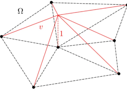
Definition 3.10 (Lagrangian Shape Functions) (Definition 4.3.1 in [10]) Let Ω ⊆ Rⁿ be a Lipschitz domain equipped with a simplicial mesh M and p ∈ N. The space of p-th degree Lagrangian global shape functions is defined as

S_p⁰(M) :={v∈C(Ω)| ∀K∈ M:v|_K ∈ P_p(K)}.

We denote by S_p,0⁰ (M) the subspace of functions in S_p⁰(M) that vanish on∂Ω, i.e.

S_p,0⁰ (M) :={v∈ S_p⁰(M)|v|_∂Ω= 0}.

Last, for anyΩ⁰⊆Ω, we defineS_p⁰(M|_Ω⁰)as the p-th degree Lagrangian global shape functions with repect to the mesh onΩ⁰ induced by T^h.

v 1

Ω

Figure 3.4: Example of a Lagrangian global shape functionv which is a basis function forS_p⁰(M) whereMis the mesh on Ω

Remark. If the mesh is just a grid (a Cartesian product of 1-dimensional meshes), then the above definition of the Lagrangian shape functions simplifies.

Indeed, we can replace P_p(K) by the space of tensor product polynomials P_p^⊗(K) which is defined as

P_p^⊗(K) :=

(

q∈ P_p(K)

∃p₁, . . . , pn∈ P_p(K) :∀x∈K:q(x) =

n

Y

k=1

p_k(x_k) )

.

22

(32)

3.5. Mesh Refinement 3.5.4 Ritz-Galerkin Approximation

Now that we have defined the finite-dimensional space of approximands with respect to a given mesh we explain in what way an approximation is constructed to the solution of a PDE. The finite element method approximates the solution of a PDE on each element by the Ritz-Galerkin method. This method is surprisingly simple and elegant to describe. We state it in the following definition.

Definition 3.11 (Ritz-Galerkin Approximation Problem) (Section 0.2 in [3]) Let H be a Hilbert space overK(=R or C), V ⊆ H a closed subspace and a : V ×V → K a bounded and coercive bilinear form. Consider the symmetric variational problem: Given F ∈V^∗, find u∈V such that

a(u, v) =F(v), ∀v ∈V.

Now fix a finite-dimensional subspace V^h ⊆ V. Then the associated Ritz- Galerkin approximation problem is defined as: Findu^h∈V^h such that

a(u^h, v^h) =F(v^h), ∀v^h∈V^h.

So the Ritz-Galerkin approximation problem associated to a symmetric variational problem is just that same variational problem with a smaller solution space, i.e. the restriction of V to some finite dimensional subspace.

Remark 3.12 The Ritz-Galerkin approximation problem for a nonsymmetric variational problem is defined in exactly the same way as for the symmetric case.

We end this section by describing the philosophy of the finite element method in a bit more detail since we now have defined all the relevant concepts. Given a variational problem (resulting from a PDE), a mesh is chosen on the domain Ω. On each element domain, suitable local shape functions and nodal variables are chosen. Then the solution to the variational problem is approximated by computing the solution to the associated Ritz-Galerkin approximation problem which boils down to solving a system of linear equations (since it is a linear equation on a finite-dimensional vector space).

(33)

(34)

Chapter 4 Inverse Inequalities

In this chapter we are concerned with inverse inequalities (also called inverse estimates). These inequalities will be indispensable when we prove the edge and face lemma. Let us first clarify the term inverse inequality and motivate why such inequalities exist.

Consider for example the spaces W^k,p(Ω), k ∈ N, for some bounded domain Ω⊆Rⁿ and p∈N. Then we have the obvious continuous embeddings

W^1,p(Ω),→W^2,p(Ω),→. . . ,→W^k,p(Ω),→W^k+1,p(Ω),→. . . . (4.1) Moreover it is obvious that there are no embeddings

L^∞(Ω),→W^k,p(Ω), L^p(Ω),→W^k,p(Ω). (4.2) However, for finite element spaces certain converses of (4.1) are true. Even (4.2) turns out to be true for certain finite element spaces. This is not very surprising because of norm equivalence on finite dimensional normed spaces.

Therefore, any two well-defined norms on a finite element space are related by two-sided inequalities. The nontrivial inequalities of this kind are inverse inequalities. So why are we interested in these inequalities if norm equivalence already tells us that these two-sided inequalities exist? The essential part here is that we want to state these inequalities with an explicit dependence on h, i.e. as an inequality of the form

ku^hk_Wk,p(Ω)≤Cb(h)ku^hk_W`,q(Ω),

for some constant C > 0 (independent of u^h and h) and k > `or k= `and p > q, whereb:R⁺→ Ris some function and ` < k. Here u^h is an arbitrary finite element function on some domain Ω ⊆ Rⁿ with respect to a mesh T^h with mesh widthh >0. For the sake of argument assume that all norms are well defined.

(35)

4. Inverse Inequalities

These inequalities are essential for error analysis and for constructing preconditioners for the linear systems resulting from Galerkin discretization. In this section we will state and prove certain inverse inequalities which we will need in the proofs of the edge and face lemma.

Before continuing, we fix some notation that will be used in the proofs from now on. The the symbols.,&,=

∼ will be frequently used , but never in the statements of the results. The interpretation is as follows, let y1, y2 be two quantities of interest. We write y₁ . y₂ if there exists a constant C > 0 independent of the mesh parameters such thaty1.y2. The interpretation of

&is analogous. We say y1=

∼ y2 if both y1.y2 and y1 &y2.

4.1 Discrete variants

This section is devoted to introducing some concepts which will be needed to help prove the inverse inequalities that will be stated in this section. This will mostly consist of generalizing known concepts like harmonic functions to the discrete setting of finite element spaces.

4.1.1 Scott-Zhang Quasi-Interpolant

In contrast to the nodal value interpolant which just interpolates a continuous function on the nodes of the mesh, the average nodal value interpolant is used to interpolate possibly discontinuous functions.

Definition 4.1 (Scott-Zhang Quasi-Interpolant) (Section 4.2.1 in [23]) Let Ω⊆ Rⁿ be a polyhedral domain equipped with a mesh T^h. Let T_k be an (n−1)-simplex from the mesh T^h with vertices{z_k}ⁿ_k=1 such thatz1=zk for any z_k ∈ N(T^h) =: {z₁, . . . ,z_N_h}. Let θ_k ∈ P₁(T_k) be the unique function

such that ˆ

Tk

θ_k(x)λ_k(x)dx=δ_k1, k= 1, . . . , n,

where λ_k is the barycentric coordinate of T_k with respect to z_k. The Scott- Zhang quasi-interpolantΠh :H¹(Ω)→ S₁⁰(T^h) is defined as

(Π_hv)(x) :=

Nh

X

k=1

ϕ_k(x) ˆ

Tk

θ_k(ξ)v(ξ)dξ, ∀x∈Ω,

where (ϕ_k)^N_k=1^h is the nodal basis for S₁⁰(T^h).

Remark. The choice of Tk is not unique in general, but if xk ∈ ∂Ω, then we can choose T_k such that T_k ⊆ ∂Ω. For an illustration of this, we refer to Figure 4.1.

26

(36)

4.1. Discrete variants

∂Ω

T_k z1 = ˜z1 =x_k

T˜k

z2

z₃ = ˜z₃

˜z2

Figure 4.1: Example of two possibilities T_k and ˜T_k of (n−1)-simplices associated to the node xk. Sincexk∈∂Ω, the choice of (n−1)-simplex can indeed be chosen to in ∂Ω.

It turns out that the Scott-Zhang quasi-interpolant Π_h is not only a bounded operator, but also that the family {Π_h} forms an equicontinuous family of operators. This is stated in the following lemma.

Lemma 4.2 [20] LetΠ_h be the Scott-Zhang quasi-interpolant as in Definition 4.1. Then

kΠ_hvk_H1(Ω) ≤C₁kvk_H1(Ω), ∀v∈H¹(Ω),

|Π_hv|_H1(Ω) ≤C2|v|_H1(Ω), ∀v∈H¹(Ω),

where the constants C₁ and C₂ are independent of h and depend only on the shape regularity of the mesh.

4.1.2 The (Generalized) Discrete Harmonic Extension

Consider a polyhedral domain Ω ⊆ Rⁿ, n = 2,3 equipped with a mesh T^h with mesh widthh > 0. Fix a function u ∈C(∂Ω). The harmonic extension of uinto Ω is defined as the solution to the Dirichlet boundary value problem

(−∆˜u= 0, in Ω,

˜

u=u, on∂Ω.

(37)

4. Inverse Inequalities

We want to generalize this concept of harmonic extension to piece-wise linear and globally continuous functions. We start by looking at the variational form of this PDE as we did in the beginning of Chapter 3. The same computation gives us the following variational formulation

ˆ

Ω

∇˜u(x)· ∇v(x)dx= 0, ∀˜u, v∈H₀¹(Ω).

Since we don’t want to look at the values on the boundary, we takeH₀¹(Ω) as the space of test functions. Imposing the correct boundary values gives us a generalization of harmonic extensions, but this isn’t enough. Finite element functions which vanish at the boundary don’t live in the whole space H₀¹(Ω) since they form only a finite dimensional subspace of this Sobolev space. There- fore we should take S_1,0⁰ (T^h) as the space of test functions. This motivates the following definition.

Definition 4.3 (Discrete Harmonic Extension) (Section 4.2.2 in [23]) Let Ω ⊆ Rⁿ be a polyhedral domain equipped with a quasi-uniform of family of meshes {T^h}. Fix a u ∈ S₁⁰(T^h|_∂Ω), the discrete harmonic extension of u into Ωis defined as the solution u^h∈ S₁⁰(T^h) of the variational problem

ˆ

Ω

∇u^h(x)· ∇v^h(x)dx= 0, ∀v^h ∈ S_1,0⁰ (T^h).

u^h =u, on ∂Ω.

This definition is further generalized by considering the H¹-inner product instead of theH¹-pseudo-inner product.

Definition 4.4 (Generalized Discrete Harmonic Extension) (Section 4.2.2 in [23]) Let Ω ⊆ Rⁿ be a polyhedral domain equipped with a quasi-uniform family of meshes {T^h}. Fix a u ∈ S₁⁰(T^h|_∂Ω), we define the generalized discrete harmonic extension of u into Ω as the solution u^h ∈ S₁⁰(T^h) of the variational problem

hu^h, v^hi_H1(Ω) = 0, ∀v^h∈ S_1,0⁰ (T^h).

u^h =u, on ∂Ω.

Remark. Any function u ∈ S₁⁰(T^h) satisfying the definition of the (generalized) discrete harmonic extension is called a (generalized) discrete harmonic function.

The crucial property of these harmonic extensions is stated and proved in the following proposition. As we can intuitively expect, a discrete harmonic function can be controlled in a certain sense by its values on the boundary.

28