The Spectral-Element Method

(1)

Heiner Igel

Department of Earth and Environmental Sciences Ludwig-Maximilians-University Munich

(2)

Outline

1 Introduction Motivation History

Spectral Elements in a Nutshell

2 Weak Form of the Elastic Equation Weak Forms

Global system Solution scheme

3 Getting Down to the Element Level Interpolation with Lagrange Polynomials

Numerical Integration: The Gauss-Lobatto-Legendre Approach Derivatives of the Lagrange Polynomials

4 Global Assembly and Solution

(3)

Introduction Motivation

Motivtion

High accuracy for wave propagation problems Flexibility with Earth model geometries

Accurate implementation of boundary conditions Efficient parallelization possible

(4)

History

Originated in fluid dynamics (Patera, 1984, Maday and Patera, 1989)

First applications to seismic wave propagation by Priolo, Carcione and Seriani, 1994)

Initial concepts around Chebyshev polynomials (Faccioli, Maggio, Quarteroni and Tagliani, 1996)

Use of Lagrange polynomials (diagonal mass matrix) by Komatitsch and Vilotte (1998)

Application to spherical geometry using the cubed sphere concept (Chaljub and Vilotte, 2004)

Spectral elements in spherical coordinates by Fichtner et al. (2009)

Community code "specfem" widely used for simulaton and inversion (e.g., Peter et al. 2011).

(5)

Introduction History

History

Community code "specfem" widely used for simulaton and inversion (e.g., Peter

(6)

History

(7)

History

(8)

History

(9)

History

(10)

History

(11)

Specfem 3D

Logo of the wellknown community code with a snapshot of global wave propagation for a simulation of the devastating M9.1 earthquake near Sumatra in December, 2004.

The open-source code is hosted by the CIG project

(www.geodynamics.org).

(12)

Spectral Elements in a Nutshell

Snapshot of the displacement fielduduring a simulation in a strongly heterogeneous medium.

Zoom into the displacement field inside an element discretised with order N=5 collocation points

Exact interpolate using Lagrange polynomials.

Gauss-Lobatto-Legendre Numerical integration scheme.

(13)

Introduction Spectral Elements in a Nutshell

1-D elastic wave equation

ρ(x)¨u(x,t) =∂x[µ(x)∂xu(x,t)] + f(x,t)

udisplacement f external force ρmass density µshear modulus

(14)

Boundary condition

No traction perpendicular to the Earth’s free surface σ_ij n_j =0

normal vectorn_j,σij is the symmetric stress tensor µ∂_xu(x,t)|_x=0,L=0

where our spatial boundaries are atx =0,Land the stress-free condition applies at both ends

(15)

Introduction Spectral Elements in a Nutshell

Spectral Element: Essentials

Weak formulation of the wave equation

Transformation to the elemental level (Jacobian)

Approximation of unknown functionuusing Lagrange polynomials Evaluation of the 1st derivatives of the Lagrange polynomials Numerical integration scheme based on GLL quadrature Calculation of system matrices at elemental level

Assembly of global system of equations

Extrapolation in time using a simple finite-difference scheme

(16)

Weak Form of the Elastic Equation

(17)

Weak Form of the Elastic Equation Weak Forms

Galerkin Principle

The underlying principle of the finite-element method

Developed in context with structural engineering (Boris Galerkin, 1871-1945)

Also developed by Walther Ritz (1909) - variational principle Conversion of a continuous operator problem (such as a differential equation) to a discrete problem

Constraints on a finite set of basis functions

(18)

Weak Formulations

Multiplication of pde with test functionw(x)on both sides.

G is here the complete computational domain defined with x ∈G= [0,L].

Z

G

w ρu¨ dx − Z

G

w ∂x (µ ∂xu)dx = Z

G

w f dx

(19)

Weak Form of the Elastic Equation Weak Forms

Integration by parts

Z

G

w ρu¨dx + Z

G

µ ∂xw ∂x udx = Z

G

w f dx

where we made use of the boundary condition

∂xu(x,t)|_x=0=∂xu(x,t)|_x=L=0

(20)

The approximate displacement field u(x,t) ≈ u(x,t) =

n

X

i=1

u_i(t)ψi(x).

Discretization of space introduced with this step Specific basis function not yet specified

In principle basis functions defined on entire domain (-> PS method)

Locality of basis functions lead to finite-element type method

(21)

Weak Form of the Elastic Equation Global system

Global system after discretization

Use approximation ofuin weak form and (!) use the same basis function as test function

Z

G

ψiρudx¨ + Z

G

µ∂xψi∂xudx = Z

G

ψifdx

with the requirement that the medium is at rest a t=0.

(22)

Including the function approximation for u(x,t)

... leads to an equation for the unknown coefficientsu_i(t)

n

X

i=1

¨u_i(t) Z

Ge

ρ(x)ψj(x)ψi(x)dx

+

n

X

i=1

u_i(t)

Z

Ge

µ(x)∂xψ_j(x)∂xψ_i(x)dx

= Z

G

ψ_i f(x,t)dx

for all basis functionsψ_j withj =1, ...,n. This is the classical algebro-differential equation forfinite-elementtype problems.

(23)

Matrix notation

This system of equations with the coefficients of the basis functions (meaning?!) as unknowns can be written in matrix notation

M·u(t) +¨ K·u(t) =f(t)

MMass matrix KStiffness matrix

terminology originates from structural engineering problems

(24)

Matrix system graphically

The figure gives an actual graphical representation of the matrices for our 1D problem.

The unknown vector of coefficientsuis found by a simple

finite-difference procedure. The solution requires the inversion of mass

(25)

Mass and stiffness matrix

Definition of the - at this point - global mass matrix M_ji =

Z

G

ρ(x)ψ_j(x)ψ_i(x)dx

and the stiffness matrix K_ji =

Z

G

and the vector containing the volumetric forcesf(x,t)

(26)

Mapping

A simple centred finite-difference approximation of the 2nd derivative and the following mapping

u^new → u(t+dt) u → u(t) u^old → u(t−dt)

leads us to the solution for the coefficient vectoru(t+dt)for the next time step as already well known from the other solution schemes in previous schemes.

(27)

Weak Form of the Elastic Equation Solution scheme

Solution scheme

u^new =dt² h

M⁻¹(f−K u)i

+2u −u^old

General solution scheme for finite-element method (wave propagation)

Independent of choice of basis functions Mass matrix needs to be inverted!

To Do: good choice of basis function, integration scheme for

(28)

Getting Down to the Element Level

(29)

Getting Down to the Element Level

Element level

(30)

System at element level

n

X

i=1





¨u_i(t)

ne

X

e=1

Z

Ge

ρ(x)ψ_j(x)ψ_i(x)dx







+

n

X

i=1





u_i(t)

ne

X

e=1

Z

Ge







=

ne

X

e=1

Z

Ge

ψ_j(x)f(x,t)dx .

(31)

Local basis functions

Illustration of local basis functions.

By defining basis functions only inside elements the integrals can be evaluated in a local coordinate system. The graph assumes three elements of length two. A

finite-element type linear basis function (dashed line) is shown along side a spectral-element type Lagrange polynomial basis function

(32)

u inside element

u(x,t)|_x∈G

e =

n

X

i=1

u_i^e(t)ψ^e_i(x)

Now we can proceed with all calculations locally inG_e(inside one element)

Here is the difference to pseudospectral methods

Sum is now over all basis functions inside one element (n turns out to be the order of the polynomial scheme)

(33)

Local system of equations

n

X

i=1

u¨_i^e(t) Z

Ge

ρ(x)ψ^e_j(x)ψ_i^e(x)dx

+

n

X

i=1

u_i^e(t) Z

Ge

µ(x)∂_xψ^e_j(x)∂_xψ_i^e(x)dx

= Z

Ge

ψ_j^e(x)f(x,t)dx .

(34)

Matrix notation for local system

Mê·u¨ê(t) +Kê·uê(t) = fê(t), e = 1, . . . ,n_e

Hereuê,Kê,Mê, andfê are the coefficients of the unknown displacement inside the element, stiffness and mass matrices with information on the density and stiffnesses, and the forces, respectively.

(35)

Coordinate transformation

F_e : [−1,1] → G_e, x = F_e(ξ), ξ = ξ(x) = F_e⁻¹(ξ), e = 1, . . . ,n_e

from our global systemx ∈Gto our local coordinates that we denote ξ ∈Fe

x(ξ) = Fe(ξ) = ∆e(ξ+1) 2 +xe

whereneis the number of elements, andξ ∈[−1,1]. Thus the physical coordinatex can be related to the local coordinateξ via

(36)

Integration of arbitrary function

Z

Ge

f(x)dx =

1

Z

−1

f^e(ξ)dx dξdξ

the integrand has to be multiplied by the JabobianJ before integration.

J = dx

dξ = ∆e 2 . we will also need

J⁻¹ = dξ

dx = 2

∆e .

(37)

Skewed 3D elements

In 3D elements might be skewed and have curved boundaries. The calculation of the Jacobian is then carried out analytically by means of shape functions.

(38)

Assembly of system of equations

n

X

i=1

u¨_i^e(t)

1

Z

−1

ρ[x(ξ)]ψ^e_j [x(ξ)]ψ^e_i [x(ξ)]dx dξdξ

+

n

X

i=1

u_i^e(t)

1

Z

−1

µ[x(ξ)]dψ_j^e[x(ξ)]

dξ

dψ_i^e[x(ξ)]

dξ

dξ dx

2

dx dξdξ

=

1

Z

−1

ψ^e_j [x(ξ)]f[(x(ξ)),t]dx dξdξ .

(39)

Getting Down to the Element Level Interpolation with Lagrange Polynomials

Lagrange polynomials

Remember we seek to approximateu(x,t)by a sum over

space-dependent basis functionsψ_i weighted by time-dependent coefficientsu_i(t).

u(x,t) ≈ u(x,t) =

n

X

i=1

u_i(t)ψ_i(x)

Our final choice: Lagrange polynomials:

ψ_i → `^(N)_i :=

N+1

Y ξ−ξ_k

ξ_i−ξ_k, i =1,2, . . . ,N+1

(40)

Orthogonality of Lagrange polynomials

`^(N)_i (ξ_j) =δ_ij

They fulfill the condition that theyexactlyinterpolate (or approximate) the function at N+1 collocation points. Compare with discrete Fourier series on regular grids or Chebyshev polynomials on appropriate grid points (-> pseudospectral method).

(41)

Lagrange polynomials graphically

Top:Family ofN+1 Lagrange polynomials forN=2 defined in the intervalξ∈[−1,1].

Note their maximum value in the whole interval does not exceed unity.

Bottom: Same for N = 6. The domain is divided into N intervals of uneven length. When using Lagrange polynomials for function interpolation the values are exactly recovered at the collocation points (squares).

(42)

Gauss-Lobatto-Legendre points

Illustration of the spatial distribution of Gauss-Lobatto-Legendre points in the interval [-1,1] from top to bottom for polynomial order 2 to 12 (from left to right). Note the increasing difference of largest to smallest

(43)

Lagrange polynomials: some properties

Mathematically the collocation property is expressed as

`^(N)_i (ξi) =1 and `˙^(N)_i (ξi) = 0 where the dot denotes a spatial derivative. The fact that

|`^(N)_i (ξ)| ≤1, ξ ∈[−1,1]

minimizes the interpolation error in between the collocation points due to numerical inaccuracies.

(44)

Function approximation

This is the final mathematical description of the unknown fieldu(x,t) for the spectral-element method based on Lagrange polynomials.

u^e(ξ) =

N+1

X

i=1

u^e(ξi)`i(ξ)

Other options at this point are the Chebyhev polynomials. They have equally good approximation properties (but ...)

(45)

Interpolation with Lagrange Polynomials

The function to be approximated is given by the solid lines. The approximation is given by the dashed line exactly interpolating the function at the GLL points (squares).Top: OrderN = 2 with three grid points.Bottom:Order N=6 with seven grid points.

(46)

Spectral-element system with basis functions

Including the Legendre polynomials in our local (element-based) system leads to

N+1

X

i=1

¨u^e_i(t)

1

Z

−1

ρ(ξ)`_j(ξ)`_i(ξ)dx dξdξ

+

N+1

X

i,k=1

u^e_i(t)

1

Z

−1

µ(ξ) ˙`_j(ξ) ˙`_i(ξ) dξ

dx 2

dx dξdξ

=

1

Z

−1

`_j(ξ)f(ξ,t)dx dξdξ

(47)

Getting Down to the Element Level Numerical Integration

Integration scheme for an arbitrary functionf(x)

1

Z

−1

f(x)dx ≈

1

Z

−1

P_N(x)dx =

N+1

X

i=1

w_if(x_i)

defined in the intervalx ∈[−1,1]with

P_N(x) =

N+1

X

i=1

f(x_i)`^(N)_i (x)

w =

1

Z

`^(N)(x)dx .

(48)

Numerical illustration scheme

The exact function (thick solid line) is approximated by a Lagrange polynomials (thin solid line) that can be integrated analytically. Thus, the integral of the true function (thick solid) is replaced by an integral over the polynomial function (dark gray). The difference between the true and approximate function is given in light gray.

(49)

Collocation points and integration weights

N ξ_i ω_i

2: 0 4/3

±1 1/3 3: ±p

1/5 5/6

±1 1/6

4: 0 32/45

±p

3/7 49/90

±1 1/10

(50)

With the numerical integration scheme we obtain

N+1

X

i,k=1

¨u^e_i(t)w_kρ(ξ)`_j(ξ)`_i(ξ)dx dξ ξ=ξk

+

N+1

X

i,k=1

w_ku_i^e(t)µ(ξ)`_j(ξ)`_i(ξ) dξ

dx 2

dx dξ ξ=ξk

≈

N+1

X

i,k=1

w_k`_j(ξ)f(ξ,t)dx dξ ξ=ξk

What is still missing is a formulation for the derivative of the Lagrange polynomials at the collocation points. But: Major progress! We have

(51)

Solution equation for our spectral-element system at the element level

N+1

X

i=1

M_ji^eu¨^e_i(t) +

N+1

X

i=1

K_jiêu_iê(t) = f_jê(t), e = 1, . . . ,ne

with

M_ji^e = w_jρ(ξ)dx dξδij

ξ=ξj

K_ji^e =

N+1

X

k=1

w_kµ(ξ)`j(ξ)`i(ξ) dξ

dx 2dx

dξ ξ=ξ_k

dx

(52)

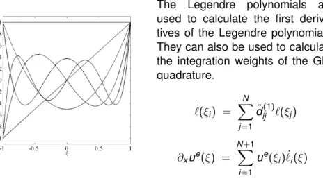
Illustration of Legendre Polynomials

The Legendre polynomials are used to calculate the first derivatives of the Legendre polynomials.

They can also be used to calculate the integration weights of the GLL quadrature.

`(ξ˙ _i) =

N

X

j=1

d˜_ij⁽¹⁾`(ξ_j)

∂xu^e(ξ) =

N+1

Xu^e(ξi) ˙`i(ξ)

(53)

Global Assembly and Solution Global Assembly

Global Assembly and Solution

(54)

Global Assembly for the diagonal of the mass matrix

M_g =





 M_1,1⁽¹⁾ M_2,2⁽¹⁾ M_3,3⁽¹⁾





 +





 M_1,1⁽²⁾ M_2,2⁽²⁾ M_3,3⁽²⁾





 +





 M_1,1⁽³⁾ M_2,2⁽³⁾ M_3,3⁽³⁾







=







M_1,1⁽¹⁾ M_2,2⁽¹⁾ M_3,3⁽¹⁾+M_1,1⁽²⁾

M_2,2⁽²⁾ M_3,3⁽²⁾+M_1,1⁽³⁾

M_2,2⁽³⁾ M_3,3⁽³⁾







(55)

Global Assembly and Solution Global Assembly

Global Assembly for the diagonal of the stiffness matrix

K_g =







K_1,1⁽¹⁾ K_1,2⁽¹⁾ K_1,3⁽¹⁾

K_2,1⁽¹⁾ K_2,2⁽¹⁾ K_2,3⁽¹⁾ 0 K_3,1⁽¹⁾ K_3,2⁽¹⁾ K_3,3⁽¹⁾+K_1,1⁽²⁾ K_1,2⁽²⁾ K_1,3⁽²⁾

K_2,1⁽²⁾ K_2,2⁽²⁾ K_2,3⁽²⁾

K_3,1⁽²⁾ K_3,2⁽²⁾ K_3,3⁽²⁾+K_1,1⁽³⁾ K_1,2⁽³⁾ K_1,3⁽³⁾ 0 K_2,1⁽³⁾ K_2,2⁽³⁾ K_2,3⁽³⁾ K_3,1⁽²⁾ K_3,2⁽²⁾ K_3,3⁽²⁾







(56)

Vector with information on the source

f_g =







f₁⁽¹⁾ f₂⁽¹⁾ f₃⁽¹⁾+f₁⁽²⁾

f₂⁽²⁾ f₃⁽²⁾+f₁⁽³⁾

f₂⁽³⁾ f₃⁽³⁾







(57)

Global Assembly and Solution Global Solution

Extrapolation for time-dependent coefficients u_g

This is our final algorithm as it is implemented using Matlab or Python u_g(t+dt) =dt² h

M_g⁻¹(f_g(t)−K_g u_g(t))i +2u_g(t) −u_g(t−dt)

Looks fairly simple, no?

(58)

Matlab Code: Matrices

% Elemental Mass Matrix for i = 1 : N + 1,

Me(i) = rho(i) * w(i) * J;

end (...)

% Elemental Stiffness Matrix for i = 1 : N + 1,

for j = 1 : N + 1, sum = 0;

for k = 1 : N + 1,

sum = sum + mu(k) * w(k) * Jiˆ2 * J * l1d(i,k) * l1d(j,k);

end

Ke(i,j) = sum;

end

(59)

Matlab Code: Time extrapolation

for it = 1 : nt, (...)

% Extrapolation

unew = dtˆ2 * (Minv * (f - K * u)) + 2 * u - uold;

uold = u;

u = unew;

(...) end

(60)

Spectral elements: work flow

(61)

Point source injection

Top:A point-source polynomial representation (solid line) of a δ-function (red bar).

Bottom:A finite-source polynomial representation (solid line) as a superposition of point sources injected at some collocation points.

For comparison with analytical solutions it is important to note that the spatial source function actually simulated is the polynomial representation of the (sum over)

(62)

sem1d: simulation examples

(63)

Summary

The spectral element method combines the flexibility of

finite-element methods concerning computational meshes with the spectral convergence of Lagrange basis functions used inside the elements.

The enormous success of the spectral element method is based upon the diagonal structure of the mass matrix that needs to be inverted to extrapolate the system in time. Due to this diagonality no matrix inversion techniques need to be employed allowing straight forward parallelisation of the algorithm. The diagonal mass matrix is possible through the coincidence of the collocation

(64)

Summary

The errors of the spectral-element scheme accumulate from the (usually low-order finite-difference) time extrapolation scheme and the numerical integration using Gauss-Lobatto-Legendre

quadrature.

The spectral-element method is particularly useful for simulation problems where the free-surface plays an important role, and/or in which surface waves need to be accurately modelled. Technically the reason is that the free-surface boundary is implicitly solved.

A well engineered community code (SPECFEM3D,

www.geodynamics.org) is available for Cartesian and spherical geometries including global Earth (or planetary scale)