Study of the Neutron-Deficient Nuclei

Software Development for the Analysis of Exotic Beam Experiments and

Study of the Neutron-Deficient Nuclei

98 Cd and ⁹⁸ Ag

Inaugural-Dissertation zur

Erlangung des Doktorgrades

der Mathematisch-Naturwissenschaftlichen Fakult¨ at der Universit¨ at zu K¨ oln

vorgelegt von

Norbert Braun

aus Berlin

K¨ oln 2013

Berichterstatter: Prof. Dr. J. Jolie

Prof. Dr. P. Reiter

Tag der m¨ undlichen Pr¨ ufung: 14.12.2012

All science is either physics or stamp collecting.

— Ernest Rutherford

Abstract

In this thesis, results of an experiment to study exotic nuclei in the

Sn region are presented.

Sn is the heaviest doubly-magic, self-conjugate nucleus. The nucleus and its neighbourhood are an important testing ground for the nuclear shell model, giving input on topics such as the single particle structure or the πν residual interaction. In addition, as the rapid proton capture (rp) process involves nuclei in the region, it is of interest for nuclear astrophysics.

Recently, modern exotic beam facilities have made it possible to study nuclei very far from stability, such as the region around

Sn. Thus, the questions from above can finally be addressed experimentally, and the evolution of nuclear structure can be tracked over a much larger region than previously possible.

The experimental work for this thesis was performed at the FRS ( Fr agment S eparator) instrument at GSI Helmholtzzentrum f¨ ur Schwerionenforschung in Darmstadt, Germany.

Exotic nuclei were produced by fragmentation of an 850 MeV/u

Xe beam on a

Be target. After being separated in the fragment separator they were brought to rest in an active stopper. The Rising high-purity germanium array with 15 Euroball cluster detectors was used to record γ rays and γγ coincidences emitted by isomeric states in the fragmentation products and daughter nuclei from their subsequent β decay. For the daughter nuclei, the active stopper allowed identification via implantation-decay correlation.

I present results for

Cd and

Ag. In

Cd, a previously unknown excited state with an energy slightly below the known (12

) state was discovered, and assigned a tentative spin/parity of (10

). Previous theoretical calculations had predicted this state to lie above the (12

) state. Tentative explanations hint at either a reversal of the neutron νd

/

and the νg

/

single particle orbitals, or an increased proton strength.

In

Ag, evidence for a reversed ordering of the transitions from the two lowest-lying excited states was found. This would change energy and tentative spin assignment for the first (lowest-lying) excited state. In addition, the lifetime of the first excited state was determined. In both cases, reproducing the new results by theoretical calculations yields new insights into nuclear structure in this region.

4

Zusammenfassung

In dieser Arbeit werden Ergebnisse eines Experiments aus der Region um

Sn vorge- stellt.

Sn ist der schwerste, doppelt-magische Kern mit gleicher Protonen- und Neu- tronenzahl. Der Kern und die umliegende Massenregion sind ein wichtiges Testgebiet f¨ ur Theorierechnungen im Rahmen des Schalenmodells, z. B. f¨ ur die Einteilchenstruktur oder die πν Restwechselwirkung. Ferner involviert der rapid proton (rp) Prozess Kerne in dieser Region, weswegen sie auch f¨ ur die nukleare Astrophysik von Interesse sind.

In j¨ ungerer Vergangenheit haben moderne Forschungseinrichtungen zum Studium exo- tischer Strahlen es m¨ oglich gemacht, auch Kerne weit abseits des Tals der Stabilit¨ at zu untersuchen, beispielsweise die Region um

Sn. Dadurch k¨ onnen die oben aufgeworfe- nen Fragen experimentell behandelt werden und die Evolution der Kernstruktur kann uber eine viel gr¨ ¨ oßere Region verfolgt werden, als es bisher m¨ oglich war.

Das Experiment wurde am FRS ( Fr agment S eparator) Aufbau am GSI Helmholtz- zentrum f¨ ur Schwerionenforschung in Darmstadt durchgef¨ uhrt. Die exotischen Kerne wurden durch Fragmentierung eines 850 MeV/u

Xe-Strahls an einem

Be-Target er- zeugt. Nach der Trennung im Fragmentseparator wurden sie in einem aktiven Stopper gestoppt. Mit Hilfe des Rising -Germaniumspektrometers wurden γ-Strahlung und γγ- Koinzidenzen aufgezeichnet, die von isomeren Zust¨ anden in den Fragmentierungsproduk- ten und deren Tochterkernen ausgesandt wurden. Im Falle der Tochterkerne wurde eine Identifizierung durch Implantierungs-Zerfalls-Korrelation mittels des aktiven Stoppers erm¨ oglicht.

Ich stelle Ergebnisse f¨ ur die Kerne

Cd und

Ag vor. In

Cd wurde ein bisher un- bekannter Zustand mit einer Energie knapp unterhalb des bekannten (12

)-Zustands entdeckt. Diesem Zustand wird eine vorl¨ aufiger Spin/Parit¨ at von (10

) zugewiesen.

Theorierechnungen, die vor dem Experiment durchgef¨ uhrt wurden, haben den (10

)- Zustand knapp oberhalb des (12

)-Zustands vorhergesagt. Die experimentellen Ergeb- nisse k¨ onnen durch eine Vertauschung der Neutronen- νd

/

und νg

/

Einteilchen- Orbitale oder durch eine erh¨ ohte St¨ arke der Protonenwechselwirkung erkl¨ arbar sein.

In

Ag wurden Hinweise auf eine vertauschte Reihenfolge der ¨ Uberg¨ ange von den zwei niedrigstliegenden angeregten Zust¨ anden gefunden. Dadurch w¨ urden sich Energie und vermutlicher Spin/Parit¨ at des ersten (niedrigstliegenden) angeregten Zustands ¨ andern.

Außerdem wurde die Lebensdauer des ersten angeregten Zustands bestimmt. In beiden

F¨ allen liefert die Reproduktion der experimentellen Ergebnisse in Theorierechnungen

neue Einsichten in die Kernstruktur dieser Gegend.

Contents

1 Introduction 9

2 Experimental setup 11

2.1 Introduction . . . . 11

2.2 GSI accelerator complex . . . . 12

2.3 FRS fragment separator . . . . 14

2.4 FRS detectors . . . . 15

2.4.1 Scintillators . . . . 16

2.4.2 Time projection chambers (TPCs) . . . . 18

2.4.3 Multiwire proportional counters (MWs) . . . . 18

2.4.4 Multi-sampling ionization chambers (MUSICs) . . . . 18

2.5 Active stopper . . . . 19

2.6 RISING germanium array . . . . 20

2.6.1 γ ray detection with high-purity germanium (HPGe) detectors . . 20

2.6.2 Analysis of HPGe data . . . . 23

2.6.3 RISING . . . . 24

2.7 Data acquistion and trigger system . . . . 27

3 Data analysis 29 3.1 Software: R2D2 . . . . 29

3.1.1 Introduction . . . . 29

3.1.2 Organisation . . . . 29

3.1.3 Unpacker . . . . 31

3.1.4 Calibration . . . . 31

3.1.5 Particle identification . . . . 33

3.1.6 Germanium add-back . . . . 33

3.1.7 Implantation/decay correlation . . . . 34

3.2 Software: HDTV . . . . 37

3.3 Calibration of the RISING array . . . . 39

3.3.1 Calibration sources . . . . 39

3.3.2 Automatic calibration . . . . 39

3.3.3 Technical challenges: the power supply problem . . . . 41

3.4 Calibration of the active stopper . . . . 44

3.4.1 Direct calibration . . . . 44

Contents

3.4.2 Compton scattering calibration . . . . 47

3.5 Transition probabilities . . . . 49

3.6 Halflife determination . . . . 51

4 Experimental results 55 4.1 Particle identification . . . . 55

4.2

Cd . . . . 55

4.2.1 γ transitions . . . . 55

4.2.2 Transition at 4158 keV . . . . 57

4.2.3 Intensity balance . . . . 61

4.3

Ag . . . . 64

4.3.1 γ transitions . . . . 64

4.3.2 Lifetime of the 60.6 keV and 107 keV transitions . . . . 65

4.3.3 Implantation of

Ag . . . . 68

5 Discussion of results 71 5.1 Theoretical description of atomic nuclei . . . . 71

5.2 The nuclear shell model . . . . 72

5.2.1 Shell structure of atomic nuclei . . . . 73

5.2.2 Surface delta interaction . . . . 74

5.3 Shell model calculations for

Cd . . . . 78

5.4 Shell model calculations for

Ag . . . . 81

6 Conclusion 85

8

1 Introduction

In recent years, the study of highly exotic nuclei has become a major focus of nuclear physics. By “highly exotic” we mean nuclei that are so far off the valley of stability that they cannot be produced in low-energy nuclear reactions with stable nuclei. There are two major techniques to produce them: fragment separation, as used in the experiment described in this thesis, and on-line isotope mass separation.

Studies on exotic nuclei are being carried out in a number of facilities around the world, including CERN in Switzerland/France, ILL in France, RIKEN in Japan and the NSCL in the United States. The experiment described in this thesis took place at the GSI Helmholtzzentrum f¨ ur Schwerionenforschung in Darmstadt, Germany, using the FRS ( Fr agment S eparator) instrument. Furthermore, upgraded facilities will become available in the future. An example is the SuperFRS instrument under construction at GSI as a part of FAIR.

One question that drives the study of these nuclei is the evolution of the nuclear shell structure. In the nuclear shell model, there are “magic” numbers of protons and neutrons, roughly analogous to the noble gases in the electronic theory of the atom. The magic numbers manifest themselves as gaps in the single particle energies.

In this thesis, an experiment to study nuclei close to

Sn is described.

Sn is the heaviest nucleus that is both doubly-magic (i.e. has a magic number of protons and a magic number of neutrons) and self-conjugate (i.e. it has the same number of protons and neutrons). To understand nuclear structure in the

Sn region, it is of interest to investigate the neighbouring nuclei, as the nuclear shell model describes them as a

Sn core with additional nucleons or nucleon holes.

An additional motivation to study these highly exotic nuclei comes from the fact that they are involved in the rapid proton capture scenario of nucleosynthesis. Given that present-day theories of nuclear structure are still largely phenomenological in nature, ad- hoc predictions of nuclear properties far from experimentally explored areas are virtually impossible. Therefore, to advance our understanding of nucleosynthesis, experimental access to the regions of the nuclear chart involved in these scenarios is necessary.

100

Sn and the neighbouring nuclei have been subject of a large research effort in the past (see, for example, [1], and many others).

In this experiment, several exotic nuclei in the region around

Sn were studied.

Given the size of this effort, the experiment was done in a large collaboration. For this thesis work, I analyzed data pertaining to the nuclei

Cd and

Ag.

The rest of this text is organized as follows:

1 Introduction

• Chapter 2 discusses the experimental setup (accelerators and detectors) in more detail. The detectors used can be divided into three major groups: FRS detectors (particle identification), HPGe detectors (γ-ray spectroscopy) and silicon detectors (active stopper, decay product spectroscopy).

• Chapter 3 reviews the various steps needed to reduce the raw data to experimen- tal results. The chapter presents the R2D2 analysis software in more detail and discusses the steps needed to calibrate the HPGe and silicon detectors.

• Chapter 4 presents the experimental results on

Cd and

Ag.

• Chapter 5 compares the experimental results to theory. The nuclear shell model is introduced and two possible explanations for the results on

Cd are discussed.

In addition, first shell model results on

Ag are shown.

10

2 Experimental setup

2.1 Introduction

As mentioned in the general introduction, there are two major techniques for producing exotic nuclei. The first one is on-line isotope mass separation, of which the ISOLDE facility at CERN is a major example. At ISOLDE, a beam of protons is accelerated to an energy of the order of 1 GeV and impacted on a uranium target. Inside the target, spallation, fission, and fragmentation reactions produce a wide range of exotic nuclei, which end up at rest. They are removed from the target by thermal diffusion at high temperatures (above 1000

C) and fed into a mass separator, where again the isotope of interest is selected for further study. It is possible to re-accelerate the exotic nuclei to study them in nuclear reactions, using the post-accelerator REX. It is not essential to use a proton beam; other ISOL facilities have used heavy ions. As the ISOL technique did not play any role for this thesis, it will not be described in further detail.

For this work, the fragment separation technique was used. In this method, a beam of stable, heavy nuclei is accelerated to high energies (hundreds of MeV per nucleon for our experiment) and impacted on a fragmentation target consisting of light nuclei. In the fragmentation target, the heavy nuclei split up into a cocktail of fragmentation products with a wide range of possible proton and neutron numbers. These fragmentation prod- ucts are still travelling at a large fraction of their original speed. They are then sorted by their deflection in magnetic fields and studied.

The experiment took place at the FRS fragment separator at GSI (Gesellschaft f¨ ur Schwerionenforschung ). A primary beam of

Xe was accelerated to an energy of 850 MeV per nucleon and then fragmented on a

Be target with a thickness of 4 g/cm

. The fragments were sorted using the FRS (fragment separator), then slowed down and finally stopped in an active stopper (active means that the stopper itself is a detector, see below).

The separation of the fragments happens on two levels. The first level is the FRS.

However, the FRS is not setup to pass only a single isotope. Instead, various detectors inside the FRS enable us to identity every particle individually. By sorting the events electronically, we can thus run studies on various isotopes at once.

The fragmentation reaction produces the fragment nuclei in a highly excited state.

Unfortunately, the typical lifetime of these excited states is small compared to the travel

time through the FRS (roughly 300 ns). Therefore, nuclei only have a chance to arrive

at the stopper in an excited state if they have long-lived (isomeric) states with a lifetime

2 Experimental setup

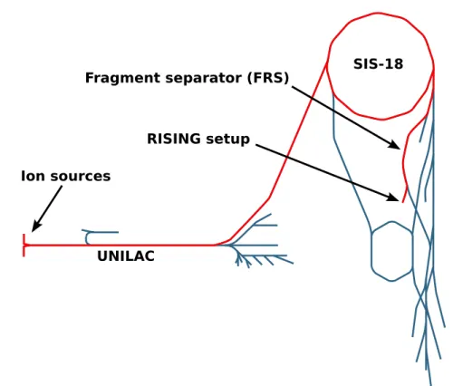
Ion sources

UNILAC

SIS-18 Fragment separator (FRS)

RISING setup

Figure 2.1: Schematic view of the GSI accelerator complex. The beam path relevant for our experiment is highlighted in red.

larger than or comparable to the travel time through the FRS. To study the γ decay of these isomeric states, the active stopper is surrounded by a large array of HPGe (high-purity germanium) detectors, the RISING array.

Eventually, the nuclei inside the stopper will decay. The stopper is formed by a silicon detector, so the decay products can be measured. Usually, the particle decay will populate excited states in the daughter nucleus, the γ decay of which can also be measured with the Ge array.

2.2 GSI accelerator complex

The GSI is a large nuclear/particle physics research facility located near Darmstadt, Germany. Nuclear physics research topics include exotic nuclei, super-heavy nuclei and high-precision mass measurements.

GSI started with a linear accelerator called UNILAC. Later, the heavy ion synchrotron SIS-18 was added. Accelerator beamtime is shared between the experiments. The frag- ment separator FRS uses the beam from the SIS-18.

A schematic overview of the beam path from its source to the experiment is shown in

12

2.2 GSI accelerator complex

Figure 2.2: The UNILAC linear accelerator at GSI (from [2]).

Figure 2.3: The SIS18 synchrotron at GSI (from [4]).

fig. 2.1. At the beginning of the acceleration process, an ion source produces positively charged ions from neutral xenon gas. The entire source setup is on high potential with respect to ground, which accelerates the exiting ions to the injection energy of 2.2 keV/u.

The ions then enter the UNILAC linear accelerator (fig. 2.2 and [2]), which accelerates the ions to an energy of 11.4 MeV/u (standard value, from [3]). Inside the UNILAC, a gas stripper removes further electrons from the already accelerated ions, thus increasing their charge and enabling higher energy gains in the following UNILAC section. After the UNILAC, the ions pass a second (foil) stripper. At this point, their energy is high enough for the stripper to remove all (or almost all) remaining electrons.

The major share of the acceleration, from 11.4 MeV/u to 850 MeV/u, happens in the

SIS-18 (from German: Schwerionensynchrotron ; fig. 2.3 and [4]). The SIS-18 is a 216 m

2 Experimental setup

circumference synchrotron. The particles are injected, then accelerated, and finally fed to the production target. The ejection of a bunch of particles onto the production target is called a spill. A spill has a typical duration of the order of one second, with spills being of the order of seconds apart. A fast spill repetition rate requires the magnetic field strength in the SIS to vary quickly, which needs large power supplies (tens of MWs) to remove and supply the energy stored in the magnets.

Between the injection of particles into the SIS, the UNILAC would normally be idle.

There are, however, a number of experiments for which the UNILAC energy is sufficient.

By quickly switching ion sources at the entrance and beam lines at the exit, these experiments can share the UNILAC with the SIS. Therefore, a UNILAC-only and a SIS experiment will typically run in parallel.

2.3 FRS fragment separator

The high-energy xenon ions can now be fragmented to produce the exotic nuclei of inter- est. It is clear that the fragmentation is a stochastic process, producing a large number of possible fragments. In order to study a specific nucleus of interest, it is required to identify them. While electronic event-by-event particle identification is employed in our experiment (see detailed description below), the production rates for fragments near the valley of stability are so much greater than those for highly exotic fragments that no reasonable system could handle the total event rate required. Therefore, a two-step pro- cess is employed where the fragment stream is first filtered by a system of magnets and slits and event-by-event particle identification is only used on the part of the fragments that remain.

Fig. 2.4 shows a simplified overview of the FRS. The primary xenon beam enters from the left and hits the fragmentation target. The fragments then enter the first sorting stage, consisting of two dipole magnets.

To understand the sorting process, consider the motion of a relativistic particle in a constant magnetic field with the field vector perpendicular to the particle velocity [5].

The resulting motion is circular, with the radius ρ given by γm v

ρ = qvB (2.1)

where m and q are the particle mass and charge, v is the magnitude of its velocity, c is the speed of light, B is the magnitude of the magnetic field and

β = v

c and γ = 1

√ 1 − β

(2.2)

as usual. Let us assume that all fragments are fully stripped nuclei. Their charge is then given by q = eZ , where e is the elementary charge and Z is the number of protons in the

14

2.4 FRS detectors

F ragmen tation target Magnets

S2 area

Degrader T oF scin tillator (s tar t) Magnets MW detector (p osition) T oF scin tillator (s top )

S4 area

Activ e stopp er

Rising arra y V eto scin tillator

Figure 2.4: FRS overview (simplified).

nucleus. For the mass, we get m = m

A, where m

= m

≈ m

is the proton/neutron mass and A is the mass number of the nucleus.

Equation 2.1 can now be rewritten to read Bρ = m

c

e

√ β 1 − β

A

Z = const · A

Z (2.3)

which implies that the deflection in a magnetic field can be used to sort fragments with equal velocity by their A/Z ratio. This alone is not sufficient, so a sorting step by Z is required next.

By the Bloch equation, the energy loss ∆E of charged particles passing through matter is

∆E ∝ Z

f (β) (2.4)

A piece of matter in the beam (degrader) after the A/Z sorting step will therefore slow down the fragments depending on their Z . In the next pair of magnets, A/Z is now constant, but v (and therefore β) is now dependent on Z, so that the radius effectively depends on Z. This allows for the desired sorting based on Z.

Details on the FRS may be found in [6].

2.4 FRS detectors

In order to further enable the event-by-event electronic particle identification, the FRS

is equipped with various detectors. Fig. 2.4 gives a coarse overview. Fig. 2.5 shows the

2 Experimental setup

bruenle FRAME 1 APRIL 16, 2008 17.26.32

ª

£ £

££

ª £

£

£ ££ £Beam

MW 2.1 £££££££ £

££

604 1013

1228 1554,5

1782,5 1907,5

2012,5 2203,5

Y−Slits X−Slits SCI Ladder MW 2.2 CG Degr. Disc var.Degrader Degrader Plates 2397,5

Aperture ££

15.04.08

£

££

£££ £ £

£

£ £ £

2798 3965

4115

TPC 2.1 TPC 2.2 Nb − Foil 260um thick

Ti−Window 200um thick 250mm diameter Fe−Window

100um thick 120x200mm

Figure 2.5: Setup of the S2 area of the FRS [7].

exact setup of detectors (as used in this experiment) in the area between the magnet pairs (S2 area, refer to fig. 2.4) and fig. 2.6 shows the detectors at the exit of the FRS (S4 area).

The electronic particle identification is explained in detail in section 3.1.5. The mea- surements needed include precise timings for time-of-flight (ToF), giving access to the particle velocity, position measurements, giving access to the path of the particle through the magnet and thus the curvature radius, and energy loss measurements, giving access to the particle charge via the Bethe-Bloch equation. The various types of detectors used will now be described in detail.

2.4.1 Scintillators

Scintillator detectors are based on materials that emit light when charged particles pass through them and deposit energy. The light is then detected, typically by using

16

2.4 FRS detectors

bruenle FRAME 1 JULY 10, 2008 16.32.40

ª ^{9 t} £ ££ £ £

££

£

££ £ £

£ £££

£

FRS, S4, S352, 124Xe3+, Blazhev/Gorska Juli 08 03.07.08

££

£

£ £

£ £££

£ £

£

£ MW 4.1 Mucic 1 Mucic 2 SC| 3.15mmSlitsMW 4.2 Degrader

£££ £

£ £ £

£ £ ££

1280

* *

1140 940

* *

1845

* *

2385

* *

2600

* *

2720

* * £

3040

* *

3250

* *

TPC 5 TPC 6 £

3470

* * SCI

Figure 2.6: Setup of the S4 area of the FRS [7].

2 Experimental setup

photomultiplier tubes.

The amount of light generated is proportional to the energy deposited, so the detectors can be used for energy loss measurements. The energy resolution is limited by the number of photons reaching the photomultiplier tube and the resulting counting noise.

Scintillator detectors are fast (FWHM timings of the order of tens of ps). By using photomultiplier tubes on either side of the scintillator, they can also be made position sensitive (FWHM of the order of a few mm).

2.4.2 Time projection chambers (TPCs)

Time projection chambers are gas-filled chambers where charged particles leave tracks of ionized gas. A high electric field separates the charges and transports them to the end plates, where they are detected. The position along the electric field is determined from the time of flight, whereas the position tangential to the electric field can be determined via segmented detectors at the end plates.

2.4.3 Multiwire proportional counters (MWs)

The multiwire proportional counter is a position sensitive detector. Particles passing through the gas-filled detector create ions which then drift in an electric field and are amplified via an avalanche effect. Finally, the avalanche hits the anode. Close to the anode, two sets of perpendicular cathode wires are located. The avalanche hitting the anode induces a current pulse on the nearest cathode wires. The difference in charge collected on either end of the cathode wire gives the position of the avalanche along that wire. As there are two perpendicular sets of cathode wires, an (x,y) position can be reconstructed.

2.4.4 Multi-sampling ionization chambers (MUSICs)

The Multi-Sampling ionization chamber is used to measure the charge of the particles.

It consists of a gas-filled chamber where the beam particles cause ionization as they pass through. There are eight anodes in the chamber, each collecting charge from a defined region. Thus, the MUSIC produces eight signals. In the analysis, they are combined by rejecting two outliers and averaging the six remaining measurements.

In order to keep the load on the extremely thin entry and exit windows of the MUSIC as low as possible, the gas inside the detector is at ambient pressure. For longer experi- ments, this implies that the gas pressure (and thus the gas particle density) varies over time.

18

2.5 Active stopper

(15,15)

(0,0) y

x

(15,15)

(0,0) y

x (15,15)

(0,0) y

x

Column 0 Column 1 Column 2

Layer 0 Layer 1

Layer 2

Beam

Up

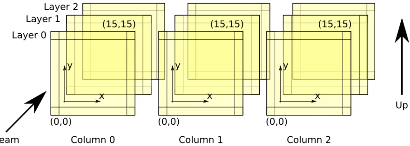
Figure 2.7: Layout of the active stopper detector. (For compatibility with the anal- ysis software, a numbering convention starting at 0 is used, like in the C programming language.)

2.5 Active stopper

The experiment described in this thesis uses the setup in stopped-beam mode, meaning that the nuclei of interest are studied after they have come to rest inside a suitable stopper. After implantation in the stopper, the unstable nuclei eventually decay (in the case of neutron-deficient nuclei, usually by β

decay). To be able to study the particle decay products as well, an active stopper is used.

The β-lifetime of our exotic nuclei is much larger than the time between the two nuclei hitting the stopper (seconds vs. milliseconds). This means that, if a β decay takes place, the parent nucleus is unknown. The problem is solved by using a segmented silicon detector as the stopper (active stopper). This allows for implantation-decay correlation.

Remember that, at implantation time, the nucleus being implanted in known (from the FRS particle identification). If we remember the implantation position, the parent nucleus in a subsequent decay at the same position is known. For the technique to work, the implantation rate in a given silicon pixel must be less than the β lifetime.

Our active stopper consists of double-sided silicon strip detectors (DSSSDs). In these detectors, both sides are segmented in strips, with the strips on one side being orthogonal to those on the other side. If there is a single event in a given time window, this arrangment allows the determination of an x and a y coordinate, effectively giving a pixelated detector (but with far less channels to read out). The drawback versus an actual pixelated detector is, of course, that an ambiguity results for two or more events in the time window and the positions can no longer be uniquely determined. Our detectors have 16 strips per side, yielding effectively 256 pixels per detector.

The geometric arrangement of the detectors in shown in fig. 2.7. There are a total of

9 DSSSDs, arranged in 3 layers of 3 detectors each. The size of each detector is 5x5cm,

with a thickness of 1mm.

2 Experimental setup

2.6 RISING germanium array

2.6.1 γ ray detection with high-purity germanium (HPGe) detectors

In this section, the physics of γ detection using HPGe detectors will be briefly described.

These detectors are essentially semiconductor diodes operated in reverse direction, with the voltage chosen high enough that the entire detector volume is depleted. Current can only flow if electron-hole pairs are generated in the depleted region. The energy from γ quanta being absorbed in the detector will ideally go completely to the production of electron-hole pairs. As the energy required to generate a single electron-hole pair is constant, the absorption of a γ quantum in the detector will generate a current pulse whose integral (i.e. total charge) is proportional to the energy of the γ quantum.

Of course, the idealized picture is not entirely correct. The energy from the γ quantum can go either to the creation of electron-hole pairs or to lattice vibrations (phonons).

This is a statistical effect, so the number of electron-hole pairs created from a γ quantum of a given energy will vary, creating noise. In addition, inevitable impurities in the crystal create energy levels inside the band gap. These can lead to electron-hole pairs recombining or not arriving at the detector electrodes inside the collection time window (trapping). A third noise source is the inevitable noise created in the electronic circuits required to register the current pulse.

There are three mechanisms by which γ radiation interacts with matter: photo effect, Compton effect and pair production. In the photo effect, the γ quantum is completely absorbed and its entire energy is transmitted to an electron (which then creates electron- hole pairs). In the Compton effect, the γ quantum is scattered by an electron and only transmits part of its energy. Pair production refers to the creation of an electron-positron pair from the γ quantum. For this effect to be possible, the γ energy has to be at least the rest mass of the electron and the positron (2 · m

= 1022 keV). (Note that pair production from a single γ quantum cannot happen in a vacuum due to the conservation of momentum. In the detector, however, an atom from the detector material can take the momentum.)

In practice, two or all three of the effects mentioned can happen during the absorption of a single γ quantum. The γ might, for example, first produce an electron-positron pair. The kinetic energy of the electron and the positron creates electron-hole pairs.

The positron will eventually annihilate with an electron from the detector material, producing (typically) two new γ quanta with an energy of 511 keV each. These may then undergo Compton scattering until they are finally fully absorbed by the photo effect. The timescale on which such a sequence of events happens is so short that the detector electronics cannot resolve it (it may, however, be able to resolve the different positions where the events took place; see below).

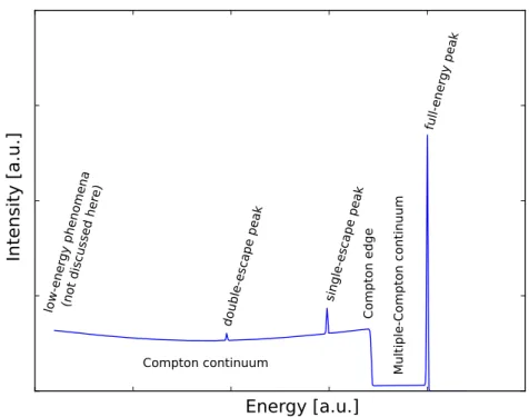
Fig. 2.8 shows the schematic energy spectrum produced by monoenergetic γ radia- tion in the detector. (We assume that the energy of the radiation is above the pair production threshold.) The rightmost peak is the full-energy peak (sometimes called

20

2.6 RISING germanium array

Intensity [a.u.]

Energy [a.u.]

low-ener gy phen

omena

(not disc ussed h

ere)

single-esca pe peak

double-escape peak

full-ener gy peak

Compton continuum Multiple-Compton continuum

Compton edge

Figure 2.8: Schematic energy spectrum for the interaction of monoenergetic γ radiation with a germanium detector. γ energy assumed to be above the pair produc- tion threshold. (See text for explanation.)

the photopeak), corresponding to events where the full energy of the γ quantum was absorbed in the detector. 511 keV below it is the single-escape peak. It corresponds to events where pair production took place and one of the annihilation γ quanta escaped the detector without further interaction, while the rest of the original γ energy was com- pletely absorbed. Likewise, the double-escape peak 1022 keV below the full-energy peak corresponds to events where both annihilation quanta escaped the detector. The con- tinuum corresponds to γ quanta that left the detector again after undergoing Compton scattering and depositing part of their energy.

Consider the scattering of a γ quantum on an electron initially at rest. Conservation of four-momentum implies a connection between the initial γ energy E

, the final γ energy E

and the scattering angle θ:

1 E

− 1

E

= 1

m

c

(1 − cos θ) (2.5)

The energy difference E

− E

goes into kinetic energy of the electron and finally into creation of electron-hole pairs, which are then detected. Rearranging the equation gives an expression for this energy difference:

E

− E

= E





1 − 1 1 +

ec²

(1 − cos θ)





(2.6)

2 Experimental setup

From the equation, it is apparent that the γ quantum cannot transmit its entire energy in a single Compton scattering event. This gives rise to the Compton edge at an energy

E

= E





1 − 1 1 + 2

ec²





(2.7)

Obviously, this analysis is valid only for a single Compton scattering event. As there is a small probability that the γ quantum undergoes multiple Compton scatterings before leaving the detector again, the gap between the Compton edge and the full-energy peak is filled by a smaller multiple-Compton continuum.

The probability for Compton scattering is dependant on the scattering angle θ, and thus on the energy transmitted. The Compton continuum is therefore not flat, but slightly curved. In lowest order of quantum electrodynamics, the angle-dependent Comp- ton scattering probability is given by the Klein-Nishina formula [8]. The derivation is rather involved, so it will not be discussed further.

Software packages exist which can simulate the HPGe detector response to γ rays with given energies using Monte-Carlo techniques. Geant is one example ([9], [10], [11]).

In actual measurements, where γ rays with several discrete energies are to be detected, the complex detector response of germanium detectors causes some problems. The Compton background is the most severe. Given finite statistics, the Compton contiuum will be subject to Poisson (counting) noise. The noise in the Compton continuum from a high-intensity γ ray may completely swamp the full-energy peak of a lower-energy, lower-intensity γ ray. As such, it is highly desirable to reduce the Compton continuum.

The traditional way of doing this is to surround the germanium detector with anti- Compton shields. These shields are scintillators made from bismuth germanate (BGO).

Due to the high Z of the scintillators, a γ ray entering them is highly likely to be detected. Unfortunately, the energy resolution of the scintillators is rather poor. They can therefore only be used as a veto, meaning that events where the scintillator saw something are thrown away. With anti-Compton shields, the Compton background can be significantly reduced. It cannot be completely eliminated, however, because the side of the Ge detector looking at the γ source must stay open, and there is a certain probability of Compton scattering under an angle of almost 180

.

A highly sophisticated modern alternative is used in γ arrays such as AGATA [12].

These arrays surround the γ source with essentially a hollow sphere of detector material.

This makes it highly likely that a Compton scattered γ is eventually absorbed in another detector, and its total energy can be reconstructed by summing the measurements in the different detectors. A complication arises because typically, multiple γ rays are emitted from the source simultaneously. To disentangle the events from the various original γ rays, highly segmented, position sensitive detectors and maximum-likelihood methods are used.

22

2.6 RISING germanium array

2.6.2 Analysis of HPGe data

In an actual experiment, there is typically no interest in the details of the HPGe detector response, but in the (discrete) energies and the intensities of the original γ rays. This is normally done by peak fitting. Usually, only the full-energy peak is considered. The shape of the full-energy peak is nearly Gaussian under ideal circumstances. A common source of deviations from that shape is neutron damage, where the crystal structure of the detector material has been damaged by neutrons. This results in a low-energy tail in the peak shape. Precise modelling of the tail is difficult, so empirical descriptions are used, several of which have been proposed over the years.

As mentioned already, the full-energy peak sits atop the Compton continuum from higher-energy γ rays. Again, precise modelling of the Compton continuum is difficult.

It is therefore approximated by an empirical formula, e.g. a polynomial, in the vicinity of the peak of interest. In practice, one manually chooses two peak-free regions left and right of the peak of interest and fits the background description to these regions. In the next step, the chosen peak description is fitted to the actual peak, with the background substracted. If two peaks partly overlap, they can be separated by fitting the sum of two peak descriptions.

The method described here has a number of drawbacks. In peaks with tails and high statistics, it is normally found that even the best parameters for the empirical shape deviate from the actual data in a statistically significant manner. The accuracy of peak position and integral obtained from the empirical description is therefore questionable.

Also, the position and integral error calculated by the fitter is then mostly meaningless.

In practice, the errors are usually estimated rather than obtained as results of the fitting process.

The second drawback of the method is that the identification of the peaks, and the selection of the peak-free regions used for background fitting, are a completely manual process. In cases where the number of spectra to be analyzed is large, or there are many peaks in each spectrum, this quickly become a laborious, dull, and error-prone task. Apart from that, the results obtained now depend on (partly) subjective choices made by the person analyzing the data, which makes a rigorous error analysis even more difficult.

In the experiment described in this thesis, the number of peaks of interest was for- tunately small. An exception is the energy calibration of the detectors, which requires fitting some ten peaks in about 100 spectra. In that case, however, one has additional information about the expected peaks present in the spectrum and their positions (be- cause the energy calibration can be assumed to be nearly linear). This allows to tolerate a certain number of false positives/false negatives from a less-than-perfect heuristic for peak finding. Still, some detectors with significantly worse peak widths required man- ual intervention. The automatic Ge energy calibration developed during this work is described in further detail in section 3.3.

After the peak positions and integrals have been determined, we need to convert them

2 Experimental setup

to energies and (relative) intensities. For converting the peak positions, we need an energy calibration of the detector. As was already mentioned, the charge pulse generated in the detector is roughly proportional to the energy deposited (which is equal to the energy of the γ quantum in case of the full-energy peak). We thus need to determine the constant of proportionality between ADC (analog-to-digital converter) channels and γ energies. This is done by using a γ source with known energies. In practice, the relation between ADC channels and energies turns out to also include an offset and (small) non- linear terms. The relation between ADC channels c and energies E(c) is described by a polynomial,

E (c) =

N

X

i=0

a

c

with the order N typically three or less, and the expectation that the higher-order terms a

c

, . . . be small.

For converting full-energy peak integrals to (relative) intensities, we need an efficiency calibration, i.e. we need to know how likely a γ quantum of a certain energy is to be fully absorbed in the detector. Given the complexity of the interaction between γ radiation and the detector described above, a simple relation for this energy dependance is not expected. In fact, it turns out to be sufficiently complex that an analytical description is normally not attempted. (Note, however, that Monte Carlo simulations, as mentioned above, can describe the relation fairly well.) In practice, the calibration data is fitted with an empirical formula having a large number of parameters (up to seven).

The popular RadWare [13] package uses a function of the type (E

) = exp

(A + B ∗ x + C ∗ x ∗ x)

+ (D + E ∗ y + F ∗ y ∗ y)

(2.8) where x = log(E

/E

) and y = log(E

/E

), and E

= 100 keV and E

= 1 MeV are fixed.

Another empirical formula was first proposed by I. Wiedenh¨ over [14]

(E

) = A exp (−B ln(E

− C + D exp(−EE

))) (2.9) Non-linear fitting has severe problems with local minima and sensitivity to starting parameters. It might therefore be objected that, if an empirical formula is fitted anyway, the non-linear fit is best avoided. A better idea may be to fit a polynomial to the log(energy)/log(efficiency) plot, as discussed in [15]. (Note that fitting a polynomial is a linear fit.)

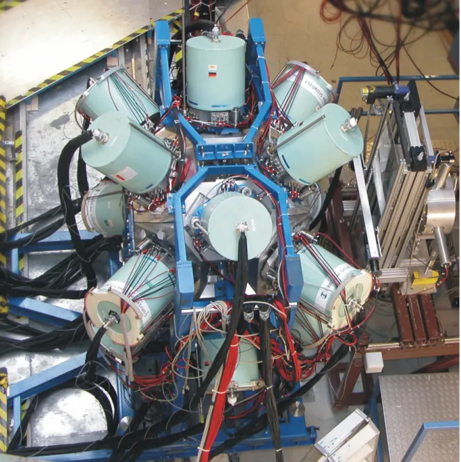
2.6.3 RISING

The Rising (Rare Isotope Spectroscopic INvestigation at GSI) array consisted of 105 non-segmented HPGe detectors (it has since been decommissioned). Seven detectors

24

2.6 RISING germanium array

Figure 2.9: Photograph of the Rising setup (Jerzy Gr¸ebosz, Instytut Fizyki J¸ adrowej,

Krakow).

2 Experimental setup

0 1

2

3

4

5 6

Figure 2.10: Arrangement of detectors in a Euroball cluster.

form a Euroball cluster [16], for a total of 15 clusters in the array. The detectors in a cluster are packed close together in a common cryostat (see fig. 2.10).

As mentioned, the exotic nuclei in the experiment described in this thesis decay in the active stopper, i.e. at rest. The decay γ radiation is thus emitted isotropically.

The detectors are distributed evenly around the stopper (the so-called stopped beam configuration of the array). Fig. 2.9 shows a photograph of the setup. The photopeak efficiency, i.e. the fraction of γ quanta emitted at the stopper which are fully absorbed and detected in a detector of the array is estimated at around 10% at 1.3 MeV. (Note that the efficiency is highly dependent on the energy of the γ quanta.) Because of technical problems, only 99 of the 105 detectors could be used for this experiment.

The clusters can be equipped with anti-Compton shields, this, however, is not done for Rising . The only anti-Compton measure used is add-back, i.e. the addition of simultaneous energy depositions in neighbouring detectors in a cluster. This is described in more detail in section 3.1.6.

The output signal of every germanium detector needs to be processed to accurately determine the amount of charge generated for a given event. Previously, this was done using analog electronics (the shaping or main amplifier). Today, this processing is in- creasingly done digitally. The signal from the detector preamplifier is fed into a sampling ADC (analog-to-digital converter). The shaping is then done in software, using a combi- nation of an FPGA (field-programmable gate array) and a DSP (digital signal processor).

This digital processing is actually essential to achieve the position sensitivity in arrays such as Agata (pulse shape analysis). In non-position sensitive detectors, it is merely convenient and cheaper.

The Rising array uses XIA DGF (digital gamma finder) modules [17] to perform the digital processing. These modules largely imitate the function of the earlier analog electronics. They detect charge pulses in the detector, digitally determine the amount of charge, and store it together with a timestamp. Additionally, they support external gates, which make the storage of an event dependent on certain conditions (whether

26

2.7 Data acquistion and trigger system

quasi-simulataneous events were seen by other detectors, for example). This helps to keep the data rate manageably low.

Details on the Rising array can be found in [18].

2.7 Data acquistion and trigger system

The data acquisition system is based on the notion of events. There are two main types of events: implantation and decay events. An implantation event corresponds to the arrival of a nucleus in the active stopper; in a decay event, a nucleus in the active stopper undergoes particle decay.

After each event, the relevant data from the detectors is read out and stored. It should be noted that an event can contain several sub-events. If, for example, an excited nucleus is implanted in the stopper and decays via a cascade, several γ quanta could be detected.

The timing information for these sub-events is generally relative to the event trigger.

High-resolution relative timing information is only available for sub-events within the same event, but a 1 kHz scaler that is read out at each event provides low-resolution timing across events.

The event-based notion of the data acquisition system extends even to the XIA mod- ules. These modules have a FIFO (first-in first-out) buffer from which the accepted γ events can be read, together with a timestamp, so, in principle, they could be read out asynchronously. For compatibility with the rest of the data acquisition system, however, they are read out once per event. The event trigger is fed to a special channel in one XIA module, so that the internal timestamps can be synchronized to the event timing.

In addition to the XIA modules internal timestamp (40 MHz clock), there are two TDC (time-to-digital converter) based Ge timing systems. The long-range TDCs are based on special chips developed at CERN. Each module (CAEN v767) provides 128 channels with multihit capability and 800 ps LSB resolution (LSB = least significant bit, i.e., for this device, a change in the value by one corresponds to 800 ps). In addition, there are short-range TDC modules with approx. 300 ps LSB resolution. The timing system for the Si strips uses the same modules.

An implantation event takes place when a particle traverses the FRS and is stopped in the active stopper. Such an event is triggered by a scintillator in front of the stopper (Sci41 or Sci42). The main data from such an event are the particle identification infor- mation, possible radiation emitted directly after the implantation, and an implantation position from the active stopper.

A decay event is triggered by the active stopper. The active stopper registers a position

for later correlation and the decay energy. In addition, if the decay ends in an excited

state in the daughter nucleus, the Rising array registers γ energies and times from the

subsequent de-excitation.

3 Data analysis

3.1 Software: R2D2

3.1.1 Introduction

The software package used for the analysis of the data is called R2D2. It is based on the ROOT data analysis framework [19] developed at CERN. R2D2 was initially devel- oped for the analysis of the first RISING stopped beam experiment (Feb. 2006,

Ag beam) and then substantially upgraded and extended for the analysis of the experiment described in this thesis.

For this analysis, R2D2 provided the following services:

• Unpacking of the listmode data

• Application of energy and time calibration (for all detectors where it is needed)

• Germanium cluster add-back

• Reconstruction of implantation positions from silicon data

• Implantation-decay correlation

All of these will be described in more detail below.

3.1.2 Organisation

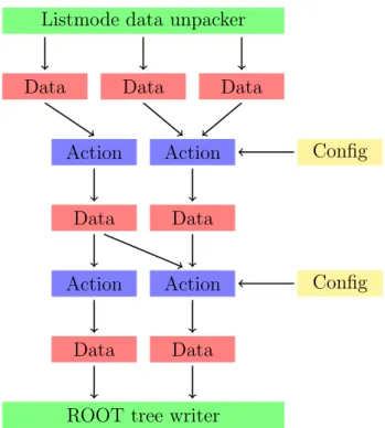
R2D2 is designed to be modular, so that other experiments with potentially different setups or requirements can easily reuse the relevant parts of it. To achieve this modu- larity, the concept of actions operating on the data stream is used. The idea comes from the analysis software used by the ALADIN collaboration at GSI, developed under the leadership of Walter M¨ uller.

The concept is illustrated in fig. 3.1. We assume that the data comes in events, i.e.

groups of detector readings that lie close together in time. The unpacker reads one full

event from the listmode data stream. For efficiency reasons, we use data containers that

are allocated once and get re-filled (i.e. overwritten) at each event. Each action class

takes one or several data containers as input and fills one or several data containers with

its output. Action class input data that does not change for each event (e.g. coefficients

of calibration polynomials) is called configuration and stored in configuration classes.

3 Data analysis

Listmode data unpacker

Data Data Data

Action Action Config

Data Data

Action Action Config

Data Data

ROOT tree writer

Figure 3.1: Illustration of the R2D2 data flow (see text).

Asc (Scalers)

Afrsraw Afrsp Afrsid FRS branch

Ageraw Agecal

Ageab Ge branch

Asiraw Asical Asipos Asipixels Si branch

Figure 3.2: Branches (detector groups) in the R2D2 software.

30

3.1 Software: R2D2

At the end of the action chains, the processed data is stored in a ROOT tree, again on an event by event basis. Note that R2D2 does not handle histogramming of data from different events, except for debugging. There is a separate software, called C3PO, to generate the final histograms.

3.1.3 Unpacker

The first task in R2D2 is to extract the data from the listmode data stream. The data stream essentially consists of raw data as received from the various electronic modules, with very little processing applied to them. The unpacker needs experiment-specific lookup tables to determine which VME bus addresses correspond to which devices, and device-specific code to convert raw register values into ADC/TDC readings. At the end of the unpacking state, the data consists of concrete ADC/TDC readings corresponding to concrete detectors.

There are three main groups of detectors (called branches): the germanium branch (the RISING array), the silicon branch (the active stopper), and the FRS branch. The first two branches are homogeneous, i.e. they consist of a large number of detectors which are all alike. The third branch consists of many different types of detectors. In addition, there are a number of scalers (counters) which are processed (fig. 3.2).

3.1.4 Calibration

In the next step, the raw ADC/TDC readings need to be converted to physical quantities, i.e. deposited energy and time (difference). This is done by applying a calibration function, E(c) or T (c), where E or T are physical energy or time, and c is a raw ADC/TDC channel. The functions are usually linear, E(c) = a

c + a

. They are determined by measuring data with known characteristics. The calibration process is described in more detail in section 3.3 (germanium detectors) and section 3.4 (silicon detectors).

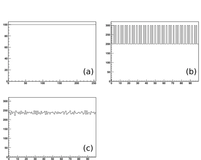
A slight subtlety is illustrated in fig. 3.3. Consider a histogram of the energies of all

events. Every ADC channel will, after the calibration, correspond to a certain energy and

thus fall in a certain energy bin. Typically, the number of ADC channels corresponding

to a certain energy bin will not be constant, but vary from energy bin to energy bin. This

will introduce a variation of the bin contents in the energy histogram, even if the initial

number of events per ADC channel was constant (fig. 3.3 (a) and (b)). The problem is

solved by a technique called dithering. A random number from the range (-0.5, 0.5] is

added to each ADC reading before application of the calibration function. Note that this

does not destroy any information; the original ADC channel can be exactly recovered

by rounding. However, the values are now “spread out” over the width of the channel

and, after calibration, evenly distributed over the possible energy bins. The result, as

shown in fig. 3.3 (c), is that data with a flat distribution over ADC channels now results

in an energy histogram that is also flat (except for Poission noise).

3 Data analysis

0 50 100 150 200 250

0 20 40 60 80 100

0 10 20 30 40 50 60 70 80 90

0 50 100 150 200 250 300

0 10 20 30 40 50 60 70 80 90

0 50 100 150 200 250 300

(a) (b)

(c)

Figure 3.3: Demonstration of dithering: (a) simulated raw ADC spectrum, 256 bins, 100 counts per bin (b) result of “calibrating” the histogram with E = 0.42 · c and re-binning with 100 bins: semi-regular structure appears (c) the same operation with dithering: the structure is reduced in amplitude and no longer regular.

32

3.1 Software: R2D2

3.1.5 Particle identification

The next major step in the data processing is to turn the information from the FRS detectors into a particle identification. As noted before, particle identification is only possible for implantation events; for decay events, implantation-decay correlation, as described below, will have to be used.

In order to fully identify the nuclei, two quantities have to be determined: A/q (mass over charge) and Z (nuclear charge). Determination of A/q works similarly to the magnetic sorting in the FRS, as described in section 2.3, and makes use of the formula

Bρ = m

c e

√ β 1 − β

A

q (3.1)

m

(nucleon mass), c and e are simply constants. The magnetic field B in the magnets can be measured using Hall probes or Nuclear Magnetic Resonance techniques; also, it is expected to be mostly constant during the experiment. This leaves β :=

/

and the curvature ρ to be determined.

The curvature ρ follows from measuring the position of the particle as it passes through the S2 and S4 areas. As the particle identification is essential for the experiment, several independent position measurements are made, using scintillators and time projection chambers (TPCs).

Determining the beam particle velocity β =

/

requires knowledge of the path taken, i.e. the curvature ρ, and the time-of-flight. The latter can be measured with high accu- racy by a pair of scintillators. Again, several measurements are taken for redundancy.

The determination of the nuclear charge Z makes use of multi-sampling ionization chambers (MUSICs). As described in section 2.4.4, the MUSIC detectors measure the ionization of gas by the beam particles. By the Bethe formula, the energy deposited will depend on the beam particle charge q, the beam particle velocity β, and the gas particle density. The gas inside the MUSIC is at ambient pressure and temperature, which are measured during the experiment and used to calculate the gas particle density. β is also known (see above), allowing the charge q of the beam particles to be determined. It should be noted that q is not equal to the nuclear charge Z , because the beam particle picks up and loses electrons from and to the gas. However, the path through the MUSIC detector is long enough to cover many such pick-ups and losses, giving a definite relation between q and Z. After calibration, Z can thus be obtained.

The final result of these measurements is, on a particle-by-particle basis, knowledge of A/q and Z . (See 2d histogram in fig. 4.1.) This allows us to put gates on certain regions in the A/q vs. Z histogram and examine prompt γ rays from the nucleus of interest.

3.1.6 Germanium add-back

A common problem with germanium detectors is the occurrence of events in which a

γ photon undergoes Compton scattering in the detector and subsequently leaves the

3 Data analysis

detector again. For these events, only a varying fraction of the γ energy is deposited in the detector, giving rise to background known as the Compton continuum.

As described in section 2.6.1, the germanium detectors in the RISING spectrometer are arranged in clusters of 7 detectors each. This leads to a substantial probability of a Compton scattered photon being fully absorbed in another detector. In such a case, the original γ energy could be recovered by adding the energy signals from the two detectors.

Unfortunately, there is no way to distinguish these type of events from two γ quanta arriving at the two detectors in coincidence. In the latter case, add-back will destroy useful information and produce spurious sum peaks. Therefore, we have to use heuristics to make the best use of add-back, while minimizing its unwanted side effects.

The first, obvious heuristic is to only employ add-back if the detectors hit are direct neighbors. While it is possible for a Compton-scattered γ quantum to pass through a detector without interaction, it is very improbable. The second heuristic is to employ add-back only if the sum energy is below a certain value.

While add-back does recover additional statistics, particularly for low-energy events, it also creates structures in the spectra that one needs to be aware of during analysis, like the sum peaks mentioned above or the “jump” caused by the energy-sum heuristic.

3.1.7 Implantation/decay correlation

In order to examine (particle-)decay modes and decay radiation of nuclei implanted into and decaying in the stopper, we need to be able to identify the parent nuclei. As men- tioned above, this is made possible by the active stopper, a double-sided silicon strip detector which allows us to determine the position of particle implantations and decays.

We note that the energy deposition varies widely between implantation (hundreds of MeV) and decay (few MeV) events. In order to be able to measure the decay energies precisely, the active stopper uses preamplifiers with a response curve that starts lin- early, then levels off logarithmically (shown schematically in fig. 3.4). A precise energy calibration (as described in section 3.4 below) is only done in the linear region. In the logarithmic region, gain matching is employed: the primary beam is fed through to the stopper, creating a sharp energy peak in each detector strip. The calibration consists of choosing a gain for each strip such that the peaks line up.

Let us assume that the implantation rate per pixel is low compared to the lifetime of the nuclei. The identification of the parent for a decay in a given pixel can then be accomplished by finding the last implantation event for the given pixel and using the particle identification from that event to determine the kind of nucleus.

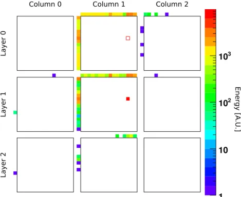
Fig. 3.5 shows a typical implantation event. In the figure, the readings from the detector strips are shown to the left and to the top of each detector; the beam enters from the top. (See fig. 2.7 for the active stopper layout.)

As can been seen, the implantation causes multiple strips to register a signal. In order to determine the implantation position more precisely, we take the strips above a certain

34

3.1 Software: R2D2

Figure 3.4: Schematic response curve of MPR-16-log Si preamplifier (taken from the manual [20]).

1 10 10

10

Energy [A.U.]

Layer 0Layer 1Layer 2

Column 0 Column 1 Column 2

Figure 3.5: Typical implantation event (see text for explanation).

3 Data analysis

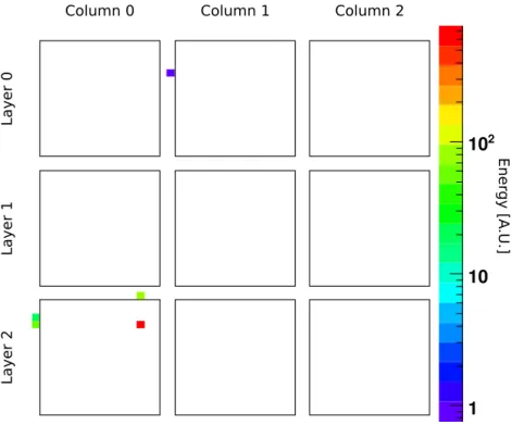
1 10 10

gy [A.U.]

Layer 0Layer 1Layer 2

Column 0 Column 1 Column 2

Figure 3.6: Decay event.

energy threshold and group them into clusters, then use the center of gravity of each cluster as the implantation position.

Obviously, implantations in the middle and end layers (layers 1 and 2) will generate shoot-through events in the preceeding layers, which need to be ignored. The algorithm simply deletes clusters which lie approximately in front of a cluster in a deeper layer.

In fig. 3.5, the filled red box indicates the implantation position as determined by the algorithm; the hollow red box corresponds to a shoot-through event which was ignored.

Fig. 3.6 shows a decay event. (The figure is oriented in the same way as fig.3.5.) As can be seen, the decay event deposits less energy and involves less detector strips, making determination of its position easier. (The very low energy seen in the middle top detector is most likely due to electronic noise.) We distinguish between implantation and decay events by the trigger type, as discussed in section 2.7.

Finally, implantation and decay events need to be matched up for implantation-decay correlation. We keep, for each pixel, a record of the most recent implantation event and the associated particle identification. If a decay event happens in that pixel, we write the particle identification to the data stream. This allows, in later analysis, to gate on the decay of a certain nucleus.

It should be noted that implantation-decay correlation is far from perfect. For the

“busy” pixels in the stopper, the average time between implantations is not necessarily small compared to the decay time. This means that more than one “active” nucleus

36