Index Overview Urban Heat Island and Outdoor Thermal Comfort for Cooling Singapore

(1)

Research Collection

Report

Index Overview Urban Heat Island and Outdoor Thermal Comfort for Cooling Singapore

Author(s):

Philipp, Conrad H.

Publication Date:

2020-08

Permanent Link:

https://doi.org/10.3929/ethz-b-000432329

Rights / License:

In Copyright - Non-Commercial Use Permitted

This page was generated automatically upon download from the ETH Zurich Research Collection. For more information please consult the Terms of use.

(2)

DELIVERABLE TECHNICAL REPORT

Version 28/08/2020

D 4.4 – Index Overview Urban Heat Island and Outdoor Thermal Comfort

Project ID NRF2019VSG-UCD-001

Project Title Cooling Singapore 1.5:

Virtual Singapore Urban Climate Design

Deliverable ID D 4.4 Index Overview Urban Heat Island and

Outdoor Thermal Comfort

Authors Conrad H. PHILIPP

DOI (ETH Collection) 10.3929/ethz-b-000432329

Date of Report 24/08/2020

Version Date Modifications Reviewed by

1 17/07/2020 Original Leslie K. Norford, Juan A. Acero, Manon Kohler, Muhammad O. Mughal

2 04/08/2020 Version 1 Ido Nevat

3 11/08/2020 Version 2 Ido Nevat, Winston T.R. Chow

4 17/08/2020 Version 3 Leslie K. Norford, Yuliya Dzyuban

(3)

Abstract

Decades of research have shown that cities are nearly always some degrees warmer than non-urban areas. This phenomenon is one of the clearest examples of inadvertent climate modification by humans.

The existence of elevated temperature on street level affects cooling needs. All of this is added to the thermal stresses on humans in hot climates or heatwave events and has prompted considerable research to mitigate aspects of urban heat in cities through urban design measures.

The report is divided into three chapters, beginning with investigation about the urban heat effect and combining the following topics

i) a historical view of the urban heat research, ii) definitions to tackle the urban heat phenomenon,

iii) consideration of four atmospheric layers to describe the spatial and temporal characteristics of urban heat, how they are caused and linked, version to measure and model them.

The second chapter deals with the urban effect on human climates. Outdoor microclimates in cities are extraordinarily diverse in space and time. A variety of tools has been developed to understand the complex relationship between humans, climate and the use of outdoor spaces. Therefore, managing the urban climate through urban planning and design solutions for the benefit of human comfort is an important goal for cities worldwide. This chapter describes

i) the variables that govern the human energy balance, ii) the options to assess thermal comfort and

iii) the summarisation of the most commonly used thermal indices.

The report will be concluded with the third chapter, which summarizes the main goals to mitigate urban heat and improve the outdoor thermal comfort.

(4)

1 Urban Heat

1.1 Introduction

As millions of people are living in cities, increased temperatures are a growing fact and concern.

Elevated temperatures in cities can be found in settlements of all sizes in all climatic regions. They arise from the introduction of artificial surfaces that are characteristic of a city and radically change the aerodynamic, radiant, thermal and moisture properties in the urban region compared to its surroundings. The evaluation of the influence of settlements on the local climate has been an important task for a long time, and the thermal environment in particular has received widespread attention because of its practical implications for urban ecology, energy use, human comfort and productivity, heat-related illness and mortality, air pollution, energy demand for air conditioning, and indirectly greenhouse gas emissions (Oke 2007; Oppenheimer et al. 2014; Roth 2013; Roth and Chow 2012;

Seneviratne et al. 2012). Urbanization and the corresponding elevated temperatures – from the local- scale heat island effect, as well as arising from larger-scale climate change – have resulted in increases of heat exposure and vulnerability to people. Due to socio-economic variations in population within cities, not everyone will have the similar capacity to prepare for, respond to, cope with, and rebound from the forecasted increases of temperatures in the future (Philipp and Chow 2020).

1.2 History

Urban climatology possesses a rich and long history beginning with LUKE HOWARD’s pioneering work.

He was a chemist, as well as, an amateur meteorologist and became most famous for his classification of clouds. In 1815, he conducted the first systematic urban climate study by means of measuring what is now called the Urban Heat Island (UHI) effect, using thermometers in the city of London and in the countryside nearby (Howard 1818). It is also remarkable that he identified virtually all responsible causes for the development of the UHI during this early study. Subsequent urban climate research replicated HOWARD’s findings from urban-rural pairs of thermometers at about 2 m height in many cities.

A large number of UHI maps generated from a thermometer measuring platform mounted on top of a vehicle to measure the different temperatures in a city (mobile traverses) appeared in the literature during the 1930s. Much of the research during this period, with a focus on German work, was summarized by the Benedictine F^ATHERA^LBERT K^RATZER in a monograph entitled “Das Stadtklima” (The Urban Climate) (Kratzer 1937), which also provided the first systematic review of the influence of settlements on air temperature. A comprehensive summary of UHI studies (maps and statistics) carried out primarily in European and North American cities was subsequently published by HELMUT LANDSBERG in his book entitled “The Urban Climate” (Landsberg 1981). During the 1970s and 1980s, the focus shifted from the largely descriptive early works toward exploring the processes responsible for the urban effect with many fundamental contributions by TIM OKE, laying the foundation for a modern treatment of this topic (Roth 2013).

(7)

1.3 Definitions

The Urban Heat concept is often used to describe ‘excess’ heat associated with urban areas, and is, therefore, frequently considered to be a negative phenomenon that requires mitigation (Martilli et al.

2020). The following explanations provide an overview of common urban heat definitions. In the absence of a standard methodology to calculate the urban heat intensity from urban to nonurban differences, different approaches will be presented as follows.

1.3.1 Urban heat Island

The Urban Heat Island (UHI) effect is the condition that describes higher temperatures in urban areas than surrounding areas of less development (Howard 1833). Care is needed in both urban and rural environments to identify representative measurement locations (Oke 2017). It cannot be assumed that the rural observations taken in the vicinity of an urban area represent pre-urban conditions. This places a particular emphasis on the selection and proper description of the rural reference site during the planning and design of a study to ensure that it is free from urban influences (Roth 2013).

1.3.2 Land use land cover comparison

Land Use Land Cover (LULC) data are a result of classifying raw satellite data (e.g. from Landsat or Aster) into LULC categories. LULC provides a very valuable method for determining the extent of various land uses and cover types, e. g., forest, shrubland and agriculture (NCSUL 2020, EOSDIS 2020). To receive information about the urban heat effect (through modelling or direct measurements) one or several rural and urban locations in different LULC types are to be compared.

1.3.3 Local climate zones comparison

The proposed Local Climate Zones (LCZ) by Stewart and Oke (2009a, 2009b, 2012) is a classification scheme to be applied for reporting of field sites (urban and rural). This system replaces the traditional and simple LULC descriptors “rural” and “urban” with more sophisticated ones, which take into account the diversity of real cities and their surroundings. The suggested LCZ are differentiated according to surface cover (built fraction, soil moisture, albedo), surface structure (sky view factor, roughness height), and cultural activity (anthropogenic heat flux). To receive information about the urban heat effect (through modelling or direct measurements) one or several rural and urban LCZ, must be compared (Roth 2013).

1.3.4 All green vs. current

Observations, either from single points or networks of stations, are supposed to represent the urban effect on the climate; however, determination of the “true” effect is in most cases not possible, because observations prior to the urban settlement do not exist. An alternative scientific approach is to hypothesize a meso-scale climatic modelling scenario replacing the urban areas from an LCLU map or LCZ map with vegetation. This hypothetical modelling scenario is termed “All Green” (Layer 2). The

(8)

difference of Layer 1 and Layer 2 is the resulting urban heat effect. Under the Cooling Singapore project the ‘all green’ vs. ‘current’ framework was applied by using simulation results of the meso-scale Weather Research and Forecasting (WRF) model with air temperature data for Singapore from April 2016 and a hypothetical scenario where Singapore is covered by vegetation (Mughal et al. 2019).

1.3.5 Urban heat footprint

The Urban Heat Footprint (UHF) effect defines a statistical framework. The UHF quantifies the urban warming at any location in the spatio-temporal domain due to different effects, i.e. active anthropogenic, passive anthropogenic and on-anthropogenic ones. To proceed with the proposed UHF framework, it is necessary to provide a probabilistic interpretation of climate models (e.g. the Weather Research and Forecasting, WRF). The UHF approach, which is model-based, assumes that the spatial-temporal temperature process is stochastic in nature. This enables to use well known and readily available approaches of estimation theory to perform inferential statistics regarding population. Under the Cooling Singapore project the UHF framework was also applied by using simulation results of the meso-scale WRF model with air temperature data for Singapore from April 2016 and a hypothetical scenario where Singapore is covered by vegetation (Nevat et al. 2020b and Mughal et al. 2019).

1.3.6 Discussion

Martilli et al. (2020) argue that the UHI intensity has little relevance for urban heat mitigation, and suggest the term “urban heat mitigation” to more accurately describe strategies aimed at cooling cities.

They proposed a shift in focus from evaluation of temperature differences between urban and rural locations to the analysis of the temperature differences within the urban areas, between zones with different urban structure, e.g. two differently built LCZ. Urban heat mitigation was taken into account in consideration of heat mitigation strategies (Acero and Ruefenacht 2017), as well as microclimatic investigations (e.g. undertaken by the Cooling Singapore project since 2017), based on the most common outdoor thermal comfort indices that are addressed in the second part of this report.

1.4 Atmospheric layers, Characteristics and Underlying Processes

Heat islands can be measured as either surface or atmospheric phenomena and a further distinction can be introduced according to the observation method. Fixed station networks produce different heat islands compared to those measured using car traverses or by the thermal response from true 3-D surface compared to the bird’s eye view for surface temperature (Oke 1995, Roth 2013). Although they are related, it is essential to distinguish between the different types because the respective processes, observations, and models will differ. (Roth 2013).

Each heat island type responds to a differing set of scales, is caused by a different mix of processes, and requires different monitoring schemes to measure it and models to simulate it. The different heat island types of atmospheric layers are summarized in Table 1-4 and also shown in Figure 1.

Individual buildings, trees, and the intervening spaces create an urban “canopy” and define the microscale, found inside the roughness sublayer (RSL), which itself is a manifestation of the small-scale

(9)

above and below ground (subsurface layer). Similar houses in a district combine to produce the local scale, which is an integration of a mix of microclimatic effects. Typical local scales extend from one to several kilometers. Plumes from individual local scale systems extend vertically and merge to produce the total urban boundary layer (UBL) over the entire city, which is a mesoscale phenomenon. During daytime, this layer is usually well mixed due to the turbulence created by the rough and warm city surface, extending to a height of 1 km or more by day, shrinking to hundreds of meters or less at night.

The UBL has typical scales of tens of kilometers and can be advected as an urban “plume” downstream from the city by the prevailing synoptic winds (Roth 2013).

Figure 1: Idealized vertical structure of the urban atmosphere over (a) an urban region at the scale of the whole city (mesoscale), (b) a land-use zone (local scale), and (c) a street canyon (microscale).

Gray-shaded areas (thick line following surface in (c)) show “locations” of the four UHI types corresponding to each scale (see Table 1-4). (Source: modified by Roth 2013).

1.4.1 Urban Canopy layer UHI

The urban canopy layer (UCL)(Figure 1b and 1c, Table 1) is located within the atmosphere below the tops of buildings and trees (e. g, in the urban canopy) and is a local (neighborhood)-scale phenomenon.

Given its accessibility and relevance to human activities, it is the most commonly studied atmospheric

(10)

volume inside the canyon, primarily through sensible heat transfer from the surface into the canyon to change the temperature (Roth 2013).

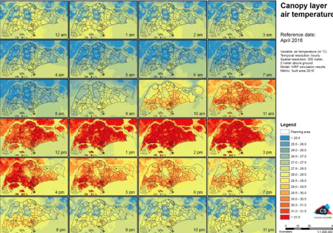
The UCL-UHI is correlated with several weather elements, but dominant are wind speed and cloud cover. The physical reason is that wind speed is a measure of atmospheric transport and mixing; the main drivers of advection and turbulent exchange that limit horizontal and vertical temperature differences. Similarly, cloud cover fraction (amount of sky obscured) and cloud type (indirectly related to height) are the main drivers of heating and cooling. Humidity and pressure are less strongly correlated. During daytime, the urban-rural difference is relatively small. The urban heat intensity increases after sunset and reaches a maximum sometime between a few hours after sunset and before sunrise. The canopy layer urban heat is therefore primarily a nocturnal phenomenon and arises from reduced cooling rates observed in the city in the late afternoon and evening compared to the non-built- up areas resulting in higher urban minimum temperatures. After sunrise, the urban area also warms up more slowly and the heat island is rapidly disappearing (Oke 1997). To investigate the canopy layer urban heat, the Cooling Singapore team used the WRF model to simulate Singapore’s average air temperature for different climatic seasons (February, April, July and October 2016). The temporal resolution was hourly; the spatial resolution was 300 meters, and the results were evaluated at 2 metres above ground. As urban scenario the built area of Singapore (2016) was selected; as rural scenario the built area was replaced by a dense tropical forest (i.e., ‘all green’). Within Figure 2 the canopy layer urban heat effect for April 2016 is illustrated. Hereby, the simulated air temperature layer based on land cover characteristics of 2016 (layer 1) was subtracted by the simulated air temperature when all built up areas of layer 1 were replaced by dense vegetation (layer 2) (see approach described under 2.4.4).

Table 1: The canopy layer: scale, underlying processes, timing and magnitude and measurement techniques to observe them (Source: Roth 2013 and Oke 1997, Oke 1982, 1995; Oke et al. 1991; Voogt 2002).

Parameter Description

Spatial location One to ten kilometres vertical

Processes Day: strong positive heat flux at surface; sensible heat flux convergence in urban canyon; Night: often positive sensible heat flux supported by release of heat from storage in ground and buildings and anthropogenic heat

Timing, temperature difference between urban and rural

Day: small, sometimes negative if extensive shading

Night: large and positive, increases after sunset, maximum between a few hours after sunset and predawn hours

Models Canopy and roughness sublayer scheme including interactions with subsurface and overlying boundary layers

Measurements Temperature sensors at fixed points, arrays and mobile

Causes Thermal properties of building and pavements, greater turbulent sensible heat flux from rougher, warmer city surface, anthropogenic heat (release due to fuel combustion and electricity, as well as, heat injected from chimneys and factory stacks), aerosol and gaseous pollutants alter radiation transmission, warmer polluted air (often more moist urban atmosphere emits more downward longwave radiation)

(11)

Figure 2: Canopy layer urban heat effect simulated for April 2016 by using the Weather Research and Forecasting (WRF) model (Sources: modified based on Mughal et al. 2019, DataGov 2020;

layout: Conrad Philipp).

1.4.2 Surface layer UHI

The surface layer UHI (SL-UHI) is defined by the temperature of the surface that extends over the entire 3D envelope of the surface (Figure 1a and 1b, Table 2). It is a surface energy balance phenomenon and involves all urban facets (i.e. horizonal and vertical surfaces). Urban surface temperatures are sensitive to the relative orientation of the surface components to the sun during day and to the sky at night, as well as to surfaces’ thermal (e.g. heat capacity, thermal admittance) and radiative (e.g.

emissivity, albedo) properties. The surface temperature difference between the built areas and the vegetated areas is highest during daytime, due to the solar irradiation of the exposed horizontal surfaces (i.e. roofs and pavements). The hottest surfaces during day-time are usually measured in industrial and commercial areas, especially in those with large roofs and pavements (e.g. airports, shopping malls, and major highway intersections) (Roth 2013). At night, some of the processes are reduced, and urban- rural differences and intra-urban variability of surface temperature are smaller than during the day (Roth et al. 1989).

To identify the SL-UHI (Figure 1a and 1b), scientists use direct and indirect methods, numerical modeling, and estimates based on empirical models. In addition researcher use remote sensing, an indirect measurement technique, to estimate the temperatures of the surface (Philipp 2019, ESA 2020, USGS 2020).

(12)

Table 2: The surface layer: scale, underlying processes, timing and magnitude and measurement techniques to observe them (Source: Roth 2013 and Oke 1997, Oke 1982, 1995; Oke et al. 1991; Voogt 2002).

Spatial location One to several hundred metres vertical

Processes Day: surface energy balance; strong radiation absorption and heating by exposed dry and dark surfaces

Night: surface energy balance, roofs – large cooling (large sky view); canyon facets – less cooling (restricted sky view)

Timing, temperature difference between urban and rural

Day: very large and positive Night: large and positive

Models Surface energy balance and equilibrium surface temperature Measurements Numerical modelling, and estimates based on empirical models

(in addition the surface temperature can be measurements through to temperature sensors mounted on satellites and aircrafts)

Causes Thermal properties of building and pavements (e.g. building materials often have greater capacity to store and later release sensible heat), greater turbulent sensible heat flux from rougher, warmer city surface, anthropogenic heat (release due to fuel combustion and electricity, as well as heat injected from chimneys and factory stacks), aerosol and gaseous pollutants alter radiation transmission, warmer polluted air (often more moist urban atmosphere emits more downward longwave radiation)

1.4.3 Urban boundary layer UHI

The urban warmth extends into the UBL (above the RSL) through convergence of sensible heat plumes from local scale areas (bottom-up) and the entrainment of warmer air from above the UBL (top-down) to create the urban boundary layer UHI (UBL-UHI). The UBL-UHI (Figure 1a, Table 3) is maintained by an enhanced sensible heat flux from the city, which promotes mixing in the lower atmosphere during daytime and sustains it overnight. As a result, the urban boundary layer is warmer than the rural one (Oke 2017). Because of experimental difficulties to probe the air at large heights, the BL-UHI has not received as much attention as its canopy layer counterpart. A few airplane, helicopter, remote sensing, balloon, and tower studies have been conducted since the 1960s in a wide range of cities. They provide insight into the vertical structure of the nocturnal urban boundary layer and confirm that the urban heat extends upward to a height of several 10s kilometres. The temperature in the boundary layer, different between urban and rural areas, is largest under light winds and when strong rural surface inversions exist, as well as, weaker for strong winds when the vertical temperature distribution is more uniform.

The boundary layer urban temperature is less compared to that measured in the canopy layer (Roth 2013).

(13)

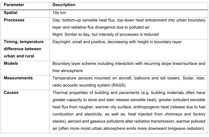
Table 3: The boundary-layer: scale, underlying processes, timing and magnitude and measurement techniques to observe them (Source: Roth 2013 and Oke 1997, Oke 1982, 1995; Oke et al. 1991; Voogt 2002).

Spatial 10s km

Processes Day: bottom-up sensible heat flux, top-down heat entrainment into urban boundary layer and radiative flux divergence due to polluted air

Night: Similar to day, but intensity of processes is reduced Timing, temperature

difference between urban and rural

Day/night: small and positive, decreasing with height in boundary layer

Models Boundary layer scheme including interaction with recurring slope linear/surface and free atmosphere

Measurements Temperature sensors mounted on aircraft, balloons and tall towers, Sodar, lidar, radio acoustic sounding system (RASS)

Causes Thermal properties of building and pavements (e.g. building materials often have greater capacity to store and later release sensible heat), greater turbulent sensible heat flux from rougher, warmer city surface, anthropogenic heat (release due to fuel combustion and electricity, as well as, heat injected from chimneys and factory stacks), aerosol and gaseous pollutants alter radiation transmission, warmer polluted air (often more moist urban atmosphere emits more downward longwave radiation)

(14)

1.4.4 Subsurface layer UHI

The subsurface layer UHI (SSL-UHI) (Figure 1a-c, Table 4) is characterized by transfer of sensible heat from the urban surface and urban infrastructure into the ground; it is warmer and more variable beneath more densely built areas and areas with little vegetation, but cooler in more vegetated areas. In cities the depth of the affected layer may be several tens, and even a hundred metres deep (Popiel et al., 2001). The subsurface soil temperature is a crucial variable to control the ecosystem’s biological and chemical processes such as soil respiration, thawing of permafrost, microbial decomposition and groundwater flow. It also has a strong impact on the underground infrastructure, especially in an urban context. There are only a few observations of subsurface temperature compared to those of the surface or the air (Menberg et al., 2013).

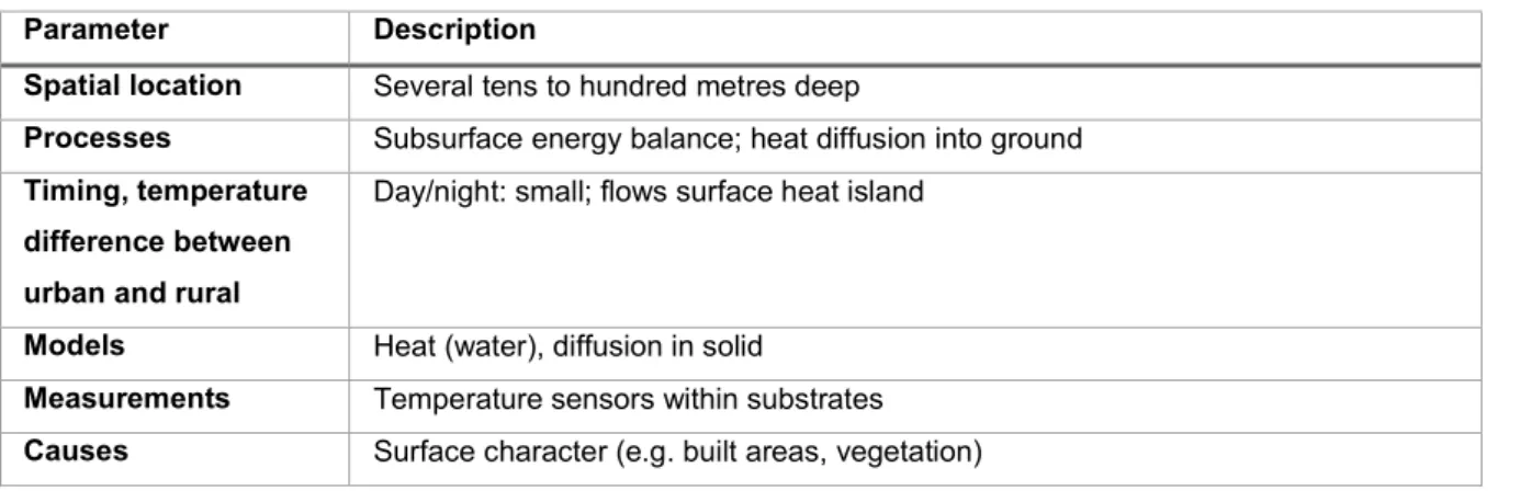
Table 4: The subsurface layer: scale, underlying processes, timing and magnitude and measurement techniques to observe them (Source: Roth 2013 and Oke 1997, Oke 1982, 1995; Oke et al. 1991; Voogt 2002).

Spatial location Several tens to hundred metres deep

Processes Subsurface energy balance; heat diffusion into ground Timing, temperature

difference between urban and rural

Day/night: small; flows surface heat island

Models Heat (water), diffusion in solid

Measurements Temperature sensors within substrates Causes Surface character (e.g. built areas, vegetation)

1.5 Methods of Analysis

Observational and modelling approaches are used to investigate the urban thermal environment. Field observations provide descriptive information about the UHI and the processes causing it, and the methods differ for each UHI type. Observations are also essential to evaluate the full range of physical (scale), statistical, or numerical models used to investigate these processes and predict urban heat behaviour (Roth 2013).

1.5.1 Observations

The spatial and temporal variability of surface temperature (see chapter 2.4.2) has been investigated using thermal infrared measurements of upwelling thermal radiance with instruments based at ground level (e.g. pyrgeometer and thermal scanner), on aircraft (e.g. thermal scanner), and on satellites (e.g.

Landsat or MODIS) (Roth 2013). The canopy layer heat island is observed using thermometers to measure air temperature near the ground. Air temperature can be measured at one or more sites considered to be representative of urban and rural conditions (WMO, 2008; Stewart and Oke, 2012).

This is called the ‘fixed’ approach. If the stations have continuous monitoring and recording equipment,

(15)

vehicle and traversed across a settlement and its surrounding non-urbanized area. This ‘traverse’

approach provides insight into small scale spatial variations of the air temperature. Fixed stations more easily reveal the temporal dynamics, whereas traverses provide insight into the spatial thermal response to variations in urban form (Oke 2017).

Figure 3: Installation of local weather stations in the Central Business District of Singapore to measure the local climatic conditions (2 m above ground) (Image: Cooling Singapore, 2020)

If the objective is to monitor the thermal environment of the canopy layer, the sensors must be exposed so that their microscale surroundings are representative of the local-scale environment of the selected neighbourhood (see Figure 3). The sensor location must be surrounded by “typical” conditions for urban terrain. Ideally, the site should be located in an open space, where the surrounding height/width ratio (H/W ratio) of the buildings is representative of the local environment, away from trees, buildings or other obstructions. Care should be taken to standardize the practice across all sites used in a network regarding radiation shields, ventilation, height (2–5 m is acceptable given that the air in canyons is usually well mixed) and to ensure that sensors are properly calibrated against each other (Roth 2013).

1.5.2 Numerical Models

Numerical models, in comparison to scale and statistical models, offer increased capabilities to simulate the full complexity and diversity of cities and their interactions with the atmosphere. They vary substantially according to their physical basis and their spatial and temporal resolution and have been developed to assess impacts of urbanization on the environment and, more recently, provide accurate meteorological information for planning mitigation and adaptation strategies in a changing climate.

(16)

Considering its central role in understanding and predicting the urban climate, including the UHI, the urban energy balance has received much attention of the modelling community (Roth 2013).

One of the first microscale models to simulate the small-scale interactions between individual buildings, ground surfaces, and vegetation was ENVI-met (Bruse and Fleer 1998). It is a nonhydrostatic model designed for the microscale dynamics with very high temporal and spatial (0.5–10 m) resolution and a typical time frame of 24–48 h, capable to simulate the diurnal cycles of temperature, thermal comfort, and many standard atmospheric variables across a realistic building array.

Mesoscale meteorological models (resolution of several hundred metres), on the other hand, are able to simulate the spatial structure and temporal dynamics of the UHI intensity across entire cities. To bridge the gap between traditional mesoscale and microscale modelling, the National Centre for Atmospheric Research (NCAR), in collaboration with other agencies and research groups, has developed an integrated urban modelling system coupled to the WRF model (e.g. Chen et al. 2011).

This urban modelling community tool includes three methods to parameterize urban surface processes, ranging from a simple bulk parameterization to a sophisticated multilayer urban canopy model with an indoor–outdoor exchange approach that directly interacts with the atmospheric boundary layer and procedures to incorporate high-resolution urban land use, building morphology, and anthropogenic heating data (Roth 2013). This WRF/urban model has been used, e.g., for high-resolution regional climate simulation of the air temperature of Singapore for four seasons in 2016 (Mughal 2019).

2 Urban effect of climate on humans

2.1 Introduction

Thermal comfort (Outdoor Thermal Comfort, OTC, as well as Indoor Thermal Comfort, ITC) is defined as the condition of mind that expresses satisfaction with the thermal environment according to subjective evaluation (Oke 2017; ASHRAE 2009). Crucially, this definition highlights the role of psychology in assessing one’s thermal state. Satisfaction with the thermal environment is important because thermal conditions are potentially life-threatening for humans, if the core body temperature reaches conditions of hyperthermia, above 37.5–38.3 °C, or hypothermia, below 35.0 °C. A comfortable individual feels neither too warm nor too cold and has no desire to either alter their clothing/activity levels or to modify the environment, to which they are exposed. The combination of environmental variables can also result in thermal stress, which causes the body to respond by experiencing strain.

Cold thermal stress causes the body to generate internal heat, while limiting heat losses. Warm thermal stress causes the body to maximize heat loss. Cold and warm thermal stress can vary greatly between individuals. Overall, the body must achieve an energy balance so that the body temperature is constant (Oke 2017). Particularly in the tropical regions, the combination of high air temperature, high humidity and prevailing low wind speed makes achieving a comfortable thermal environment very challenging (Binarti et al. 2019).

(17)

2.2 Variables

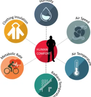
There are four climatic variables that govern the energy balance terms. They include the wind velocity, air temperature, relative humidity, as well as moisture in the air, and radiation. The latter is encapsulated by the mean radiant temperature (TMRT), which expresses the short and long wave radiation absorbed at the outer surface of the body. The terms that are intrinsic to humans are levels of activity and of clothing. All these environmental variables of relevance to humans are modified in the city. While some of these changes may be beneficial, others are deleterious (e.g. dangerous winds, poor air quality).

Urban heat raises surface and air temperatures and will lead to thermal stresses in hot climates (or weather). In general, in warm weather, low wind speed and a high relative humidity causes considerable stress to which the body responds by sweating (Oke 2017). The variables that regulate thermal stress and body strain will be explained in Table 5 and Figure 4 (WMO 2015).

Figure 4: Variables that influence human comfort (Sources: SimulationHub 2019)

Table 5: Variables that regulate thermal stress and body strain (Sources: ASHRAE 2009; Boduch and Fincher 2010; Oke 2017; Sunkpal 2015)

Metabolic rate / Activity Level (M)

The heat generated when metabolized food is chemically converted to fuel both internal (e.g.

breathing) and external (e.g. running) physical activity is termed metabolic heat. While some of this energy is expended as mechanical energy (such as walking uphill), the great majority (> 95%) is converted to heat that must be dissipated to the ambient environment. The magnitude of the metabolic rate depends strongly on the level of exertion / physical activity.

The lowest value occurs when an adult is sleeping and the highest during intense physical activity.

(18)

Clothing insolation (clo)

Exchanges between the skin surface and the atmosphere are modulated by clothing (clo), which acts as a new ‘surface’ that intervenes between the skin and the ambient environment.

Most clothing is designed to protect the body from excessive sensible heat loss and this is managed through the choice of clothing. In hot climates, the primary purpose of clothing is to protect the body from solar radiation, which is best achieved through materials with a high reflectivity.

Air temperature (Ta)

The Air Temperature (Ta) is defined as the temperature of the ambient air surrounding the occupant that defines the net heat flow between the human body and its environment.

Human bodies perform within an internal temperature range considerably narrower than external temperatures. In the process, human metabolism generates heat, which must dissipate into the surrounding air or surfaces. When surrounding temperatures are high, this process becomes more difficult and the human body may overheat or feel warm. When surrounding temperatures are low, the rate of heat loss becomes more rapid, and the human body may feel uncomfortably cold.

Mean radiant temperature (MRT)

The Mean Radiant Temperature (MRT) arises from the fact that the net transfer of radiant energy between two objects can be linearized to be proportional to their temperature difference multiplied by their capacity to radiate and absorb heat also known as their emissivity. Also, the MRT can be defined as the temperature of a uniform enclosure “with which a small black sphere at the test point” would have the same radiation transfer as it does with the real environment.

Air speed / Air velocity (v)

Air speed / Air velocity (v) defines the movement of air across the layer of skin or clothing surface area, thus convecting heat. Air velocity plays a role in the perception of thermal comfort. In hot climates, as the human body attempts to cool itself, the flow of air across the body will assist in evaporative cooling as a consequence of sweating. When the humidity of air is near saturation (i.e. near 100 % relative humidity), the air next to the sweating body may become saturated with moisture, but by moving the air next to the body away and bringing in fresh, lower humidity air, the evaporation of sweat can continue. Mechanisms of convection can further move the heat generated by metabolic processes from the skin and into the surrounding air what leads to continued cooling.

Relative humidity (RH)

Relative humidity (RH) is the ratio between the actual amount of water vapor in the air and the maximum amount of water vapor that the air can hold at that air temperature. High levels of relative humidity can work against the evaporative cooling effects of sweating and leave the body prone to over-heating. When relative humidity gets too high, discomfort develops, either due to the feeling of the moisture itself which is unable to evaporate from the skin, or due to increased friction between skin and clothing with skin moisture. When relative humidity gets too low, skin and mucous surfaces become drier, leading to complaints about dry nose, throat, eyes, and skin. Air in mine working faces is nearly saturated, with relative humidity commonly ranging from 90% to 100%. Water vapor partial pressure can be calculated from relative humidity.

(19)

2.3 Thermal Comfort and its assessment

2.3.1 Measurement

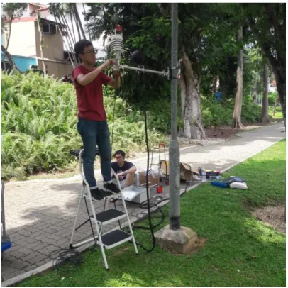
Acquiring information on outdoor human comfort is extremely difficult. Ideally one needs to gather information on radiation, wind, temperature and humidity in the environment but this is complicated due to the great number of microclimates in cities. In addition, it is necessary to link these to indicators of the biophysical and psychological response of the person, which depends on activity levels, clothing, age, health and so on. Figure 5 shows an instrument system that is designed to make climatic observations at pedestrian height. It is located in an area with public use, and a sample of people are surveyed to provide data on clothing and activity levels and their personal assessment of the thermal environment. This information may be supplemented by observations of the public use of the space (e.g. sitting/standing, preference for shade). Subsequently, this response information is correlated with the environmental data to estimate which urban design is more adequate to provide comfortable thermal conditions (Oke 2017). Cooling Singapore undertook in September 2019 a campaign to assess the thermal comfort of local Singaporean residents in a corridor park located in a mixed-use commercial and residential district (Tanjong Pagar and Duxton Plain Park).

Figure 5. Installation of the instruments for assessing thermal comfort (Image: Cooling Singapore, 2019).

(20)

2.3.2 Modelling

Numerical models of the human energy balance can simulate the thermophysical responses of the human (e.g. skin temperature and sweat rate) to environmental stimuli that change rapidly. These transient conditions require non-steady state responses. Typically, such models segment the body into parts that are represented by simpler shapes (e.g. a sphere to represent the head and cylinders of different dimensions to represent the torso, arms, legs, fingers and toes) for which view factors and exchange coefficients are known. Each segment is connected via a modelled circulatory system and the energy exchange from the core to the outer skin surface is simulated at a series of nodes that represent layers of tissue. Clothing is included as a new surface layer and the energy exchange between the node at the skin surface and that at the cloth surface is simulated. These models can be used to create rational indices of environmental stress by comparing ambient conditions against a standard (Oke 2017).

2.3.3 Thermal indices

There is a great number of thermal indicators which are based on simple measures of the environment and of thermal stresses. However, the most useful of them are based on the energy balance, which combines the exchange to physical (dis)comfort (Oke 2017). The general basis for creating human thermal climate indices is to integrate the heat-related aspects of the environment and the human body in a way that gives a simple meaning to the thermal meaning of the overall condition (Nevat et al.

2020b). Some are based on readily available meteorological data so that they have the advantage of ease of calculation; others are based on measures of thermal strain such as skin temperature or sweat rate. The most comprehensive are based on the human energy balance. For practical purposes, many of these indices are calibrated against a suite of ambient climatic, activity and clothing conditions that represent an imaginary setting, in which only air temperature is allowed to vary. The ‘equivalent’ air temperature is calculated that would exert the same stress (or cause the same strain) in these circumstances as the conditions, to which the body is currently exposed. This provides a single measure of the thermal environment (Oke 2017). The rationale for this is that most people can imagine the thermal importance of a certain air temperature based on their experience with different environmental conditions of heat and cold (Nevat et al. 2020b).

(21)

2.3.4 Historical background

Pursuing a simple index that is capable to describe human responses to the thermal environment has been done since the previous century. The first serious study on the effect of high temperature on comfort was conducted by Haldane in 1905 (Auliciems and Szokolay 1997). In the beginning of the 20th century a ‘comfortable’ environment was defined as one sensed by the occupant as neither warm nor cold. In 1923 Houghton and Yaglou tried to define the thermal comfort zone, which was then applied in the first comfort scale: Effective Temperature (ET). ET is an empirical index of stress caused by sensible and insensible heat exchange (Gagge et al. 1937) presented as a combination of air temperature and humidity in a diagram of wellness. It describes the relative effect of air temperature and humidity on comfort, but it does not take personal factors into account. The ET of an environment is equivalent to the temperature of an environment, at which the human body cannot exchange energy with the environment. Such condition is characterized by uniform temperature and stationary air with 100%

moisture content (Fabbri 2015). However, Yaglou in 1947 and Glickman et al. in 1950 found that ET overestimates the effect of humidity under cool and comfortable conditions (Auliciems and Szokolay 1997).

In 1932 air velocity was included in the diagram of wellness, while Vernon added the effect of radiation by substituting globe temperature values for a dry bulb temperature scale. The revision is called Corrected Effective Temperature (CET) nomogram (Auliciems and Szokolay 1997). In 1971 Gagge et al. introduced a simple model of the human physiological regulatory response on the ET scale based on an analytical study. This index considers clothing, activity and radiation exchange, and is presented as a series of nomograms (Fabbri 2015). In 1995 Smith discovered that in hot environments, CET underestimates the effect of humidity and overestimates the opposed effect of 0.5–1.5 m/s air velocity (Auliciems and Szokolay 1997).

Following ET, several thermal indices with a linear equation approach have been established. Yaglou and Minard (1957) developed the Wet Bulb Globe Temperature (WBGT), which indicates the combined effect of air temperature (Ta), low-temperature radiant heat, solar radiation (G), and air movement (v).

It also provides a calculation for outdoor use: the weighted average of dry bulb temperature, naturally ventilated wet bulb temperature (Twb) and globe temperature (Tg). The equatorial comfort index (ECI) developed by Webb in 1959 was intended for equatorial (warm-humid) climates, especially Malaysia and Singapore. This index was derived from 393 sets of observations of subjective responses of acclimatized subjects involved in light sedentary work (Binarti et al. 2019).

Over the last decades complete heat budget models where developed that take all mechanisms of heat exchange into account. Input variables include air temperature, water vapour pressure, wind velocity, mean radiant temperature including solar radiation, in addition to metabolic rate and clothing insulation.

Such models hypothesise to possess the essential attributes of an operational use in most biometeorological applications for all climates, regions, seasons and scales. This is certainly true for MEMI (Höppe 1984, 1999), and the Outdoor Apparent Temperature (Steadman 1984, 1994). However, it would not be the case for the simple Indoor AT, which is the basis of the US Heat Index, often used in outdoor applications neglecting the addition "Indoor". Other good indices include the Standard

(22)

Predictive Index of Human Response approach (Gagge et al. 1986). So does Out_SET* (Pickup and de Dear 2000; de Dear and Pickup 2000), which is also based on Gagge's work. Blazejczyk (1994) presented the Man-Environment Heat Exchange model MENEX, and the extensive work of Horikoshi et al. (1995, 1997) resulted in a Thermal Environmental Index. With the improvement by Gagge et al.

(1986) in the description of latent heat fluxes by the introduction of PMV*, Fanger's (1970) approach can also be considered among the advanced heat budget models. This approach is generally the basis for the operational thermal assessment procedure Klima-Michel-model (Jendritzky et al. 1979;

Jendritzky et al. 1990) of the Deutscher Wetterdienst with the outcome "perceived temperature, PT"

(Staiger et al. 1997) that considers a certain degree of adaptation by various clothing (Jendritzky et al.

2002).

2.3.5 Selected thermal indices

The many indices that have been suggested can be categorized into three groups: “rational indices”,

“empirical indices” and “direct indices”. Rational indices are based upon calculations involving the heat balance equation; empirical indices are based on establishing equations for the physiological responses of human subjects (e.g. sweat loss); and direct indices are based on the (usually temperature) measurement by means of instruments and used to simulate the response of the human body (Epstein and Moran 2006).

We have identified a total of six most commonly used thermal indices in the mentioned groups:

 rational indices: PET, mPET, OUT_SET*, UTCI,

 empirical indices: TSI,

 direct indices: WBGT.

(23)

2.3.5.1 Physiological equivalent temperature (PET)

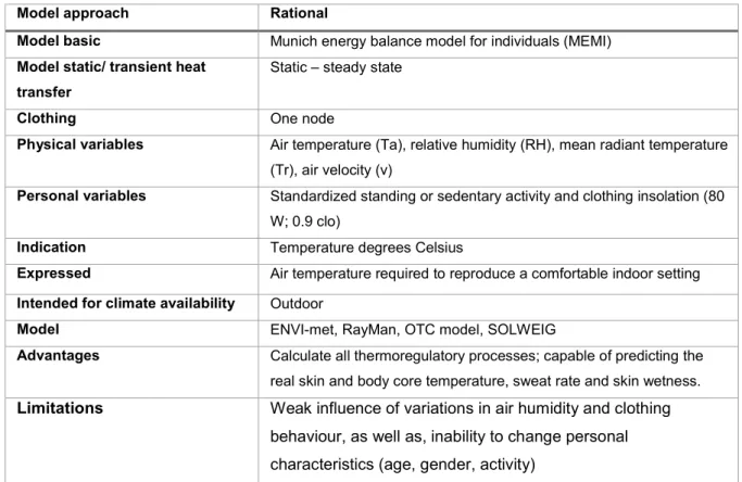
Developed specifically for outdoor environments the Physiologically Equivalent Temperature (PET, Table 6) is the air temperature required in an outdoor environment to reproduce a standardized indoor setting, for a standardized individual. This is the air temperature required to balance the heat budget of the human body with the skin and core temperatures in complex outdoor conditions (Höppe 1999, Matzarakis and Amelung 2008). The calculation of PET is based on four meteorological variables, as well as, standardized clothing and activity values (Höppe 1999, 1984). Here, the norm individual is assumed to have a work metabolism of 80 W due to light activity, in addition to basic metabolism and 0.9 coverage of heat resistance from clothing (Matzarakis and Amelung 2008). The indoor reference climate is based on the following: mean radiant temperature equals air temperature, air velocity (wind speed) is fixed at v = 0.1 m/s, and water vapour pressure is set to 12 hPa (approximately equivalent to a relative humidity of 50% at 20°C). The thermal conditions of the body are then calculated using the Munich energy balance model for individuals (MEMI), which are substituted on the other hand in the energy balance equation system to produce the PET air temperature value (Walls et al. 2015).

Currently, PET is the most frequently used thermal comfort index (Chen and Matzarakis 2014; Coccolo et al., 2016; Johansson et al., 2014), especially in hot-humid regions (Binarti et al. 2019). Since 2017 PET has been used in the Cooling Singapore project within the micro climate model ENVI-met (Pignatta et al. 2018).

Table 6: Physiological equivalent temperature (PET) (Source: Binarti et al. 2019; Chen and Ng 2012; Davis et al.

2006; Fanger 1970; Johansson et al. 2014; Rose et al. 2010; Spagnolo and De Dear 2002; Steadman 1984; Walls et al. 2015)

Model approach Rational

Model basic Munich energy balance model for individuals (MEMI) Model static/ transient heat

transfer

Static – steady state

Clothing One node

Physical variables Air temperature (Ta), relative humidity (RH), mean radiant temperature (Tr), air velocity (v)

Personal variables Standardized standing or sedentary activity and clothing insolation (80 W; 0.9 clo)

Indication Temperature degrees Celsius

Expressed Air temperature required to reproduce a comfortable indoor setting Intended for climate availability Outdoor

Model ENVI-met, RayMan, OTC model, SOLWEIG

Advantages Calculate all thermoregulatory processes; capable of predicting the real skin and body core temperature, sweat rate and skin wetness.

Limitations Weak influence of variations in air humidity and clothing behaviour, as well as, inability to change personal characteristics (age, gender, activity)

(24)

2.3.5.2 Modified Physiologically Equivalent Temperature (mPET)

Lin and Matzarakis (2008) developed the Modified Physiologically Equivalent Temperature (mPET, Table 7), as a new thermal comfort range for Taiwan. mPET can be applied in other hot-humid regions and improves the ability of PET to predict the effects of humidity on the thermal sensation (Lin et al.

2018). Furthermore, mPET provides a better way to consider the heat transfer from the inner body to the outer body. The multi-layer clothing model adopted in mPET considers the influence of clothing on latent heat transfer and includes simulations of water vapor resistance (Chen and Matzarakis, 2017).

By considering the air gap between two clothing layers, a multi-layer clothing model can produce results that are close to experimental data (Das et al. 2011; Puszkarz and Krucińska 2016) and data from surveys conducted in hot-humid regions (Lin et al. 2018; Binarti et al. 2019).

Table 7: Modified Physiological equivalent temperature (mPET) (Source: Binarti et al. 2019; Chen and Ng 2012;

Davis et al. 2006; Fanger 1970; Johansson et al. 2014; Rose et al. 2010; Spagnolo and De Dear 2002; Steadman 1984; Walls et al. 2015)

Model basic Multi-element HTM

Model static/ transient heat transfer

Dynamic – steady state and transient

Clothing 1–3 layers, 4–8 nodes clothing model

Personal variables Metabolic heat power (M) and clothing insolation (clo)

Indication Temperature degrees Celsius

Expressed Air temperature required to reproduce a comfortable indoor setting Intended for climate availability Outdoor

Model RayMan

Advantages Calculate all thermoregulatory process; improvement of the weak variance due to the changing of the relative humidity and the clothing

Limitations -

(25)

2.3.5.3 Outdoor Standard Effective Temperature (OUT_SET*)

Developed for indoor environments, the Standard Effective Temperature (SET*) is a model for calculating the dry-bulb temperature which relates the real conditions of an environment to the (effective) temperature assuming standard clothing, metabolic rate and 50% relative humidity, as well as, (Walls et al. 2015) wind speed lower than 1.5 m/s. For this thermal comfort index, air temperature is set equal to mean radiant temperature, where a person (standard clothing according to metabolic activity) has the same heat stress (skin temperature, Tsk) and thermoregulatory strain (skin wettedness, w) as in the actual environment (Blazejczyk et al. 2013; Coccolo et al. 2016). However, this model considers only the heat transfer from the inner body to the outer body by means of blood circulation (Gagge et al. 1986). Hence, the performance of SET* in situations with changing convective and radiant heat exchange is limited, and its application is appropriate only for indoor conditions (Chen and Matzarakis 2017; Binarti et al. 2019).

SET* has been modified to OUT_SET*, (Table 8), which simplifies the complex mean outdoor radiant temperature conditions to a mean radiant temperature with all other variables maintained as in SET*

(Pickup and de Dear 2000; Jendritzky et al. 2012). OUT_SET* is considering the detailed radiative exchange through a specific model (OUT-MRT), where OUT-MRT is an approximated amount of solar radiation absorbed by the human body. OUT_SET* has found a wide application in hot-humid regions (Johansson et al. 2017; Zhao et al. 2016; Jeong et al. 2016; Watanabe et al. 2014; Xi et al. 2014).

Table 8: Outdoor Standard Effective Temperature (OUT_SET*) (Source: Binarti et al. 2019; Chen and Ng 2012;

Davis et al. 2006; Fanger 1970; Johansson et al. 2014; Rose et al. 2010; Spagnolo and De Dear 2002; Steadman 1984; Walls et al. 2015)

Model basic Two-node model

Model static/ transient heat transfer

transient

Clothing not considered

Indication Temperature Degrees Celcius

Expressed Compares individual physiological comfort to a reference environment Intended for climate availability In- and Out-door

Model RayMan

Advantages Can use actual and observed values of clothing insulation and metabolic rate.

Limitations Performance on the changing of convective and radiant heat exchange

(26)

2.3.5.4 Thermal Sensation Index (TSI)

The Thermal Sensation Index (TSI) was developed for research in Japan by means of formalized testing of subjects positioned in outdoor environments for set periods of time. Subjects were asked to complete a questionnaire of thermal sensation indicating discomfort, neutral and pleasurable conditions. These experiments were conducted under various air temperature, solar and wind conditions to quantify the experience of outdoor climatic variables in relation to the subject’s experience (Walls et al. 2015).

Analysis of the experimental findings led to the development of an equation expressing thermal sensation as a function of five variables including surface temperatures of surrounding materials and

humidity (Givoni et al., 2003) (Walls et al. 2015). The TSI (Table 9) determines a measure between 0 and 7, with 4 as the most comfortable condition (Givoni et al., 2003).

Cooling Singapore undertook in September 2019 a campaign to assess the thermal comfort of local Singaporean residents, applying the TSI, in a corridor park located in a mixed-use commercial and residential district (Tanjong Pagar and Duxton Plain Park).

Table 9: Thermal Sensation Index (TSI) (Source: Binarti et al. 2019; Chen and Ng 2012; Davis et al. 2006; Fanger 1970; Johansson et al. 2014; Rose et al. 2010; Spagnolo and De Dear 2002; Steadman 1984; Walls et al. 2015)

Model approach Empirical

Model basic Thermal sensation votes of people Model static/ transient heat

transfer

Dynamic – steady state

Personal variables Seating with a moderate working, walking with normal speed; tropical clothing (0.5–0.7 clo)

Indication Scale between 0 to 7 where 4 is neutral, temperature: Degrees Celcius

Expressed Quantifies discomfort

Intended for climate availability Outdoor Tropics

Model -

Advantages Simple to use

Limitations Generated from regression of only 300 persons with R2 < 0.85; no validation

(27)

2.3.5.5 Universal Thermal Climate Index (UTCI)

In 2000, the Universal Thermal Climate Index (UTCI, Table 10) was developed by a commission established by the International Society of Biometeorology. The primary aim was to create a thermal climate index related to heat stress that would be accurate in all climates, seasons and scales, as well as, independent of personal characteristics, e.g. age, gender, specific activities and clothing (Jendritzky et al. 2012). The UTCI is based on the equivalent ambient temperature of a reference environment (Ta=Tr). The air velocity is 0.5 m/s at 10m height with 50% relative humidity at a constant water vapor pressure of 20 hPa and a metabolic rate of walking at a speed of 1.1 m/s (135 W/m²), which produces the same physiological response in a reference person, i.e. a human body model with a body surface area of 1.85 m², a body weight of 73.4 kg and body fat content at 14% (Fiala et al. 2001; Katić et al.

2016), as the actual environment. The multi-node model has been augmented with a static clothing insulation model, adjusted to ambient temperature and considering seasonal clothing adaptation habits (Blazejczyk et al. 2013; Fiala et al., 2012). The augmented model also considers the influence of changing wind speed and body movement on clothing insulation, vapor resistance and surface air layer insulation, which further affect the physiological response (Blazejczyk et al. 2013; Johansson et al.

2014). As mentioned above, the metabolic rate is set to 135 W/m², which is higher than the metabolic rate of the same activity in humid tropic regions (Johansson et al. 2014). This limitation may restrict the application of UTCI in hot-humid regions (Binarti et al. 2019).

Table 10: Universal Thermal Climate Index (UTCI) (Source: Binarti et al. 2019; Chen and Ng 2012; Davis et al.

Model approach Direct indices

Model basic Passive and active system – multi-node (Fiala) HTM Model static/ transient heat

transfer

Dynamic – steady state and transient

Clothing Multi-node static clothing model

Personal variables Metabolic heat power (M) = 135 W/m², walking speed 1.1 m/s and clothing insolation (clo)

Indication Indication of physiological thermal stress under a wide range of conditions and climates

Intended for climate availability Outdoor Tropics

Model ENVI-met, RayMan, OTC model, SOLWEIG, UTCI calculator Advantages Very sensitive to the changes of temporal Tr and v

Limitations Does not consider the influence of specific clothing behaviour on the thermal responses; restricted applications for some extreme thermal

(28)

2.3.5.6 Wet-bulb globe temperature (WBGT) Index

So far, the wet-bulb globe temperature (WBGT, Table 11) has been the most widely used thermal climate index throughout the world. This thermophysical index was developed in the US Navy as part of a study on heat related injuries during military training. The WBGT index measures heat stress of an individual under direct sunlight (Chow et al. 2016), which emerged from the “corrected effective temperature” consists of weighting of dry-bulb temperature (Ta) wet-bulb temperature (Tw) and black- globe temperature (Tg). The coefficients in this index were determined empirically. But, it was found that heat casualties and the time lost due to cessation of training in the heat were both reduced by using this index that is recommended by many international organizations for setting criteria for exposing workers to hot environment (Epstein and Moran 2016).

Table 11: Wet-bulb globe temperature (WBGT) Index (Source: Binarti et al. 2019; Chen and Ng 2012; Davis et al.

Model approach Direct indices (Linear equation) Model basic Three analysis of microclimate conditions Model static/ transient heat

transfer

static

Indication Apparent temperature

Intended for climate availability In- and Out-door

Model Equation

Advantages A well-established standard

Limitations Overestimates heat stress in hot climates

(29)

2.4 Outdoor thermal comfort evaluation

Outdoor thermal comfort evaluation identifies the comfortable or acceptable thermal conditions for local residents, to understand human body perception of the thermal environment, and to provide valuable reference for urban planners and decision makers, so as to formulate strategies for optimizing the outdoor thermal environment. To definitively assess a design in terms of microclimate, it is important to consider the thermal comfort of space for the entire period of use as opposed to just a point in time.

This is met by the Outdoor Thermal Comfort Autonomy (OTCA), which is an organized way of presenting spatiotemporal variation of any index. OTCA is a metric used to describe the percentage of occupied times of the year during which a designated area meets a set of thermal comfort acceptability criteria. These upper and lower bounds can be defined by PET or UTCI assessment scales. For example, an OTCA calculation based on PET would count the duration for which a space is between 18 and 23 °C PET (equivalent to no thermal stress). Spatial Outdoor Thermal Comfort Autonomy (sOTCA) forms the basis for the rapid and comprehensive assessment of outdoor space and offer a simplified means to track the incremental improvement of design (Nazarian et al. 2019).

3 Solutions to mitigate urban heat and improve the outdoor thermal comfort

Cities and their populations will continue to grow, increase stress on local environments, and remain important drivers of global environmental change. A good understanding of the nature of urban warming is important to

 inform the construction of models to provide predictions to assess impacts on human comfort and mortality (Philipp and Chow 2020),

 Understand heat related illnesses or morbidity

 provide sound planning tools to assess the net impact of climate-based interventions for the design of more sustainable cities (Chan 2020, Nevat et al. 2020b), and

 explore the intimate relationship between the urban heat and energy use and demand in cities and, hence, greenhouse gas emissions, which contribute to anthropogenic climate change.

(Acero und Ruefenacht 2017; Chow and Roth 2006; Oke 2006; Roth 2007; Smith et al. 2014).

At this point the Cooling Singapore project should be highlighted which undertake urban climate research in the tropical high-density city of Singapore, where urban warming is a timely problem (Chow and Roth 2017).

Cooling Singapore is a multi-institutional initiative established by the Singapore-ETH Centre since 2017.

The initiative addresses the urban heat challenge, which could lead to elevated heat stress and

(30)

and the well-being and productivity of its residents. This interdisciplinary team works with stakeholders including government agencies and citizens, making the process of developing guidelines and policies to mitigate urban warming inclusive and collaborative.

This initiative supports planners and policy-makers by developing integrated approaches to mitigate urban warming by combining the best of climate science, engineering and social science to develop viable strategies. In detail, the initiative aims to: (1) assess the impacts and risks of urban warming to Singapore’s economy, environment and society, and (2) develop actionable design and planning guidelines to support urban planners in urban heat mitigation and adaptation. Cooling Singapore studies the urban heat problem in a holistic manner by combining state-of-the-art urban climate modelling techniques, energy systems simulation, on-site measurements, satellite-based remote sensing, and survey campaigns.

The team has developed a range of outputs to support decision making by policy-makers in Singapore (Chan 2020, Nevat et al. 2020b).

First, the team has classified and quantified the sources of anthropogenic heat emission in an energy flow diagram (known as Sankey diagram, Kayanan et al. 2019) in order to identify the sectors that contribute most to urban warming (Fonseca and Ivanchev 2020, Kayanan 2020).

Second, climate modelling techniques are employed to produce a heat map to visualise the spatial- temporal evolution of urban warming (Mughal et al. 2019, Ayu Sukma et al. 2020, Acero et al. 2019b, Chew et al. 2020) in order to understand where and when the problem is most pronounced. Third, the team has produced a catalogue of 86 urban heat mitigation measures, ranging from vegetation, urban geometry, water bodies, materials, shading, transport and energy systems (Acero and Ruefenacht 2017, Acero et al. 2019a).

Fourth, by coupling climate modelling results with on-site measurements, the team was able to perform quantitative assessment in the form of what-if-scenarios, including measures such as innovative transportation systems, advanced building technologies, and climate-sensitive urban design solutions.

In addition to providing technical support tools, the team evaluated the socio-economic benefit of proposed measures. In a series of survey campaigns, citizens expressed their preference and willingness to pay for mitigation measures by ranking a set of proposed measures for their neighbourhood (Borzino et al. 2020). A field experiment on the cognitive performance of older adults under different climate exposures was conducted to assess the impact of urban heat on elderly residents.

Fifth, a spatio-temporal vulnerability analysis to identify areas of the city where heat exposure and sensitivity of the population are particularly high. The vulnerability analysis follows the latest definition of the International Panel on Climate Change (IPCC). The UHV index (Urban Heat Vulnerability) is used to measure the effects of physical exposure, demographic sensitivity and socio-economic adjustment parameters. Physical exposure parameters such as: air temperature, humidity and vegetation coverage were examined. Also, socio-economic adaptive capacity parameters such as: age, unemployment, outdoor occupation, and accessibility to medical services and air-conditioned facilities

(31)

were considered. The various parameters were equally weighted and spatially overlaid to determine the respective levels of risk of an urban area. A total of 28 planning areas were assessed, covering 98.8% of the population and 44 % of Singapore’s land area. The areas with high UHV are defined as risk areas or hotspots. As a result of the vulnerability analysis, the planning areas are summarized into three hotspots in the coolest hour of the day (at 7 am) and five hotspots in the hottest hours of the day (from 2 pm to 4 pm). The findings help to define areas where heat mitigation measures are needed most, in order to ensure the protection of the population (Philipp and Chow 2020).

Currently, the Cooling Singapore team is developing guidelines as well as a decision support system that will allow policy-makers to take urban climate into consideration at early stages of the planning and urban design process.

4 Acknowledgment

The research was conducted under the Cooling Singapore project, funded by Singapore’s National Research Foundation (NRF) under its Virtual Singapore programme. Cooling Singapore is a collaborative project led by the Singapore-ETH Centre (SEC), with the Singapore-MIT Alliance for Research and Technology (SMART), TUMCREATE (established by the Technical University of Munich), the National University of Singapore (NUS), the Singapore Management University (SMU), and the Agency for Science, Technology and Research (A*STAR).

5 References

Acero, J.A., E.J.Y. Koh, X.X. Li, L.A. Ruefenacht, G. Pignatta, and L.K. Norford, 2019a: Thermal impact of the orientation and height of vertical greenery on pedestrians in a tropical area, Building Simulation, 12, pp. 973–984, DOI: 10.1007/s12273-019-0537-1.

Acero, J.A., E.J.Y. Koh, G. Pignatta, and L.K. Norford, 2019b: Clustering weather types for urban outdoor thermal comfort evaluation in a tropical area, Theoretical and Applied Climatology, 139, pp.

659-675, DOI: 10.1007/s00704-019-02992-9.

Acero, J., and L.A. Ruefenacht, 2017: Strategies for Cooling Singapore: A catalogue of 80+ measures to mitigate urban heat island and improve outdoor thermal comfort, ETH Zurich Research Collection, 96 pp, DOI: 10.3929/ethz-b-000258216.