RELATING PHASE FIELD AND SHARP INTERFACE APPROACHES TO STRUCTURAL TOPOLOGY OPTIMIZATION

DOI:10.1051/cocv/2014006 www.esaim-cocv.org

RELATING PHASE FIELD AND SHARP INTERFACE APPROACHES TO STRUCTURAL TOPOLOGY OPTIMIZATION

Luise Blank

, Harald Garcke

, M. Hassan Farshbaf-Shaker

and Vanessa Styles

Abstract. A phase field approach for structural topology optimization which allows for topology changes and multiple materials is analyzed. First order optimality conditions are rigorously derived and it is shownviaformally matched asymptotic expansions that these conditions converge to classical first order conditions obtained in the context of shape calculus. We also discuss how to deal with triple junctions wheree.g.two materials and the void meet. Finally, we present several numerical results for mean compliance problems and a cost involving the least square error to a target displacement.

Mathematics Subject Classification. 49Q10, 74P10, 49Q20, 74P05, 65M60.

Received March 8, 2013. Revised January 10, 2014.

Published online August 5, 2014.

1. Introduction

In structural topology optimization one tries to distribute a limited amount of material in a design domain such that an objective functional is minimized. Known quantities in these problems aree.g.the applied loads, possible support conditions, the volume of the structure and possible restrictions as for example prescribed solid regions or given holes.A priori the precise shape and the connectivity (the “topology”) of the structure is not known. Often also the problem arises that several materials have to be distributed in the given design domain.

Different methods have been used to deal with shape and topology optimization problems. The classical method uses boundary variations in order to compute shape derivatives which can be used to decrease the objective functional by deforming the boundary of the shape in a descent direction, seee.g.[41,53,54] and the references therein. The boundary variation technique has the drawback that it needs high computational costs and does not allow for a change of topology.

Keywords and phrases.Structural topology optimization, linear elasticity, phase-field method, first order conditions, matched asymptotic expansions, shape calculus, numerical simulations.

1 Fakult¨at f¨ur Mathematik, Universit¨at Regensburg, 93040 Regensburg, Germany.luise.blank@mathematik.uni-regensburg.de;

harald.garcke@mathematik.uni-regensburg.de

2 Weierstrass Institute for Applied Analysis and Stochastics, Mohrenstrasse 39, 10117 Berlin, Germany.

Hassan.Farshbaf-Shaker@wias-berlin.de

3 Department of Mathematics, University of Sussex, Brighton, BN1 9QH, UK.v.styles@sussex.ac.uk

Article published by EDP Sciences c EDP Sciences, SMAI 2014

ET AL.

Sometimes one can deal with the change of topology by using homogenization methods, see [2] and variants of it such as the SIMP method, see [7] and the reference therein. These approaches are restricted to special classes of objective functionals.

Another approach which was very popular in the last ten years is the level set method which was originally introduced in [45]. The level set method allows for a change of topology and was successfully used for topology optimization by many authors, seee.g.[17,44]. Nevertheless for some problems the level set method has diffi- culties to create new holes. To overcome this problem the sensitivity with respect to the opening of a small hole is expressed by so called topological derivatives, see [54]. Then, the topological derivative can be incorporated into the level set method, seee.g.[18], in order to create new holes.

The principal objective in shape and topology optimization is to find regions which should be filled by material in order to optimize an objective functional. In a parametric approach this is done by a parametrization of the boundary of the material region and in the optimization process the boundary is varied. In a level set method the boundary is described by a level set function and in the optimization process the level set function changes in order to optimize the objective. As the boundary of the region filled by material is unknown the shape optimization problem is a free boundary problem. Another way to handle free boundary problems and interface problems is the phase field method which has been used for many different free boundary type problems, see e.g.[20,23].

In structural optimization problems the phase field approach has been used by different au- thors [9,11,12,16,24,50,55,58–61]. The phase field method is capable of handling topology changes and also the nucleation of new holes is possible, see e.g. [9]. The method is applied for domain dependent loads [11], multi-material structural topology optimization [60], minimization of the least square error to a target dis- placement [55], topology optimization with local stress constraints [18], mean compliance optimization [9,55], compliant mechanism design problems [55], eigenfrequency maximization problems [55] and problems involving nonlinear elasticity [50].

Although many computational results on phase field approaches to topology optimization exist there has been relatively little work on analytical aspects. One result to be mentioned is the Γ-convergence result, see e.g.[11], which relates the phase field energy in topology optimization to classical objective functionals. There is an existence result for the phase field model for compliance shape optimization in nonlinear elasticity in [50].

Most other authors derived first order conditions in a formal way and presented numerical examples obtained by a gradient flow method leading to either an Allen−Cahn [9] or a Cahn−Hilliard type phase field equation [24,55,60]. We also like to mention that in [16] a primal-dual interior point method is used to solve the phase field topological optimization problem.

Although in principle the phase field approach can also be applied for other problems in topology optimization we focus on applications formulated in the context of linear elasticity. In the simplest situation given a working or design domain Ω with a boundary∂Ω which is decomposed into a Dirichlet partΓD, a non-homogeneous Neumann partΓg and a homogeneous Neumann partΓ₀and body and surface forcesf andgone tries to find a domainΩ^M ⊂Ω(M stands for material) and the displacement usuch that the mean compliance

Ω^M

f·u+

Γ_g∩∂Ω^M

g·u

or the error compared to a target displacementuΩ,i.e.

Ω^M

c|u−u_Ω|² ν

, ν∈(0,1]

is minimized, wherecis a given weighting function and|·|is the Euclidean norm. In the paper of Allaireet al.[3]

besides other choices the case ν = ¹₂ was considered and the case ν = 1 leads to a least square minimization problem. This is the reason why we consider a range of possible choices for ν. Later we add the perimeter functional to the functional and then the minima will depend onν. Here the displacementuis the solution of

the linearized elasticity system

−∇ ·

C^ME(u)

=f in Ω^M

subject to appropriate boundary conditions. As discussed in [3] the above minimization problem is not well-posed on the set of all possible shapes and typically a perimeter regularization is used,i.e. one adds

P(Ω^M) =

(∂Ω^M)∩Ω

ds to the above functionals, where dsstands for the surface measure.

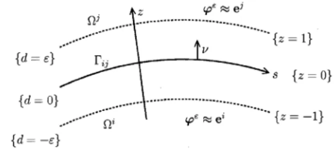
In a phase field model the domains with material and the void are described by a phase fieldϕwhich attains two given values. Moreover the interface between the domains is not sharp any longer but diffuse where the thickness of the interface is proportional to a small parameterε. The phase field rapidly changes in an interfacial region. Then the perimeter is approximated by a suitable multiple of

Ω

ε

2|∇ϕ|²+1 εΨ(ϕ)

,

where Ψ is a potential function attaining global minima at given values ofϕ which correspond to void and material. We refer to the next section for a precise formulation of the problem.

In this paper we first give a precise formulation of the problem also in the case of multi-material structural topology optimization (Sect. 2). In this context we use ideas introduced in [30,60]. Then we rigorously derive first order optimality conditions (Sect. 4). In Section 5 we consider the sharp interface limit of the first order conditions,i.e.we take the limitε→0 and therefore the thickness of the interface converges to zero. We obtain limiting equations with the help of formally matched asymptotic expansions and relate the limit, which involve classical terms from shape calculus, transmission conditions and triple junction conditions, to the shape calculus of [3].

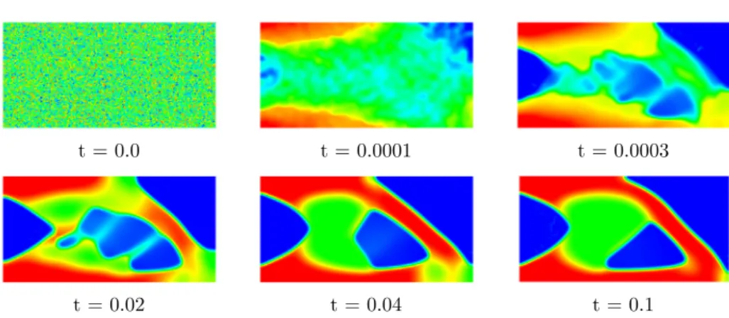
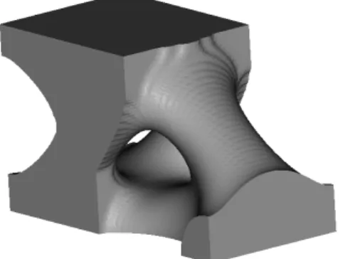
Finally we present several numerical computations by using a gradient descent method based on a vol- ume conservingL²-gradient flow of the energy. The resulting problem is a generalized non-local vector-valued Allen−Cahn variational inequality coupled to elasticity. We solve this evolution equation using a primal dual active set method as in [8].

2. Formulation of the problem

In this subsection we first introduce the phase field method and after that we will formulate the structural topology optimization problem in the phase field context.

2.1. Phase field approach

Given a bounded Lipschitz design domainΩ⊂R^d we describe the material distribution with the help of a phase field vector ϕ:= (ϕⁱ)^N_i=1, where each component ofϕ stands for the fraction of one material. Hence,d denotes the dimension of our working domainΩandN stands for the number of materials. Moreover we denote byϕ^N the fraction of void. We consider systems in which the total spatial amount of phases are prescribed,e.g.

we have additionally the constraint

−Ωϕ=m= (mⁱ)^N_i=1, wheremⁱ∈(0,1) for i∈ {1, . . . , N}is a fixed given number. We use the notation

−Ωf(x)dx := _|Ω¹_|f(x)dxwith |Ω| being the Lebesgue measure ofΩ. To ensure that all phases are present we require 0< mⁱ <1 and

N i=1

mⁱ = 1, where the last condition makes sure that N

i=1

ϕⁱ= 1 can be true. We define R^N₊ :={v ∈R^N |v ≥0}, where v≥0meansvⁱ ≥0 for alli∈ {1, . . . , N}, the affine hyperplane

Σ^N := v∈R^N | N i=1

vⁱ= 1

,

ET AL.

and its tangent plane

T Σ^N := v∈R^N | N

i=1

vⁱ= 0

.

With these definitions we obtain as the phase space for the order parameterϕthe Gibbs simplexG=R^N₊∩Σ^N. We furthermore define G := {v ∈ H¹(Ω,R^N) | v(x) ∈ Ga.e. inΩ} and G^m := {v ∈ G |

−Ωv = m}. As discussed in the introduction we use the well-known Ginzburg–Landau energy

E^ε(ϕ) :=

Ω

ε

2|∇ϕ|²+1 εΨ(ϕ)

, ε >0, (2.1)

which is an approximation of the weighted perimeter functional. The choice of E^ε as an approximation of surface energy goes back to van der Waals [57] and was also used by Cahn and Hilliard [19] in order to derive the Cahn−Hilliard equation. In minimization problems the term ¹_εΨ(ϕ) requires thatϕattains values close to the global minima ofΨ. If several global minima ofΨ exist the functionϕpossibly jumps between the minima.

It turns out that without the gradient term there is no restriction on the size of the jump set. However, the term

ε

2|∇ϕ|²penalizes interfacial regions and therefore the size of the jump set. Hence the overall functional can be interpreted as an approximation of interfacial area. In fact Modica [40] for the scalar case and later Baldo [4]

for the vector-valued case were able to show that the functional E^ε converges to the perimeter functional.

The convergence theory of the Ginzburg–Landau energy E^ε for ε→0 relies on the notion of Γ-convergence, see [4,40].

In (2.1) the functionΨ :R^N →R∪ {∞}is a bulk potential with aN-well structure onΣ^N,i.e. with exactly N global minimaei(i∈ {1, . . . , N}) and heightΨ(ei) = 0, whereei is theith unit vector inR^N. In this paper we use obstacle functionals of the formΨ(ϕ) =Ψ₀(ϕ) +I_G(ϕ), whereΨ₀∈C^1,1(R^N,R) andI_G is the indicator function ofG,i.e.

I_G(ϕ) :=

0 forϕ∈G,

∞ otherwise.

Prototype examples forΨ₀ are given by Ψ₀(ϕ) := 1

2(1−ϕ·ϕ) and Ψ₀(ϕ) := 1

2ϕ· Wϕ, (2.2)

whereW is a symmetricN×N matrix [10,25] with zeros on the diagonal which in addition is negative definite onT Σ^N. OnΣ^N we have (1−ϕ·ϕ) =ϕ·(1⊗1−Id)ϕwith1= (1, . . . ,1)^T and hence onΣ^N the first choice is a special case of the second.

We remark that onG we have

E^ε(ϕ) =

Ω

ε

2|∇ϕ|²+1 εΨ₀(ϕ)

=: ˆE^ε(ϕ). (2.3)

This observation is important for the analysis in Section4.

We denote byu:Ω→R^d the displacement vector and by E :=E(u) := (∇u)^sym

the strain tensor, whereA^sym := ¹₂(A+A^T) is the symmetric part of a second order tensorA. Furthermore, we denote by C the elasticity tensor, by f : Ω → R^d a vector-valued volume force and by g : Γg → R^d a boundary traction acting on the structure. In this paper we always assumef ∈L²(Ω,R^d) andg∈L²(Γg,R^d).

The boundary of our domain is divided into a Dirichlet part ΓD with positive (d−1)-dimensional Hausdorff

measure,i.e. H^d−1(ΓD)>0 and a Neumann part, which consists of a non-homogeneous Neumann partΓg and a homogeneous Neumann partΓ₀. Moreover, in our setting the elasticity equation which is used in structural topology optimization is given by

⎧⎪

⎪⎪

⎨

⎪⎪

⎪⎩

−∇ ·[C(ϕ)E(u)] =

1−ϕ^N

f in Ω, u=0 onΓD, [C(ϕ)E(u)]n=g onΓg, [C(ϕ)E(u)]n=0 onΓ₀,

(2.4)

wherenis the outer unit normal to∂Ω=ΓD∪Γg∪Γ₀. Introducing the notation A,B_C:=

Ω

A:CB, where for any matrices A and B the product is given as A : B := d

i,j=1AijBij, the elastic boundary value problem (2.4) can be written in the weak formulation

E(u),E(η)C(ϕ)=F(η,ϕ), (2.5)

which has to hold for allη∈H_D¹(Ω,R^d) :={η∈H¹(Ω,R^d)|η=0onΓD} and where F(η,ϕ) =

Ω

1−ϕ^N f ·η+

Γ_g

g·η. (2.6)

The assumptions on the elasticity tensor are Cijkl ∈ C^1,1(R^N,R), i, j, k, l ∈ {1, . . . , d}, and the symmetry property

Cijkl=Cjikl=Cijlk=Cklij

holds. Additionally, there exist positive constantsθ, Λ, Λ, such that for all symmetric matricesA,B ∈R^d×d\{0} and for allϕ,h∈R^N it holds

θ|A|²≤C(ϕ)A:A ≤Λ|A|², (2.7)

|C(ϕ)hA:B| ≤Λ|h||A||B|, (2.8) whereC(ϕ)h:=N

m=1∂mCijkl(ϕ)hm

d i,j,k,l=1.

More information on the theory of elasticity can be found in the books [21,37]. Discussions on appropriate interpolationsC(ϕ) of the elasticity tensors in the pure material can be found in [7,28,30,34]. In the following we discuss a concrete choice of the interpolation function, which fulfills the above assumptions.

2.2. Choice of the elasticity tensor

We now discuss how we can define a ϕ-dependent elasticity tensor starting with constant elasticity tensors Cⁱ, i∈ {1, . . . , N−1} which are defined in the pure materials,i.e. whenϕ=ei. We first extend the elasticity tensor to the Gibbs simplex, then define it on the hyperplaneΣ^N and eventually on the whole of R^N. First of all we model the void as a very soft material. A possible choice which is appropriate for the sharp interface limit discussed later and for the numerics is C^N =C^N(ε) =ε²C˜^N, where ˜C^N is a fixed elasticity tensor. For the sharp interface analysis it is only necessary that C^N(ε) =O(ε). However, a quadratic rate inεaccelerates the convergence in the void asε→0 and is hence chosen in the numerical computations. Moreover, we assume that there exist positive constants ˜ϑi, ϑi such that for allA ∈R^d×d\ {0} it holds

ϑi|A|²≤CⁱA:A ≤ϑ˜i|A|² ∀i∈ {1, . . . , N}. (2.9)

ET AL.

In order to model the elastic properties also in the interfacial region the elasticity tensor is assumed to be a tensor valued functionC(ϕ) := (C_ijkl(ϕ))^d_i,j,k,l=1 and we set forϕin the Gibbs simplex

C(ϕ) =C(ϕ) +C^Nϕ^N, ∀ϕ∈G, (2.10) whereC(ϕ) :=^N−1

i=1

Cⁱϕⁱ.

We now extend the elasticity tensorC to the hyperplaneΣ^N. For δ >0 we define on Ra monotone C^1,1- function

w(s) :=

⎧⎪

⎪⎪

⎨

⎪⎪

⎪⎩

−δ for s <−δ, wl(s) for −δ≤s <0, s for 0≤s≤1, wr(s) for 1< s≤1 +δ, 1 +δ for s >1 +δ,

(2.11)

where wj, j ∈ {l, r} are monotone C^1,1-functions such that w ∈ C^1,1. By means of (2.11) we construct an extension of the elasticity tensorC(ϕ) forϕin the affine hyperplaneΣ^N

C(ϕ) =ˆ N i=1

Cⁱw(ϕⁱ), ∀ϕ∈Σ^N. (2.12)

Indeed forϕ∈Gwe havew(ϕⁱ) =ϕⁱ, ∀i∈ {1, . . . , N} and ˆC(ϕ) =C(ϕ),i.e.in the Gibbs simplex we have a linear interpolation of the values in the corners of the simplex. Such linear interpolations are frequently used in the modeling of multi-phase elasticity, see [28,34]. Forϕ∈Σ^N we obtain

C(ϕ)Aˆ :A= N i=1

w(ϕⁱ)CⁱA:A

=

i∈I_<0

w(ϕⁱ)CⁱA:A+

i∈I_≥0

w(ϕⁱ)CⁱA:A, (2.13)

where the index sets are defined as

I<0:={i∈ {1, . . . , N} |ϕⁱ<0}; I_≥0:={1, . . . , N} \I<0. Hence, we obtain, using

i∈I_≥0

ϕⁱ≥1,

C(ϕ)Aˆ :A ≥

imin∈I_≥0ϑi−δmax

i∈I_<0

ϑ˜i|I<0|)

|A|². Choosingδ small enough there exists aδ >0 such that for all |I<0|

imin∈I_≥0ϑi−δmax

i∈I_<0

ϑ˜i|I<0|)

≥δ and we can setθ:=δ in (2.7).

We now define the projection fromR^N into Σ^N by PΣ(ϕ) = arg min

v∈Σ^N

1

2ϕ−v²l², ∀ϕ∈R and define an extension ˇCof ˆCas follows

Cˇ(ϕ) = N i=1

Cⁱw

PΣ(ϕ)ⁱ

, ∀ϕ∈R^N. (2.14)

Then ˇC(ϕ) fulfills (2.7) and (2.8).

2.3. Structural optimization problem

In the following we are going to formulate an optimization problem involving the mean compliance func- tional (2.6) and the functional for the compliant mechanism, which is given by

J₀(u,ϕ) :=

Ω

c

1−ϕ^N

|u−u_Ω|² ν

, ν∈(0,1], (2.15)

with a target displacementu_Ω and a given non-negative weighting factor c∈L^∞(Ω) with|suppc|>0, where

|suppc| is the Lebesgue measure of suppc.

Given (f,g,uΩ, c)∈L²(Ω,R^d)×L²(Γg,R^d)×L²(Ω,R^d)×L^∞(Ω) and measurable sets Si⊆Ω,i∈ {0,1}, withS₀∩S₁=∅, the overall optimization problem is

(P^ε)

⎧⎪

⎨

⎪⎩

min J^ε(u,ϕ) :=αF(u,ϕ) +βJ₀(u,ϕ) +γE^ε(ϕ), over (u,ϕ)∈H_D¹(Ω,R^d)×H¹(Ω,R^N),

s.t. (2.5) is fulfilled and ϕ∈G^m∩Uc, whereα, β≥0, γ, ε >0,m∈(0,1)^N ∩Σ^N and

Uc:={ϕ∈H¹(Ω,R^N)|ϕ^N = 0 a.e. onS₀ andϕ^N = 1 a.e. on S₁}.

Remark 2.1.

(i) From the applicational point of view it is desirable to fix material or void in some regions of the design domain, so the conditionϕ∈Uc makes sense. Moreover by choosingS₀such that|S0∩suppc| = 0 we can ensure that it is not possible to choose only void on the support ofc,i.e.in (2.15)|supp (1−ϕ^N)∩suppc|>0.

(ii) Taking (2.1) and (2.3) into account we can replaceE^ε(ϕ) by ˆE^ε(ϕ) in (P^ε).

3. Analysis of the state equation

In this section we discuss the well-posedness of the state equation (2.4) and show the differentiability of the control-to-state operator. In this section the functions (f,g)∈L²(Ω,R^d)×L²(Γg,R^d) are given. Because (G^m∩Uc)⊂L^∞(Ω,R^N) we assume throughout this section thatϕ∈L^∞(Ω,R^N).

Theorem 3.1. For any given ϕ ∈L^∞(Ω,R^N) there exists a uniqueu∈H_D¹(Ω,R^d) which fulfills(2.5). Fur- thermore, there exists a positive constant C which depends on the data of the problem such that

uH_D¹(Ω,R^d)≤C(ϕL^∞(Ω,R^N)+ 1). (3.1) Proof. IndeedE(·),E(·)_C(ϕ):H_D¹(Ω,R^d)×H_D¹(Ω,R^d)→Ris a bilinear form and we have by (2.7) and Korn’s inequality, see [63] Corollary 62.13 and [38,43],

E(u),E(u)_C(ϕ)≥ θ

cKu²H_D¹(Ω,R^d) ∀u∈H_D¹(Ω,R^d), (3.2) wherecK>0 stems from Korn’s inequality. Hence,E(·),E(·)_C(ϕ)isH_D¹(Ω,R^d)-elliptic. Moreover, using (2.7) it is easy to check that·,·_C(ϕ) is continuous. Applying H¨older’s inequality and the trace theorem we have

|F(η,ϕ)| ≤

Ω

|(1−ϕ^N)f ·η|+

Γg

|g·η|

≤C

1−ϕ^NL^∞(Ω)fL²(Ω,R^d)+gL²(Γg,R^d)

ηH_D¹(Ω,R^d), (3.3) where C > 0. Hence, for ϕ∈ L^∞(Ω,R^N) it holds thatF(·,ϕ)∈ (H_D¹(Ω,R^d))^∗. Applying the Lax−Milgram theorem we obtain a unique solutionu∈H_D¹(Ω,R^d) to (2.5) and (3.1) follows from (3.3) and (3.2).

ET AL.

Based on Theorem3.1we define the solution or the control-to-state operator

S:L^∞(Ω,R^N)→H_D¹(Ω,R^d), S(ϕ) :=u, (3.4) which assigns to a given controlϕ∈L^∞(Ω,R^N) the unique state variableu∈H_D¹(Ω,R^d).

In order to derive first-order necessary optimality conditions for the optimization problem (P^ε), it is essential to show the differentiability of the control-to-state operator S. In order to show this we prove the following stability result.

Theorem 3.2. Let M >0and suppose thatϕ_i ∈L^∞(Ω,R^N)withϕ_iL^∞(Ω,R^N)≤M, i= 1,2, are given. For ui =S(ϕ_i), i= 1,2, there exists a positive constantC which depends on the given data of the problem and on M such that

u₁−u₂H¹_D(Ω,R^d)≤Cϕ₁−ϕ₂L∞(Ω,R^N). (3.5) Proof. Because ofui=S(ϕ_i)∈H_D¹(Ω,R^d) it holds

E(ui),E(η)_C(ϕi)=F(η,ϕ_i) ∀η∈H_D¹(Ω,R^d), (3.6) wherei= 1,2. The difference gives

Ω

[C(ϕ₁)E(u₁)−C(ϕ₂)E(u₂)] :E(η) =

Ω

ϕ^N₂ −ϕ^N₁

f·η ∀η∈H_D¹ Ω,R^d

. (3.7)

Testing (3.7) withη:=u₁−u₂∈H_D¹(Ω,R^d), using

[C(ϕ₁)E(u1)−C(ϕ₂)E(u2)] = [C(ϕ₁)−C(ϕ₂)]E(u2) +C(ϕ₁)E(u1−u₂) and (2.7) we get for (3.7)

θE(u₁−u₂)²L²(Ω,R^d×d)≤ E(u₁−u₂),E(u₁−u₂)_C(ϕ1)

≤

Ω

[C(ϕ₁)−C(ϕ₂)]E(u₂) :E(u₁−u₂) +

Ω

(ϕ^N₂ −ϕ^N₁)f ·(u₁−u₂) . Because of H¨older’s inequality and the global Lipschitz-continuity ofCwe obtain

θE(u₁−u₂)²_L2(Ω,R^d×d)≤L_Cϕ₁−ϕ₂L∞(Ω,R^N)E(u₂)L2(Ω,R^d×d)E(u₁−u₂)L2(Ω,R^d×d)

+ϕ₁−ϕ₂L^∞(Ω,R^N)fL²(Ω,R^d)u₁−u₂L²(Ω,R^d), (3.8) where L_C denotes the global Lipschitz-constant. Using (3.1), Korn’s inequality, the inequality (3.8) finally

shows (3.5).

We are now in a position to prove the differentiability of the control-to-state operator.

Theorem 3.3. The control-to-state operatorS, defined in(3.4), is Fr´echet differentiable. Its directional deriva- tive at ϕ∈L^∞(Ω,R^N)in the direction h∈L^∞(Ω,R^N)is given by

S(ϕ)h=u^∗, (3.9)

whereu^∗ denotes the unique solution of the problem

E(u^∗),E(η)_C(ϕ)=−E(u),E(η)_C(ϕ)h−

Ω

h^Nf·η, ∀η∈HD¹(Ω,R^d) (3.10) whereu=S(ϕ).

Remark 3.4. Formally equation (3.10) can be derived by differentiating the implicit state equation E(S(ϕ)),E(η)_C(ϕ)=F(η,ϕ)

with respect toϕ∈L^∞(Ω,R^N). Moreover, there exists a constantC >0 which depends on the given data of the problem such that the estimate

u^∗H_D¹(Ω,R^d)≤ChL^∞(Ω,R^N) (3.11) holds, which shows thatS(ϕ) is a bounded operator.

Proof of Theorem 3.3. For givenh∈L^∞(Ω,R^N) we define Fˆ(η,h) :=−E(u),E(η)_C(ϕ)h−

Ω

h^Nf·η, ∀η∈H_D¹(Ω,R^d).

Using (2.8) we can estimate

|F(η,ˆ h)| ≤ |E(u),E(η)C(ϕ)h|+

Ω

|h^Nf ·η|

≤max{Λ,1}hL^∞(Ω,R^N)(fL²(Ω,R^d)+uH_D¹(Ω,R^d))ηH_D¹(Ω,R^d).

By (3.1) we can estimate uH_D¹(Ω,R^d) and we obtain that ˆF(·,h)∈(H_D¹(Ω,R^d))^∗. Hence, the existence of a unique solutionu^∗∈H_D¹(Ω,R^d) to (3.10) is given by the Lax−Milgram theorem.

Now defineu^h:=S(ϕ+h) andr:=u^h−u−u^∗, where u^∗ fulfills (3.10). We have to show that

rH_D¹(Ω,R^d)=o(hL^∞(Ω,R^N)) ashL^∞(Ω,R^N)→0. (3.12) Applying the definition ofu,u^handu^∗ we obtain

E(u^h),E(η)_C(ϕ+h)− E(u),E(η)_C(ϕ)− E(u^∗),E(η)_C(ϕ)=E(u),E(η)_C(ϕ)h, ∀η∈H_D¹(Ω,R^d).

Using

[C(ϕ+h)E(u^h)−C(ϕ)E(u)] = [C(ϕ+h)−C(ϕ)]E(u^h) +C(ϕ)E(u^h−u), (3.13) we obtain after standard calculations

E(r),E(η)_C(ϕ)=− E(u^h),E(η)C(ϕ+h)−C(ϕ)−C(ϕ)h

− E(u^h−u),E(η)_C(ϕ)h, ∀η∈H_D¹(Ω,R^d). (3.14) Now we chooseη:=r in (3.14). Using (2.7) for the left side of (3.14) we have

|E(r),E(r)_C(ϕ)| ≥θE(r)²L²(Ω,R^d×d). (3.15) Due to the differentiability properties ofC, see Section2, we obtain

|C(ϕ+h)−C(ϕ)−C(ϕ)h| ≤ |h| 1

0

|C(ϕ+th)−C(ϕ)|dt

≤ 1

2L_C|h|², (3.16)

ET AL.

where we used for the last estimate the global Lipschitz-continuity ofC with the Lipschitz constantL_C. We obtain using H¨older’s inequality for the first summand of the right hand side of (3.14)

|E(u^h),E(r)C(ϕ+h)−C(ϕ)−C(ϕ)h| ≤L_Ch²L∞(Ω,R^N)·

· E(u^h)L2(Ω,R^d×d)E(r)L2(Ω,R^d×d). (3.17) Owing to (3.1), we can estimate E(u^h)L²(Ω,R^d×d)in (3.17). For the second summand on the right hand side of (3.14) withη:=rwe obtain using (2.8)

|E(u^h−u),E(r)_C(ϕ)h| ≤ΛhL^∞(Ω,R^N)·

E(u^h−u)L²(Ω,R^d×d)E(r)L²(Ω,R^d×d).

Moreover, (3.5) yieldsE(u^h−u)L²(Ω,R^d×d)≤ChL^∞(Ω,R^N)and we get that there exists a positive constant C such that

|E(u^h−u),E(r)_C(ϕ)h| ≤Ch²L^∞(Ω,R^N)E(r)L²(Ω,R^d×d). (3.18) Using (3.15), (3.17) and (3.18) this establishes (3.12). We now want to prove (3.11). Testing (3.10) withη:=u^∗ and arguing like in the proof of Theorem3.2we end up with (3.11) and hence we proved Theorem3.3.

4. Optimal control problem

The goal of this section is to show that the minimization problem (P^ε) has a solution and to derive first-order necessary optimality conditions. In this section (f,g,uΩ, c) ∈ L²(Ω,R^d)×L²(Γg,R^d)×L²(Ω,R^d)×L^∞(Ω) and measurable setsSi⊆Ω,i∈ {0,1}, withS₀∩S₁=∅, are given.

Theorem 4.1. The problem (P^ε)has a minimizer.

Proof. We denote the feasible set by Fad:=

(u,ϕ)∈H_D¹(Ω,R^d)×(G^m∩Uc)|(u,ϕ) fulfills (2.5) .

Using (2.5) withη=uit is clear that J^ε is bounded from below onFad. SinceFadis nonempty, the infimum

(u,ϕ)∈Finf ad

J^ε(u,ϕ) exists and hence we find a minimizing sequence{(uk,ϕ_k)} ⊂ Fad with

klim→∞J^ε(uk,ϕ_k) = inf

(u,ϕ)∈Fad

J^ε(u,ϕ).

Moreover, we obtain, using (3.1), that there exists a positive constantC such that J^ε(uk,ϕ_k)≥γε

2∇ϕ_k²L²(Ω)−C.

Hence, by virtue of

−Ωϕ_k =m for all k∈Nand the Poincar´e inequality the sequence{ϕ_k} ⊂ (G^m∩Uc) is bounded inH¹(Ω,R^N)∩L^∞(Ω,R^N). Theorem3.1 implies that also the sequence of the corresponding states {uk} ⊂ H_D¹(Ω,R^d) is bounded. Hence there exist some (u,ϕ)∈ H_D¹(Ω,R^d)×H¹(Ω,R^N) and subsequences (also denoted the same) such that ask→ ∞

.uk −→u weakly inH_D¹(Ω,R^d),

ϕ_k −→ϕ weakly inH¹(Ω,R^N). (4.1)

Moreover the setG^m∩Ucis convex and closed, hence weakly closed and we get (u,ϕ)∈H_D¹(Ω,R^d)×(G^m∩Uc).

Finally we have to show thatJ^εis sequentially weakly lower semi-continuous. From the above convergence result we obtain fork→ ∞

uk −→u strongly inL²(Ω,R^d),

ϕ_k −→ϕ strongly inL²(Ω,R^N) (4.2)

and after possibly choosing another subsequence which is again denoted by{k}we obtain

ϕ_k−→ϕa.e. inΩ. (4.3)

Using (4.1), (4.2) and since the norm is weakly lower semi-continuous we immediately obtain J^ε(u,ϕ)≤ lim

k→∞J^ε(uk,ϕ_k).

In addition (4.1), (4.2), (4.3) and the fact that (uk,ϕ_k) fulfills (2.5) imply that also (u,ϕ) fulfill (2.5). For the last conclusion we have to pass to the limit in

ΩC(ϕk)E(uk) :E(η) ask→ ∞. Convergence follows due to the uniformly boundedness of{ϕ_k}, the properties of the elasticity tensor and since (4.3) provides together with the dominated convergence theorem of Lebesgue strong convergence ofC(ϕ_k)E(η) toC(ϕ)E(η) inL²(Ω,R^d×d).

Using moreover (4.1) we obtain

Ω

C(ϕk)E(uk) :E(η)−→

Ω

C(ϕ)E(u) :E(η) ∀η∈HD¹

Ω,R^d .

The above discussion shows

−∞< inf

(u,ϕ)∈Fad

J^ε(u,ϕ)≤J^ε(u,ϕ)≤ lim

k→∞J^ε(uk,ϕ_k) = inf

(u,ϕ)∈Fad

J^ε(u,ϕ).

Therefore (u,ϕ)∈H_D¹(Ω,R^d)×(G^m∩Uc) is a minimizer of (P^ε).

4.1. Fr´ echet-differentiability of the reduced functional

For the rest of the paper we assume that, in case β = 0 and ν ∈ (0,1] we only consider (u,ϕ) such that J˜₀(u,ϕ) :=

Ωc(1−ϕ^N)|u−uΩ|²= 0. This will guarantee thatJ₀= ( ˜J₀)^ν is differentiable. In caseν = 1 we setJ₀(u,ϕ)^ν−1ν = ( ˜J₀)^ν−1= 1 even ifJ₀= 0.

In the following, ϕ ∈ H¹(Ω,R^N)∩L^∞(Ω,R^N) and u = S(ϕ)∈ H_D¹(Ω,R^d) is the associated state. With the control-to-state operatorS:H¹(Ω,R^N)∩L^∞(Ω,R^N)⊂L^∞(Ω,R^N)→H_D¹(Ω,R^d) the cost functional thus attains the form

J^ε(u,ϕ) =J^ε(S(ϕ),ϕ)

=αF(S(ϕ),ϕ) +βJ₀(S(ϕ),ϕ) +γEˆ^ε(ϕ) =:j(ϕ), (4.4) where F, J₀ and ˆE^ε are defined as in (2.6), (2.15) and (2.3). The Fr´echet-differentiability of the reduced cost- functionalj in H¹(Ω,R^N)∩L^∞(Ω,R^N) is shown in the next lemma.

Lemma 4.2. The reduced cost-functional j:H¹(Ω,R^N)∩L^∞(Ω,R^N)→Ris Fr´echet-differentiable.

Proof. We first show thatJ^ε:H_D¹(Ω,R^d)×(H¹(Ω,R^N)∩L^∞(Ω,R^N))→Ris Fr´echet differentiable. It is an easy task to formally calculate the partial derivatives ofJ^εat (u,ϕ) in the direction (v,h). We obtain

J^εu(u,ϕ)v=αFu(u,ϕ)v+β(J₀)u(u,ϕ)v,

J^εϕ(u,ϕ)h=αFϕ(ϕ)h+β(J₀)ϕ(u,ϕ)h+γEˆ^εϕ(ϕ)h, (4.5)

ET AL.

with

F_u(u,ϕ)v=

Ω

1−ϕ^N f·v+

Γ_g

g·v, (4.6a)

(J₀)u(u,ϕ)v = 2νJ₀(u,ϕ)^ν−1ν

Ω

c

1−ϕ^N

(u−u_Ω)·v, (4.6b)

Fϕ(u,ϕ)h=−

Ω

h^Nf ·u, (4.6c)

(J₀)ϕ(u,ϕ)h=−νJ₀(u,ϕ)^ν−1ν

Ω

c h^N|u−u_Ω|², (4.6d)

Eˆ^εϕ(ϕ)h=ε

Ω

∇ϕ:∇h+1 ε

Ω

Ψ₀(ϕ)·h. (4.6e)

We remark that v and h appear linearly in the integral expressions in (4.6a-e). Also, the continuity of the expressions in (4.6a-e) with respect to the directions v and h follow directly. We furthermore will show the continuity of the expressions in (4.6a-e) with respect to (u,ϕ). Then the Fr´echet-differentiability of J^ε follows from Proposition 4.14 of Zeidler [62].

We will only show continuity of the most difficult term in (4.6a-e) namely the term (J₀)u(u,ϕ)v. To this end, let{(uk,ϕ_k)} ⊂H_D¹(Ω,R^d)×(H¹(Ω,R^N)∩L^∞(Ω,R^N)) be a given sequence such that ask→ ∞

(uk,ϕ_k)−→(u,ϕ) inH_D¹(Ω,R^d)×

H¹(Ω,R^N)∩L^∞

Ω,R^N

(4.7) and after possibly choosing a subsequence which is again denoted by an indexk we can in addition assume

(uk,ϕ_k)−→(u,ϕ) a.e. in Ω. (4.8) We have to prove that for all above sequences (uk,ϕ_k)

(J₀)_u(uk,ϕ_k)−→(J₀)_u(u,ϕ) ask→ ∞ (4.9) in the operator norm. We obtain with the help of the Cauchy–Schwarz inequality

|[(J0)_u(uk,ϕ_k)−(J₀)_u(u,ϕ)] (v)| ≤CJ0(uk,ϕ_k)^ν−1ν (1−ϕ^N_k)(uk−uΩ)

−J0(u,ϕ)^ν−1ν (1−ϕ^N)(u−uΩ)L²(Ω,R^d)vL²(Ω,R^d).

Usinguk→uinL²(Ω,R^d) and almost everywhere, the fact thatϕ_k→ϕuniformly and taking the assumption at the beginning of Section4.1into account we obtain with the help of the generalized majorized convergence theorem of Lebesgue, see Zeidler [64],

J₀(uk,ϕ_k)^ν−1ν (1−ϕ^N_k)(uk−u_Ω)−J₀(u,ϕ)^ν−1ν (1−ϕ^N)(u−u_Ω)L²(Ω,R^d)→0 ask→ ∞.

The facts that the control-to-state operator is Fr´echet-differentiable, see Theorem3.3, the chain rule, see [56]

Theorem 2.20, give thatj is Fr´echet-differentiable and hence we obtain

j(ϕ)h=J^εu(u,ϕ)u^∗+J^εϕ(u,ϕ)h, (4.10)

whereu^∗=S(ϕ)h, see Theorem3.3. This shows Lemma4.2.