Numerical approximation of phase field based shape and topology optimization for fluids

Mathematik

Numerical approximation of phase field based shape and topology optimization for fluids

Harald Garcke, Claudia Hecht, Michael Hinze and Christian Kahle

Preprint Nr. 08/2014

topology optimization for fluids

Harald Garcke^„ Claudia Hecht^„ Michael Hinze Christian Kahle

Abstract

We consider the problem of finding optimal shapes of fluid domains. The fluid obeys the Navier–Stokes equations. Inside a holdall container we use a phase field approach using diffuse interfaces to describe the domain of free flow. We formulate a corre- sponding optimization problem where flow outside the fluid domain is penalized. The resulting formulation of the shape optimization problem is shown to be well-posed, hence there exists a minimizer, and first order optimality conditions are derived.

For the numerical realization we introduce a mass conserving gradient flow and obtain a Cahn–Hilliard type system, which is integrated numerically using the finite element method. An adaptive concept using reliable, residual based error estimation is exploited for the resolution of the spatial mesh.

The overall concept is numerically investigated and comparison values are provided.

Key words. Shape optimization, topology optimization, diffuse interfaces, Cahn–

Hilliard, Navier–Stokes, adaptive meshing.

AMS subject classification. 35Q35, 35Q56, 35R35, 49Q10, 65M12, 65M22, 65M60, 76S05.

1 Introduction

Shape and topology optimization in fluid mechanics is an important mathematical field attracting more and more attention in recent years. One reason therefore is certainly the wide application fields spanning from optimization of transport vehicles like airplanes and cars, over biomechanical and industrial production processes to the optimization of music instruments. Due to the complexity of the emerging problems those questions have to be treated carefully with regard to modelling, simulation and interpretation of the results. Most approaches towards shape optimization, in particular in the field of shape optimization in fluid mechanics, deal mainly with numerical methods, or concentrate on combining reliable CFD methods to shape optimization strategies like the use of shape sensitivity analysis. Anyhow, it is a well-known fact that well-posedness of problems in optimal shape design is a difficult matter where only a few analytical results are available

∗The authors gratefully acknowledge the support of the Deutsche Forschungsgemeinschaft via the SPP 1506 entitled “Transport processes at fluidic interfaces”. They also thank Stephan Schmidt for providing comparison calculations for the rugby example.

„Fakult¨at f¨ur Mathematik, Universit¨at Regensburg, 93040 Regensburg, Germany ({Harald.Garcke, Claudia.Hecht}@mathematik.uni-regensburg.de).

…Schwerpunkt Optimierung und Approximation, Universit¨at Hamburg, Bundesstrasse 55, 20146 Ham- burg, Germany ({Michael.Hinze, Christian.Kahle}@uni-hamburg.de).

1

so far, see for instance [9, 10, 30, 34, 39, 40]. In particular, classical formulations of shape optimization problems lack in general existence of a minimizer and hence the correct mathematical description has to be reconsidered. Among first approaches towards well- posed formulations in this field we mention in particular the work [6], where a porous medium approach is introduced in order to obtain a well-posed problem at least for the special case of minimizing the total potential power in a Stokes flow. As discussed in [17, 18] it is not to be expected that this formulation can be extended without further ado to the stationary Navier–Stokes equations or to the use of different objective functionals.

In this work we propose a well-posed formulation for shape optimization in fluids, which will turn out to even allow for topological changes. Therefore, we combine the porous medium approach of [6] and a phase field approach including a regularization by the Ginzburg-Landau energy. This results in a diffuse interface problem, which can be shown to approximate a sharp interface problem for shape optimization in fluids that is penalized by a perimeter term. Perimeter penalization in shape optimization problems was already introduced by [2] and has since then been applied to a lot of problems in shape optimization, see for instance [8]. Also phase field approximations for the perimeter penalized problems have been discussed in this field, and we refer here for instance to [5, 8, 11]. But to the best of our knowledge, neither a perimeter penalization nor a phase field approach has been applied to a fluid dynamical setting before.

Here we use the stationary incompressible Navier–Stokes equations as a fluid model, but we briefly describe how the Stokes equations could also be used here. The resulting diffuse interface problem is shown to inherit a minimizer, in contrast to most formulations in shape optimization. The resulting formulation turns out to be an optimal control prob- lem with control in the coefficients, and hence one can derive optimality conditions in form of a variational inequality. Thus, we can formulate a gradient flow for the corresponding reduced objective functional and arrive in a Cahn–Hilliard type system. Similar to [29], we use a Moreau–Yosida relaxation in order to handle the pointwise constraints on the design variable. We formulate the finite element discretization of the resulting problem using a splitting approach for the Cahn–Hilliard equation. The Navier–Stokes system is discretized with the help of Taylor–Hood elements and both variables in the Cahn–Hilliard equation are discretized with continuous, piecewise linear elements. In addition, we in- troduce an adaptive concept using residual based error estimates and a D¨orfler marking strategy, see also [28, 29].

The proposed approach is validated by means of several numerical examples. The first one shows in particular that even topological changes are allowed during the optimization process. The second example is the classical example of optimizing the shape of a ball in an outer flow. We obtain comparable results as in the literature and discuss the results for different Reynolds numbers and penalization parameters. For this example, compar- ison values for further investigations are provided. As a third example and outlook, we briefly discuss the optimal embouchure of a bassoon, which was already examined by an engineering group at the Technical University of Dresden, see [25]. Besides, the behaviour of the different parameters of the model and their influence on the obtained solution in the above-mentioned numerical examples are investigated.

2 Shape and topology optimization for Navier–Stokes flow

We study the optimization of some objective functional depending on the shape, geometry and topology of a region which is filled with an incompressible Navier–Stokes fluid. We use a holdall container Ω⊂R^d which is fixed throughout this work and fulfills

(A1) Ω⊆R^d, d∈ {2,3}, is a bounded Lipschitz domain with outer unit normal n such that R^d∖Ω is connected.

Requiring the complement of Ω to be connected simplifies certain aspects in the analysis of the Navier–Stokes system but could also be dropped, cf. [27, Remark 2.7]. As we do not want to prescribe the topology or geometric properties of the optimal fluid region in advance, we state the optimization problem in the general framework of Caccioppoli sets.

Thus, a set is admissible if it is a measurable subset of Ω with finite perimeter. Addition- ally, we impose a volume constraint by introducing a constant β ∈ (−1,1) and optimize over the sets with volume equal to 0.5(β+1) ∣Ω∣. Since an optimization problem in this setting lacks in general existence of minimizers, see for instance [3], we introduce more- over a perimeter regularization. Thus the perimeter term, multiplied by some weighting parameter γ >0 and a constant c₀ = ^π₂ arising due to technical reasons, is added to the objective functional that we want to minimize. The latter is given by∫Ωf(x,u,Du)dx, whereu∈U ∶= {u∈H¹(Ω) ∣ divu=0,u∣∂Ω=g} denotes the velocity of the fluid, and we assume

(A2) the functionalf ∶Ω×R^d×R^d×d→Ris given such that F ∶H¹(Ω) →R,

F(u) ∶= ∫_Ωf(x,u(x),Du(x))dx

is continuous, weakly lower semicontinuous, radially unbounded in U, which means

klim→∞∥u_k∥_H¹_(Ω)= +∞ Ô⇒ lim

k→∞F(u_k) = +∞ (1)

for any sequence (u_k)_k∈N⊆U. Additionally, F∣U has to be bounded from below.

Here and in the following we use the following function space:

V ∶= {v∈H¹₀(Ω) ∣ divu=0}.

Additionally, we denote for someϕ∈BV (Ω,{±1}) the set E^ϕ∶= {ϕ≡1} and introduce U^ϕ∶= {u∈U ∣u=0 a.e. in Ω∖E^ϕ}, V^ϕ∶= {v∈V ∣v=0 a.e. in Ω∖E^ϕ}, where we remark, that we denoteR^d-valued functions and function spaces of vector valued functions by boldface letters.

Remark 1. For the continuity of F ∶ H¹(Ω) → R, required in Assumption (A2), it is sufficient, that f ∶Ω×R^d×R^d×d → R is a Carath´eodory function, i.e. f fulfills for a.e.

x∈Ω a growth condition of the form

∣f(x,v,A)∣ ≤a(x) +b₁(x)∣v∣^p+b₂(x)∣A∣², ∀v∈R^d,A∈R^d×d

for somea∈L¹(Ω),b1, b2∈L^∞(Ω) and some p≥2 for d=2 and 2≤p≤^2d/^d−2ford=3.

For the fluid mechanics, we use Dirichlet boundary conditions on ∂Ω, thus there may be some inflow or some outflow, and we allow additionally external body forces on the whole domain Ω.

(A3) Here,f ∈L²(Ω) is the applied body force andg∈H¹²(∂Ω)is some given boundary function such that ∫∂Ωg⋅nds=0,

which are assumed to be given and fixed throughout this paper.

A typical objective functional used in this context is the total potential power, which is given by

f(x,u,Du) ∶=µ

2 ∣Du∣²−f(x) ⋅u. (2)

In particular, we remark that this functional fulfills Assumption(A2).

To formulate the problem, we introduce an one-to-one correspondence of Caccioppoli sets and functions of finite perimeter by identifyingE⊂Ω withϕ∶=2χ_E−1∈BV (Ω,{±1}) and notice that for any ϕ ∈ BV (Ω,{±1}) the set E^ϕ ∶= {ϕ=1} is the corresponding Caccioppoli set describing the fluid region. We shall write PΩ(E) for the perimeter of E ⊆ Ω in Ω. For a more detailed introduction to the theory of Caccioppoli sets and functions of bounded variations we refer for instance to [16, 24].

Altogether we arrive in the following optimization problem:

(minϕ,u)J₀(ϕ,u) ∶= ∫_Ωf(x,u,Du)dx+γc₀P_Ω(E^ϕ) (3) subject to

ϕ∈Φ⁰_ad∶= {ϕ∈BV (Ω,{±1}) ∣ ∫_Ωϕdx=β∣Ω∣,U^ϕ≠ ∅}

and

−µ∆u+ (u⋅ ∇)u+ ∇p=f inE^ϕ, (4a)

−divu=0 in Ω, (4b)

u=0 in Ω∖E^ϕ, (4c)

u=g on ∂Ω. (4d)

We point out that the velocity of the fluid is not only defined on the fluid region E^ϕ, for some ϕ ∈ Φ⁰_ad, but rather on the whole of Ω, where in E^ϕ it is determined by the stationary Navier-Stokes equations, and on the remainder we set it equal to zero. And so for an arbitrary function ϕ∈BV(Ω,{±1}) the condition u=0 a.e. in Ω∖E^ϕ and the non-homogeneous boundary datau=g on ∂Ω may be inconsistent. To exclude this case we impose the condition U^ϕ ≠ ∅ on the admissible design functions in Φ⁰_ad. The state constraints (4) have to be fulfilled in the following weak sense: find u∈U^ϕ such that it holds

∫_Ωµ∇u⋅ ∇v+ (u⋅ ∇)u⋅vdx= ∫_Ωf⋅vdx ∀v∈V^ϕ.

Even though this shape and topology optimization problem gives rise to a large class of possible solutions, numerics and analysis prefer more regularity for handling optimization problems. One common approach towards more analytic problem formulations is a phase field formulation. It is a well-known fact, see for instance [33], that a multiple of the perimeter functional is theL¹(Ω)-Γ-limit for ε↘0 of the Ginzburg-Landau energy, which is defined by

Eε(ϕ) ∶=⎧⎪⎪

⎨⎪⎪⎩

∫Ω ε

2∣∇ϕ∣²+¹_εψ(ϕ) dx, ifϕ∈H¹(Ω),

+∞, otherwise.

Here ψ ∶ R →R is a potential with two global minima and in this work we focus on a double obstacle potential given by

ψ(ϕ) ∶=⎧⎪⎪

⎨⎪⎪⎩

ψ0(ϕ), if ∣ϕ∣ ≤1,

+∞, otherwise, ψ₀(ϕ) ∶= 1

2(1−ϕ²).

Thus replacing the perimeter functional by the Ginzburg-Landau energy in the objective functional, we arrive in a so-called diffuse interface approximation, where the hypersur- face between fluid and non-fluid region is replaced by a interfacial layer with thickness proportional to some small parameter ε > 0. Then the design variable ϕ is allowed to have values in [−1,1] instead of only ±1. To make sense of the state equations in this setting, we introduce an interpolation functionαε∶ [−1,1] → [0, αε]fulfilling the following assumptions:

(A4) Let α_ε∶ [−1,1] → [0, α_ε] be a decreasing, surjective and twice continuously differ- entiable function for ε>0.

It is required that αε > 0 is chosen such that limε↘0αε = +∞ and αε converges pointwise to some function α₀ ∶ [−1,1] → [0,+∞]. Additionally, we impose α_δ(x) ≥ α_ε(x)ifδ≤εfor allx∈ [−1,1], lim_ε↘0α_ε(0) < ∞and a growth condition of the form αε=o(ε⁻²³).

Remark 2. We remark, that for space dimensiond=2 we can even chooseαε=o(ε^−κ) for anyκ∈ (0,1).

By adding the termα_ε(ϕ)uto (4a) we find that the state equations (4) then “interpo- late” between the steady-state Navier–Stokes equations in {ϕ=1} and some Darcy flow through porous medium with permeability α⁻_ε¹ at {ϕ= −1}. Thus simultaneously to in- troducing a diffuse interface approximation, we weaken the condition of non-permeability through the non-fluid region. This porous medium approach has been introduced for topology optimization in fluid flow by [6]. To ensure that the velocity vanishes outside the fluid region in the limit ε↘0 we add moreover a penalization term to the objective functional and finally arrive in the following phase field formulation of the problem:

(minϕ,u)J_ε(ϕ,u) ∶= ∫_Ω1

2α_ε(ϕ) ∣u∣² dx+ ∫_Ωf(x,u,Du)dx +γε

2 ∫_Ω∣∇ϕ∣²dx+γ

ε∫_Ωψ(ϕ)dx

(5)

subject to

ϕ∈Φ_ad∶= {ϕ∈H¹(Ω) ∣ ∣ϕ∣ ≤1 a.e. in Ω,∫_Ωϕdx=β∣Ω∣}, (6) and

α_ε(ϕ)u−µ∆u+ (u⋅ ∇)u+ ∇p=f in Ω, (7a)

−divu=0 in Ω, (7b)

u=g on∂Ω. (7c)

Considering the state equations (7), we find the following solvability result:

Lemma 1. For every ϕ∈L¹(Ω) such that ∣ϕ∣ ≤1 a.e. in Ω there exists some u∈U such that (7)is fulfilled in the following sense:

∫_Ωαε(ϕ)u⋅v+µ∇u⋅ ∇v+ (u⋅ ∇)u⋅vdx= ∫_Ωf ⋅vdx ∀v∈V. (8) Besides, if there exists a solutionu∈U of (8) such that it holds

∥∇u∥_L²_(Ω)< µ KΩ

, K_Ω∶=⎧⎪⎪

⎨⎪⎪⎩

2/³√

2∣Ω∣²³, if d=3, 0.5√

∣Ω∣, if d=2, (9)

then this is the only solution of (8).

Proof. The existence proof is based on the theory on pseudo-monotone operators and the uniqueness statement follows similar to classical results concerning stationary Navier–

Stokes equations, see for instance [20, 27].

Remark 3. Standard results infer from (8) that there exists a pressurep∈L²(Ω)associated tou∈U such that (7) is fulfilled in a weak sense, see [20]. But as we are not considering the pressure dependency in the optimization problem, we drop those considerations in the following. For details on how to include the pressure in the objective functional in this setting we refer to [27].

Using this result, one can show well-posedness of the optimal control problem in the phase field formulation stated above by exploiting the direct method in the calculus of variations.

Theorem 2. There exists at least one minimizer(ϕε,uε) of (5)–(7).

The proof is given in [27].

To derive first order necessary optimality conditions for a solution(ϕ_ε,u_ε)of (5)–(7) we introduce the LagrangianLε∶Φad×U×V →R by

Lε(ϕ,u,q) ∶=Jε(ϕ,u) − ∫_Ωαε(ϕ)u⋅q+µ∇u⋅ ∇q+ (u⋅ ∇)u⋅q−f ⋅qdx.

The variational inequality is formally derived by

DϕLε(ϕε,uε,q_ε) (ϕ−ϕε),≥0 ∀ϕ∈Φad (10) and the adjoint equation can be deduced by

DuLε(ϕε,uε,q_ε) (v) =0 ∀v∈V.

Even though those calculations are only formally, we obtain therefrom a first order optimality system, which can be proved to be fulfilled for a minimizer of the optimal control problem stated above, see [27]:

Theorem 3. Assume(ϕ_ε,u_ε) ∈Φ_ad×U is a minimizer of (5)–(7)such that∥∇u_ε∥_L²_(Ω)<

µ/^KΩ. Then the following variational inequality is fulfilled:

(1

2α^′_ε(ϕε) ∣uε∣²+γ

εψ^′₀(ϕε) −α^′_ε(ϕε)uε⋅q_ε+λε, ϕ−ϕε)

L²(Ω)

+ (γε∇ϕ_ε,∇ (ϕ−ϕ_ε))_L²_(Ω)≥0 ∀ϕ∈Φ_ad,

(11)

with

Φad∶= {ϕ∈H¹(Ω) ∣ ∣ϕ∣ ≤1 a.e. in Ω},

where q_ε∈V is the unique weak solution to the following adjoint system:

αε(ϕε)q_ε−µ∆q_ε+ (∇uε)^Tq_ε− (uε⋅ ∇)q_ε+ ∇πε=αε(ϕε)uε

+D₂f(⋅,u_ε,Du_ε) − div D₃f(⋅,u_ε,Du_ε) in Ω, (12a)

−divq_ε=0 in Ω, (12b)

q_ε=0 on∂Ω. (12c)

Here, we denote byDif(⋅,uε,Duε)with i=2 andi=3the differential of f ∶Ω×R^d×R^d×d with respect to the second and third component, respectively. Besides, u_ε solves the state equations (7) corresponding to ϕ_ε in the weak sense and λ_ε∈ R is a Lagrange multiplier for the integral constraint. Additionally, πε ∈ L²(Ω) can as in Remark 3 be obtained as pressure associated to the adjoint system.

Under certain assumptions on the objective functional it can be verified that a mini- mizer (ϕ_ε,u_ε) of (5)–(7) fulfills ∥∇u_ε∥_L²_(Ω)<^µ/^KΩ. This implies by Lemma 1 that u_ε is the only solution of (7) corresponding to ϕ_ε, see [27]. In particular, for minimizing the total potential power, see (2), this condition is equivalent to stating “smallness of data or high viscosity” as can be found in classical literature. For details and the proof of Theorem 3 we refer the reader to [27].

Hence it is not too restrictive to assume from now on that in a neighborhood of the minimizerϕ_εthe state equations (7) are uniquely solvable, such that we can introduce the reduced cost functionalj_ε(ϕ) ∶=J_ε(ϕ,u) whereu is the solution to (7) corresponding to ϕ. The optimization problem (5)–(7) is then equivalent to minϕ∈Φadjε(ϕ).

Following [29], we consider a Moreau–Yosida relaxation of this optimization problem

ϕmin∈Φad

jε(ϕ) ( ˆP_∞)

in which the primitive constraints ∣ϕ∣ ≤ 1 a.e. in Ω are replaced (relaxed) through an additional quadratic penalization term in the cost functional. The optimization problem then reads

min

ϕ∈H¹(Ω),∫^Ωϕdx=β∣Ω∣j_ε^s(ϕ), ( ˆPs) where

j_ε^s(ϕ) ∶=j_ε(ϕ) + s

2∫_Ω∣max(0, ϕ−1)∣² dx+s

2∫_Ω∣min(0, ϕ+1)∣²dx. (13) Here,s≫1 plays the role of the penalization parameter. The associated LagrangianL^s_ε reads then correspondingly

L^sε(ϕ,u,q) ∶=J_ε(ϕ,u) + s

2∫_Ω∣max(0, ϕ−1)∣² dx+s

2∫_Ω∣min(0, ϕ+1)∣² dx

− ∫_Ωα_ε(ϕ)u⋅q+µ∇u⋅ ∇q+ (u⋅ ∇)u⋅q−f⋅qdx.

(14)

Similar analysis as above yields the gradient equation D_ϕL^s_ε(ϕ_ε,u_ε,q_ε)ϕ= (1

2α^′_ε(ϕ_ε) ∣u_ε∣²+γ

εψ^′₀(ϕ_ε) −α^′_ε(ϕ_ε)u_ε⋅q_ε+λ_s(ϕ_ε), ϕ)

L²(Ω)

+ (γε∇ϕ_ε,∇ϕ)_L²_(Ω)=0,

(15)

which has to hold for all ϕ ∈ H¹(Ω) with ∫Ωϕdx = 0. Here we use λs(ϕε) = λ⁺_s(ϕε) + λ⁻_s(ϕε) with λ⁺_s(ϕε) ∶=smax(0, ϕε−1) and λ⁻_s(ϕε) ∶=smin(0, ϕε+1), and q_ε ∈V is the adjoint state given as weak solution of (12). The functionsλ⁺_s(ϕ_ε)andλ⁻_s(ϕ_ε)can also be interpreted as approximations of Lagrange multipliers for the pointwise constraintsϕ≤1 a.e. in Ω andϕ≥ −1 a.e. in Ω, respectively.

It can be shown, that the sequence of minimizers (ϕ_ε,u_ε)_ε>0 of (5)–(7) has a sub- sequence that converges in L¹(Ω) ×H¹(Ω) as ε↘ 0. If the sequence (ϕε)_ε>0 converges of order O (ε) one obtains that the limit element actually is a minimizer of (3)–(4). In these particular cases, one can additionally prove that the first order optimality conditions given by Theorem 3 are an approximation of the classical shape derivatives for the shape optimization problem (3)–(4). For details we refer the reader to [27].

Remark 4. The same analysis and considerations can be carried out in a Stokes flow.

For the typical example of minimizing the total potential power (2) it can then even be shown, that the reduced objective functional corresponding to the phase field formulation Γ-converges inL¹(Ω)to the reduced objective functional of the sharp interface formulation.

Moreover, the first order optimality conditions are much simpler since no adjoint system is necessary any more. For details we refer to [27].

3 Numerical solution techniques

To solve the phase field problem (5)–(7) numerically, we use a steepest descent approach.

For this purpose, we assume as above that in a neighborhood of the minimizer ϕε the state equations (7) are uniquely solvable, and hence the reduced cost functional j_ε(ϕ) ∶=

Jε(ϕ,u), withu the solution to (7) corresponding to ϕ, is well-defined. In addition, we introduce an artificial time variable t. Our aim consists in finding a stationary point in Φ_ad of the following gradient flow:

⟨∂_tϕ, ζ⟩ = −gradj_ε^s(ϕ)(ζ) = −Dj_ε^s(ϕ)(ζ) ∀ζ ∈H¹(Ω),∫_Ωζdx=0, (16) with some inner product ⟨⋅,⋅⟩, where j_ε^s is the Moreau–Yosida relaxed cost functional defined in (13). This flow then decreases the cost functional j_ε^s.

Now a stationary point ϕε ∈ Φ_ad of this flow fulfills the necessary optimality condition (15). Obviously, the resulting equation depends on the choice of the inner product. Here, we choose anH⁻¹-inner product which is defined as

(v₁, v₂)_H⁻¹_(Ω)∶= ∫_Ω∇ (−∆)⁻¹v₁⋅ ∇ (−∆)⁻¹v₂dx,

where y = (−∆)⁻¹v for v ∈ (H¹(Ω))^⋆ with ⟨v,1⟩ =0 is the weak solution of −∆y = v in Ω, ∂νy =0 on ∂Ω. The gradient flow (16) with this particular choice of ⟨⋅,⋅⟩ = (⋅,⋅)_H⁻¹_(Ω) reads as follows:

∂tϕ=∆w in Ω,

(−w, ξ)_L²_(Ω)= −Dj_ε^s(ϕ)(ξ) ∀ξ∈H¹(Ω),∫_Ωξdx=0,

together with homogeneous Neumann boundary conditions on ∂Ω forϕ and w. The re- sulting problem can be considered as a generalised Cahn–Hilliard system. It follows from direct calculations that this flow preserves the mass, i.e. ∫Ωϕ(t, x)dx= ∫Ωϕ(0, x)dx for allt. In particular, no Lagrange multiplier for the integral constraint is needed any more.

After fixing some initial conditionϕ0∈H¹(Ω) such that∣ϕ0∣ ≤1 a.e. and ∫Ωϕ0dx=β∣Ω∣,

and some final timeT >0 this results in the following problem:

Cahn–Hilliard System:

Find sufficiently regular(ϕ, w,u) such that

∂tϕ=∆w in Ω× (0, T), (17a)

−γε∆ϕ+λ_s(ϕ) + γ

εψ^′₀(ϕ) +α^′_ε(ϕ) (1

2∣u∣²−u⋅q) =w in Ω× (0, T), (17b) ϕ(0) =ϕ0 in Ω, (17c)

∂_νϕ=0, ∂_νw=0 on∂Ω× (0, T), (17d) whereu(t) fulfills the state equations (7) corresponding to ϕ(t), and q(t) is the adjoint variable defined by (12).

3.1 Numerical implementation

For a numerical realization of the gradient flow method for finding (locally) optimal topolo- gies we discretize the systems (7), (12) and (17) in time and space.

For this let 0 = t₀ < t₁ < . . . < t_k < t_k+1 < . . . denote a time grid with step sizes τk=tk−tk−1. For ease of presentation we use a fixed step size and thus setτk≡τ, but we note, that in our numerical implementationτ is adapted to the gradient flow in direction

∇w, see Section 4.1.

Next a discretization in space using the finite element method is performed. For this letT^k denote a conforming triangulation of Ω with closed simplicesT ⊂Ω. For simplicity we assume that Ω is exactly represented by T^k, i.e. Ω= ⋃T∈T^kT. The set of faces of T^k we denote byE^k, while the set of nodes we denote by N^k. For each simplex T ∈ T^k we denote its diameter byhT, and for each faceE∈ E^k its diameter byhE. We introduce the finite element spaces

V¹(T^k) = {v∈C(Ω) ∣v∣T ∈P₁(T),∀T ∈ T^k},

V²g_h(T^k) = {v∈C(Ω)^d∣v∣T ∈P2(T)^d,∀T ∈ T^k, v∣∂Ω=g_h},

where P_k(T) denotes the set of all polynomials up to order k defined on the triangle T. The boundary data v∣∂Ω=g is incorporated by a suitable approximation g_h of g on the finite element mesh.

Now at time instance t_k we by u_h ∈V²g_h(T^k+1) denote the fully discrete variant of u and by q_h ∈ V²0(T^k+1) the fully discrete variant of q. Accordingly we proceed with the discrete variantsϕh, wh, ph, πh∈ V¹(T^k) ofϕ, w, p, and π, where ∫Ωphdx= ∫Ωπhdx=0 is required.

Let q^k and ϕ^k denote the adjoint velocity and the phase field variable from the time stept_k, respectively. At time instance t_k+1 we consider

αε(ϕ^k)uh−µ∆uh+ (uh⋅ ∇)uh+ ∇ph=f, (18a)

divu_h=0, (18b)

αε(ϕ^k)q_h−µ∆q_h− (u_h⋅ ∇)q_h+ ∇π_h=αε(ϕ^k)u_h+D2f(⋅,u_h,Du_h) (19a)

−div D₃f(⋅,u_h,Du_h) − (∇u_h)^T q^k, (19b)

divq_h=0, (19c)

τ⁻¹(ϕ_h−ϕ^k) −∆w_h=0, (20a)

−γε∆ϕ_h+λ_s(ϕ_h) +γ

εψ^′₀(ϕ^k) +α^′_ε(ϕ_h) (1

2∣u_h∣²−u_h⋅q_h) =w_h, (20b) as discrete counterpart to (7), (12) and (17), respectively.

The weak form of (20) usingψ₀^′(ϕ^k) = −ϕ^k reads

F¹((ϕ_h, w_h), v) =τ⁻¹(ϕ_h−ϕ^k, v)L²(Ω)+ (∇w_h,∇v)_L²_(Ω)=0, ∀v∈ V¹(T^k+1), (21a) F²((ϕ_h, w_h), v) =γε(∇ϕ_h,∇v)_L²_(Ω)+ (λ_s(ϕ_h), v)L²(Ω)−γ

ε(ϕ^k, v)L²(Ω)

+ (α^′_ε(ϕ_h) (1

2∣u_h∣²−u_h⋅q_h), v)

L²(Ω)− (w_h, v)L²(Ω)=0, ∀v∈ V¹(T^k+1). (21b) The time discretization is chosen to obtain a sequential coupling of the three equations of interest. Namely to obtain the phase field on time instancetk+1 we first solve (18) for u_h using the phase fieldϕ^k from the previous time step. Withu_hand ϕ^k at hand we then solve (19) to obtain the adjoint velocityq_h which then together withu_h is used to obtain a new phase fieldϕ^k+1 from (20).

Remark 5. It follows from the structure of (18)–(20), that ϕh and uh,q_h could be dis- cretized on different spatial grids. In the numerical part we for simplicity use one grid for all variables involved.

To justify the discretization (18)–(20) we state the following assumptions.

(A5) The interpolation function α_ε∶ [−1,1] → [0, α_ε] is extended to ˜α_ε∶R→R fulfilling Assumption (A4), so that there exists 0≤δ< ∞ such that ˜α_ε(ϕ) ≥ −δ for all ϕ∈R, with δ sufficiently small. For convenience we in the following do not distinguishαε

and ˜α_ε.

(A6) For given ϕ^k∈ V¹(T^k) let u_h denote the solution to (18) and q_h denote the corre- sponding solution to (19). Then there holds

1

2∣u_h∣²−u_h⋅q_h≥0.

(A7) Additional to Assumption(A4), we assume thatαε is convex.

Remark 6. Assumption (A5) is required to ensure existence of unique solutions to (18) and (19) ifδ is sufficiently small.

Assumption(A6) is fulfilled in our numerics for small Reynolds numbers but can not be justified analytically. This assumption might be neglected ifα^′_εis discretized explicitly in time in (20b). Due to the large values thatα^′_εtakes, we expect a less robust behaviour of the numerical solution process if we discretizeα^′_ε explicitly in time.

Using Assumption (A5) and Assumption(A6) the existence of a unique solution to (20) follows from [29].

For a general αε one can use a splitting αε = α⁺_ε +α⁻_ε where α⁺_ε denotes the convex part ofα_ε and α⁻_ε denotes the concave part. Then α⁺_ε is discretized implicitly in time as in (20b), andα⁻_ε is discretized explicitly in time to obtain a stable discretization, see e.g.

[19, 21].

The system (18) is solved by an Oseen iteration, where at stepj+1 of the iteration the transportu^j_h in the nonlinear term (u^j_h⋅ ∇)u^j_h⁺¹ is kept fix and the resulting linear Oseen equation is solved for (u^j_h⁺¹, p^j_h⁺¹). The existence of solutions to the Oseen equations for solving (18) and the Oseen equation (19) are obtained from [23, Th. II 1.1] using Assumption(A5).

In (19) we use the adjoint variable from the old time instance for discretizing(∇u)^Tq in time. In this way (19) yields a discretized Oseen equation for which efficient precondi- tioning techniques are available.

As mentioned above, the nonlinearity in system (18) is solved by an Oseen fixed-point iteration. The resulting linear systems are solved by a preconditioned gmres iteration, see [38]. The restart is performed depending on the parameter µ and yields a restart after 10 to 40 iterations. The employed preconditioner is of upper triangular type, see e.g. [4], including theF_ppreconditioner from [31]. The block arising from the momentum equation (18a) is inverted using umfpack [14]. Since (19) is an Oseen equation the same procedure is used for solving forq_h.

The gradient equation (20) is solved by Newton’s method, see [29] for details in the case of the pure Cahn–Hilliard equation. For applying Newton’s method to (20) Assumption (A6) turns out to be numerically essential. The linear systems appearing in Newton’s method are solved directly using umfpack [14]. Here we also refer to [7] concerning iterative solvers and preconditioners for the solution of the Cahn–Hilliard equation with Moreau–

Yosida relaxation.

The simulation of the gradient flow is stopped as soon as ∥∇w_h∥L²(Ω) ≤ tol_abs + tol_rel∥w⁰∥L²(Ω) holds. Typically we use tol_abs=10⁻⁶ and tol_rel=10⁻¹².

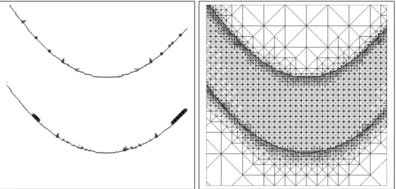
3.1.1 The adaptive concept

For resolving the interface which separates the fluid and the porous material we adapt the adaptive concept provided in [28, 29] to the present situation. We base the concept only upon the gradient flow structure, thus the Cahn–Hilliard equation, and derive a posteriori error estimates up to higher order terms for the approximation of∇ϕand ∇w.

We define the following errors and residuals:

eϕ=ϕ_h−ϕ, ew =w_h−w, r⁽_h¹⁾=ϕ_h−ϕ^k, r⁽_h²⁾=α^′_ε(ϕ_h) (1

2∣u_h∣²−u_h⋅q_h) +λ_s(ϕ_h) −γ

εϕ^k−w_h, η⁽_T¹⁾

E = ∑

E⊂T

h¹_E^/2∥[∇w_h]_E∥_L²_(E), η⁽_T²⁾

E = ∑

E⊂T

h¹_E^/2∥[∇ϕ_h]_E∥_L²_(E), η⁽_N¹⁾=h²_N∥r_h⁽¹⁾−R⁽_N¹⁾∥²_L²_(ωN), η⁽_N²⁾=h²_N∥r⁽_h²⁾−R⁽_N²⁾∥²_L²_(ωN). The values η⁽_Nⁱ⁾, i=1,2 are node-wise error values, while η_T⁽ⁱ⁾

E, i= 1,2 are edgewise error contributions, where for each triangleT the contributions over all edges ofT are summed up. For a node N ∈ N^k+1 we by ω_N denote the support of the piecewise linear basis function located atN and set h_N ∶=diam(ω_N). The value R_N⁽ⁱ⁾∈R, i=1,2 can be chosen arbitrarily. Later they represent appropriate means. By [⋅]E we denote the jump across the face E in normal direction νE pointing from simplex with smaller global number to simplex with larger global number. ν_E denotes the outer normal at Ω of E⊂∂Ω.

To obtain a residual based error estimator we follow the construction in [29, Sec. 7.1].

We further use [12, Cor. 3.1] to obtain lower bounds for the terms η_N⁽¹⁾ and η_N⁽²⁾. For convenience of the reader we state [12, Cor. 3.1] here.

Theorem 4 ([12, Cor. 3.1]). There exists a constant C >0 depending on the domain Ω and on the regularity of the triangulation T such that

∫_ΩR(u− Iu)dx+ ∫_EJ(u− Iu)ds

≤C∥∇u∥L^p(Ω)( ∑

N∈N

h^q_N∥R−RN∥^q_Lp(ωN)+ ∑

T∈T

hT∥J∥^q_Lq(E∩∂T))

1/q

holds for all J ∈L^q(E), R∈L^q(Ω), u∈W^1,p(Ω), and arbitraryR_N ∈R for N ∈ N, where 1<p, q< ∞ satisfy ¹_p+¹_q =1.

Here I ∶ L¹(Ω) → V^T denotes a modification of the Cl´ement interpolation operator proposed in [12, 13]. In [13] it is shown, that in general the error contributions arising from the jumps of the gradient of the discrete objects dominate the error contributions arising from triangle wise residuals. In our situation it is therefore sufficient to use the error indicators η_T⁽ⁱ⁾

E, i = 1,2, in an adaptation scheme to obtain well resolved meshes.

let us assume that R ∈ H¹(Ω) in Corollary 4. Then with RN = ∫ωNRdx we obtain

∥R−R_N∥L²(Ω)≤C(ω_N)∥∇R∥_L²_(Ω), andC(ω_N) ≤diam(ω_N)π⁻¹, cf. [36].

Since the construction of the estimator is standard we here only briefly describe the procedure. We use the errorsew andeϕ as test functions in (21a) and (21b), respectively.

Sincee_w, e_ϕ∈H¹(Ω)they are valid test functions in (17). Subtracting (21a) and the weak form of (17a), tested by ew, as well as subtracting (21b) and the weak form of (17b), tested byeϕ and adding the resulting equations yields

τ∥∇ew∥²_L²_(Ω)+γε∥∇eϕ∥²_L²_(Ω)

+ (λs(ϕh) −λs(ϕ), eϕ)_L2(Ω)+ ([α^′_ε(ϕh) −α^′_ε(ϕ)] (1

2∣uh∣²−uh⋅q_h), eϕ)

L²(Ω)

≤F⁽¹⁾((ϕ_h, w_h), e_w) +F⁽²⁾((ϕ_h, w_h), e_ϕ) + (α^′_ε(ϕ) [(1

2∣u∣²−u⋅q) − (1

2∣u_h∣²−u_h⋅q_h)], eϕ)

L²(Ω).

For convenience we investigate the term F⁽¹⁾((ϕ_h, w_h), ew). Since Iew∈ V¹(T^k+1) it is a valid test function for (21a). We obtain

F⁽¹⁾((ϕ_h, w_h), ew) =F⁽¹⁾((ϕ_h, w_h), ew− Iew)

=τ⁻¹∫_Ω(ϕ_h−ϕ^k)(e_w− Ie_w)dx+ ∫_Ω∇w_h⋅ ∇(e_w− Ie_w)dx +τ⁻¹∫_Ωr_h⁽¹⁾(e_w− Ie_w)dx+ ∑

E⊂E∫_E[∇w_h]_E(e_w− Ie_w)ds.

Applying Corollary 4 now gives F⁽¹⁾((ϕ_h, w_h), e_w)

≤C∥∇ew∥_L²_(Ω)(τ⁻² ∑

N∈N

h²_N∥r⁽_h¹⁾∥²_L²_(ωN)+ ∑

T∈T

hT∥ [∇w_h]_E∥²_L²_(∂T))

1/2

.

For F⁽²⁾((ϕ_h, w_h), e_ϕ) a similar result holds. Using Young’s inequality we obtain the following theorem.

Theorem 5. There exists a constant C >0 independent of τ, γ, ε, s and h ∶=maxT∈T hT

such that there holds:

τ∥∇ew∥²_L²_(Ω)+γε∥∇eϕ∥²

+ (λs(ϕ_h) −λs(ϕ), eϕ)_L²_(Ω)+ ([α^′_ε(ϕ_h) −α^′_ε(ϕ)] (1

2∣u_h∣²−u_h⋅q_h), eϕ)

L²(Ω)

≤C(η_Ω² +η²_h.o.t.), where

η²_Ω∶= 1

τ ∑

N∈N^k+1

(η_N⁽¹⁾)²+ 1 γε ∑

N∈N^k+1

(η⁽_N²⁾)²+τ ∑

T∈T^k+1

(η⁽_E¹⁾)²+γε ∑

T∈T^k+1

(η_E⁽²⁾)², and

η²_h.o.t.∶= 1 γε∑

T

∥α^′_ε(ϕ) ((1

2∣uh∣²−uh⋅q_h) − (1

2∣u∣²−u⋅q))∥²

L²(T). Remark 7. 1. Sinceλ_s is monotone there holds(λ_s(ϕ_h) −λ_s(ϕ), e_ϕ)_L²_(Ω)≥0.

2. We note that due to Assumption(A6)and the convexity ofα_εwe obtain([α^′_ε(ϕ_h) −α^′_ε(ϕ)] (¹₂∣u_h∣²−u_h⋅q_h), e_ϕ)_L2(Ω)≥ 0.

3. Due to using quadratic elements for both the velocity fieldu_hand the adjoint velocity field q_h we expect that the termη_h.o.t. can be further estimated with higher powers of h. It therefore is neglected in our numerical implementation.

4. The values R⁽_Nⁱ⁾, i = 1,2 can be chosen arbitrarily in R. By using the mean value R⁽_Nⁱ⁾= ∫^ωNr_h⁽ⁱ⁾dx and the Poincar´e-Friedrichs inequality together with estimates on the value of its constant ([36]) the terms η⁽_Nⁱ⁾, i=1,2 are expected to be of higher order and thus are also are neglected in the numerics.

5. Efficiency of the estimator up to terms of higher order can be shown along the lines of [29, Sec. 7.2] by the standard bubble technique, see e.g. [1].

For the adaptation process we use the error indicators η⁽_T¹⁾

E and η⁽_T²⁾

E in the following D¨orfler marking strategy ([15]) as in [28, 29].

The adaptive cycle We define the simplex-wise error indicatorηTE as η_TE =η_T⁽¹⁾

E +η⁽_T²⁾

E, and the set of admissible simplices

A = {T ∈ T^k+1∣amin≤ ∣T∣ ≤amax},

whereamin and amax are the a priori chosen minimal and maximal sizes of simplices. For adapting the computational mesh we use the following marking strategy:

1. Fix constantsθ^r andθ^cin(0,1).

2. Find a setM^E ⊂ T^k+1 such that

∑

T∈M^E

η_TE ≥θ^r ∑

T∈T^k+1

η_TE.

3. Mark eachT ∈ (M^E∩ A) for refinement.

4. Find the setC^E⊂ T^k+1 such that for each T ∈ C^E there holds ηTE ≤ θ^c

N_T ∑

T∈T^k+1

ηTE.

5. Mark allT ∈ (C^E∩ A)for coarsening.

HereN_T denotes the number of elements ofT^k+1.

We note that by this procedure a simplex can both be marked for refinement and coarsening. In this case it is refined only. We further note, that we apply this cycle once per time step and then proceed to the next time instance.

4 Numerical examples

In this section we discuss how to choose the values incorporated by our porous material – diffuse interface approach.

We note that there are a several approaches on topology optimization in Navier–Stokes flow, see e.g. [6, 26, 32, 35, 37]. On the other hand it seems, that so far no quantitative values to describe the optimal shapes are available in the literature. All publications we are aware of give qualitative results or quantitative results that seem not to be normalized for comparison with other codes.

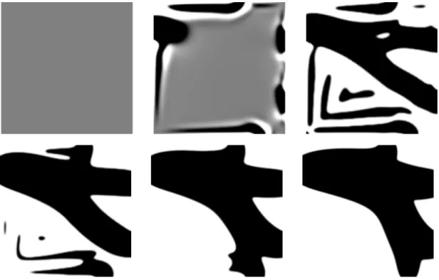
In the following we start with fixing the interpolation functionαεand the parameters τ,s, andε. We thereafter in Section 4.4 investigate how the phase field approach can find optimal topologies starting from a homogeneously distributed porous material.

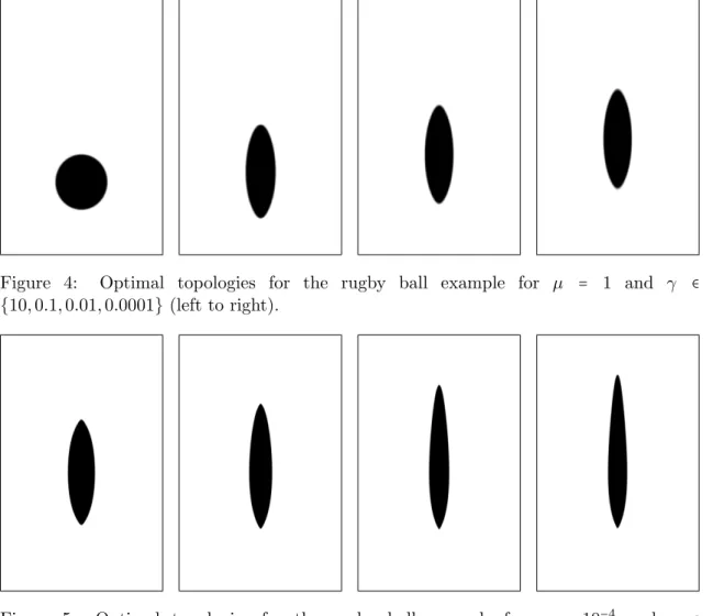
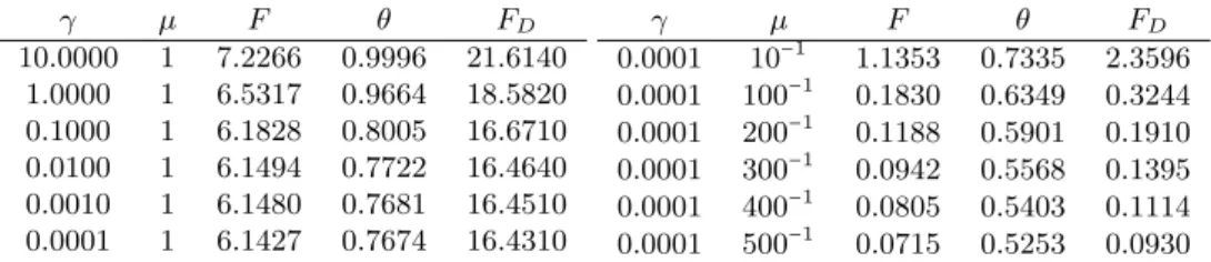
In Section 4.5 we present numerical experiments for the rugby ball, see als [6], [37] and [39]. Here we provide comparison value for the friction drag of the optimized shape, and as second comparison value we introduce the circularity describing the deviation of the ball from a circle.

As last example, and as outlook, we address the optimal shape of the embouchure of a bassoon in Section 4.6.

In the following numerical examples we always assume the absence of external forces, hencef ≡0. The optimization aim is always given by minimizing the dissipative energy (2), which in the absence of external forces is given by

F = ∫_Ωµ

2∣∇u∣²dx.

The Moreau–Yosida parameter in all our computations is set to s=10⁶. We do not investigate its couplings to the other parameters involved.

For later referencing we here state the parabolic in-/outlet boundary data that we use frequently throughout this section

g(x) =⎧⎪⎪⎪

⎨⎪⎪⎪⎩

h(1− (^x_l⁻_/^m₂ )²) if∣x−m∣ <l/2,

0 otherwise.

(22) In the following this function denotes the normal component of the boundary data at por- tions of the boundary, where inhomogeneous Dirichlet boundary conditions are prescribed.

The tangential component is set to zero if not mentioned differently.

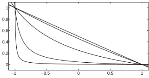
−1 −0.5 0 0.5 1 0

0.2 0.4 0.6 0.8 1

Figure 1: The shape of the interpolation function α_ε for q =10ⁱ, i= −2, . . .2 (bottom to top).

4.1 Time step adaptation

For a faster convergence towards optimal topologies we adapt the length of the time steps τ^k+1. Here we use a CFL-like condition to ensure that the interface is not moving too fast into the direction of the flux∇w_h. With

τ^∗= min

T∈T^k

hT

∥∇w^k∥L^∞(T)

we set

τ^k+1=max(τmax, τ^∗),

whereτmaxdenotes an upper bound on the allowed step size and typically is set toτmax= 10⁴. Thus the time step size for the current step is calculated using the variable w^k from the previous time instance. We note that especially for ∇w^k→0 we obtaintk → ∞, and thus when we approach the final state, we can use arbitrarily large time steps. We further note, that if we choose a constant time step the convergence towards a stationary point of the gradient flow in all our examples is very slow and that indeed large time steps close to the equilibrium are required.

4.2 The interfacial width

As discussed in Section 2 the phase field problem can be verified to approximate the sharp interface shape optimization problem asε↘0 in a certain sense. Hence we assume that the phase field problems yield reasonable approximations of the solution for fixed but smallε>0, and we do not vary its value. Typically, in the following we use the fixed value ε=0.005.

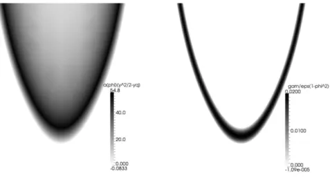
4.3 The interpolation function

We set (see [6])

αε(ϕ) ∶= α 2√

ε(1−ϕ) q

(ϕ+1+q), (23)

with α > 0 and q > 0. In our numerics we set α = 50. In Figure 1 the function α_ε is depicted in dependence of q. We have αε(−1) = αε = αε^−1/2 and Assumption (A4) is fulfilled, except that limε↘0αε(0) < ∞ holds. Anyhow, the numerical results with this choice of α_ε are reasonable and we expect that this limit condition has to be posed for technical reasons only. To fulfill Assumption (A5) we cut αε at ϕ≡ϕc>1 and use any smooth continuation yieldingαε(ϕ) ≡const forϕ≥ϕc.