Sharp interface limit for a phase field model in structural optimization

Universit¨ at Regensburg Mathematik

Sharp interface limit for a phase field model in structural optimization

Luise Blank, Harald Garcke, Claudia Hecht and Christoph Rupprecht

Preprint Nr. 17/2014

STRUCTURAL OPTIMIZATION

LUISE BLANK^∗, HARALD GARCKE^∗, CLAUDIA HECHT^∗, ^AND CHRISTOPH RUPPRECHT^∗

Abstract. We formulate a general shape and topology optimization problem in structural optimization by using a phase field approach. This problem is considered in view of well-posedness and we derive optimality conditions. We relate the diffuse interface problem to a perimeter penalized sharp interface shape optimization problem in the sense of Γ-convergence of the reduced objective functional. Additionally, convergence of the equations of the first variation can be shown. The limit equations can also be derived directly from the problem in the sharp interface setting. Numerical computations demonstrate that the approach can be applied for complex structural optimization problems.

Key words. Shape and topology optimization, linear elasticity, sensitivity analysis, optimality conditions, Γ-convergence, phase field method, diffuse interface, numerical simulations.

AMS subject classification. 35Q74, 35R35, 49Q10, 49Q12, 74B05, 74Pxx.

1. Introduction. In structural optimization one tries to find an optimal ma- terial configuration of two different elastic materials in some fixed container, where optimal means that a certain objective functional depending on the behaviour of the elastic materials is minimized. The control here is represented by the material distri- bution. Applications of shape and topology optimization reach from crashworthiness of transport vehicles and tunnel design to biomechanical applications such as bone remodelling. Structural optimization has turned out to be helpful in solving automa- tive design problems in order to maximize the stiffness of vehicles for instance or to reduce the stresses to improve durability, see for instance [8].

One of the first approaches of finding the optimal material distribution in presence of two materials can be found in [37]. However the problem of finding optimal structures in mechanical engineering dates at least back to the beginning of the 20th century when Michell [32] considered optimal truss layouts. It has turned out, that generally those problems are not well-posed, because oscillations occur on a very fine scale, see for example [9], and hence several ideas have been developed to overcome this issue.

One important contribution is certainly the idea of using a perimeter penalization in optimal shape design and considering this problem in the framework of Caccioppoli sets, see [5], in order to prevent the above-mentioned oscillations. Additionally, it turns out that it is difficult to control the state variables if they are only given on varying domains of definitions. And so a so-called ersatz material approach has been introduced, see for instance [2, 16]. Here, one replaces the void regions by a fictitious material which may have a very low stiffness. We also remark that there appear many problems of practical relevance where one wants to fill a given domain with two different materials (and not one material and void) such that after an applied load an objective functional is minimized. Having this in mind it is the main goal of this paper to analyze and numerically solve problems with two materials, whether fictious or not.

We start by stating a perimeter penalized shape optimization problem with a general

∗Fakult¨at f¨ur Mathematik, Universit¨at Regensburg, 93040 Regensburg, Germany ({Luise.Blank, Harald.Garcke, Claudia.Hecht, Christoph.Rupprecht}@mathematik.uni-regensburg.de).

1

objective functional in Section 2.2. This is in a simplified form given as

(ϕ,minu)J0(ϕ,u) ∶= ∫_ΩhΩ(x,u)dx+ ∫_Γ

g

hΓ(s,u)ds+γc0PΩ({ϕ=1}) subject to ∫_ΩC(ϕ) (E (u) − E (ϕ)) ∶ E(v)dx= ∫_Ωf⋅vdx+∫_Γ

g

g⋅vds ∀v.

(1)

After showing well-posedness we derive necessary optimality conditions by geometric variations without any additional regularity assumption on the minimizing set other than being a Caccioppoli set. This seems to be new as classical shape derivatives always assume at least an open Lipschitz domain as minimizer, see [1, 3, 4, 31], and they do not treat a general objective functional. We also show that the obtained conditions are consistent with existing results obtained with shape derivatives if the minimizing shape inherits a certain regularity.

Then we approximate this problem by using a phase field approach where the free boundary is replaced by a diffuse interface with small thickness related to a parameter ε>0. Hence, as in [16], the perimeter functional is replaced by the Ginzburg-Landau energy and the optimization problem (1) reads as

(ϕ,minu)Jε(ϕ,u)∶= ∫_ΩhΩ(x,u)dx+∫_Γ

g

hΓ(s,u)ds+γ∫_Ωε

2∣∇ϕ∣²+1

εψ(ϕ)dx subject to ∫_ΩC(ϕ) (E(u) −E(ϕ)) ∶E(v)dx= ∫_Ωf⋅vdx+∫_Γ

g

g⋅vds ∀v.

(2)

After discussing well-posedness and necessary optimality conditions for the phase field problem we consider the sharp interface limit. To be precise, we show Γ- convergence of the reduced objective functional as the interfacial width, i.e. ε, tends to zero. Moreover, we show that the equations of the optimality systems converge.

We hereby generalize findings from literature where this result has already been indi- cated in [11] by formal asymptotics for certain objective functionals.

The paper is structured as follows: In Section 2 we introduce the exact problem for- mulations, discuss well-posedness, optimality conditions and the sharp interface limit.

The derivation of the optimality conditions can be found in Section 4 and some proofs of the sharp interface convergence results are collected in Section 5. The numerical approach and results are given in Section 3.

2. Discussion of the problems and convergence results.

2.1. Notation and assumptions. Before formulating the shape optimization problems we give a brief introduction into the most important quantities and equations in linearized elasticity and fix some notation. We refer the reader to [17, 18, 24] and references therein for details. We first assume to have in the holdall container Ω two open subsets Ω1 and Ω2 which are separated by a hypersurface Γ=∂Ω1∩∂Ω2. The two subsets should correspond to two different elastic materials whose displacement fields are described by one variable u∶Ω→R

d. To be precise, u∣^Ωi corresponds to the displacement field of thei-th material wherei∈{1,2}. We divide the boundary of Ω into two parts, one Dirichlet part where we can prescribe the displacement field, and a Neumann part where the applied boundary forces are acting.

(A1) Ω⊂^Rdis a bounded Lipschitz domain with outer unit normalnandd∈{2,3}. Moreover, assume∂Ω=ΓD∪Γg withH^d−1(ΓD)>0 and ΓD∩Γg=∅. We remark that we denote ^Rd-valued functions and spaces consisting of ^Rd-valued functions in boldface.

For elastic materials the following equilibrium constraints hold in Ωi,i∈{1,2}:

−∇ ⋅ (D2W_i(x,E(u)))=f in Ωi, (3a) D2Wi(x,E(u)) ⋅n=g on Γg∩∂Ωi, (3b) u=u_D on ΓD∩∂Ωi, (3c) where:

(A2) g ∈L²(Γg) is the given applied surface load, f ∈ L²(Ω) the given applied surface load and for simplicity we assume for the following considerations uD≡0.

On the interface Γ∶=∂Ω1∩∂Ω2 the boundary conditions are given by certain trans- mission properties, which follow from (5). Moreover, E(u) ∶= ¹2(∇u+ ∇u^T) is the so-called linearized strain, whereon the linear theory is based andW_i∶Ω×^Rd×d→R

denotes the elastic free energy density of the i-th material. We use W_i(x,E) ∶=

1

2(E−Ei) ∶Ci(E−Ei)forE ∈^Rd×d, which is in our case independent ofx∈^Rd. Here, Cⁱ∶^Rd×d→R

d×dis the elasticity tensor reflecting the material properties for material i=1 and i=2, respectively. Further, Ei ∈^Rd×d is the eigenstrain which is given as the value of the strain when thei-th material is unstressed. By D2W_i we denote the derivative with respect to the second component.

As already mentioned above, we have two different elastic materials inside the domain Ω. The design variable is a measurable function ϕ ∶ Ω → R, where {x ∈ Ω ∣ ϕ(x) = 1} = Ω1 describes the region where the first material is present up to a set of measure zero, and {x∈Ω∣ϕ(x)=−1} = Ω2 the region which is filled with the second material. In the sharp interface setting, ϕwill only take values in {±1} and thus Ω = Ω1∪Ω2∪Γ with Γ = ∂Ω1∩∂Ω2 being the separating hypersurface.

In contrast, the phase field approximation uses a design functionϕ having values in [−1,1]. Then, Ω=Ω1∪Ω2∪I whereI={−1<ϕ<1}is the diffuse interface of small thickness approximating the hypersurface Γ. Using ϕto describe the sharp as well as the diffuse interface model we describe the elasticity tensor and the eigenstrain as functions of the design variable ϕwhich interpolate between two different values for the two different materials. We introduce the following assumptions on the elasticity tensorC and we use the following assumptions:

(A3) LetC(ϕ)=(C^ijkl(ϕ))^di,j,k,l=1 be such that C^ijkl ∈C^1,1([−1,1]) fulfills point- wise the following symmetry propertiesCijkl(ϕ)= Cjikl(ϕ)= Cklij(ϕ)for all ϕ∈ [−1,1], i, j, k, l ∈ {1, . . . , d}. Moreover, we assume that there exist con- stantsC_C, c_C>0 such that

∣C(ϕ)A∶B∣≤CC∣A∣ ∣B∣, C(ϕ)A∶A≥cC∣A∣² (4) holds for all symmetric matricesA, B∈^Rd×dandϕ∈[−1,1].

(A4) Let the eigenstrain E ∈ C^1,1([−1,1],^Rd×d) be a function with symmetric values, i.e. E(ϕ)^T = E(ϕ)for allϕ∈[−1,1].

Remark 1.

1. The estimates (4) imply that the elasticity tensor interpolates between two finite positive definite tensors, thus in particular no “void”, i.e. regions without ma- terial, are allowed in this formulation. Anyhow, the possibility of modelling “void” is given by using the so-called ersatz material approach, where a very soft material ap- proximates the non-presence of material, cf. [11, 16]. Moreover, the elasticity tensor

is not depending on the phase field variableε>0introduced later on. Hence, an ersatz material approach depending on the phase field parameter ε>0 as it is employed in [11] cannot be used in this setting.

2. Following Vegard’s law, a commonly used assumption is that the eigenstrain interpolates linearly between the two values corresponding to the two materials. Then, Assumption(A4)is fulfilled.

Using these assumptions, a weak formulation of the state equations on the whole of Ω can be derived, if the design variable isϕ∈L¹(Ω)with∣ϕ∣≤1 a.e. in Ω:

Findu∈H¹_D(Ω)∶={u∈H¹(Ω) ∣u∣^ΓD =0}such that

∫ΩC(ϕ) (E(u)−E(ϕ))∶E(v)dx= ∫_Ωf⋅vdx+∫Γ_gg⋅vds ∀v∈H¹_D(Ω). (5) In any subregion{ϕ=±1}this yields exactly the weak formulation of (3). The state equation is in both the phase field and the sharp interface formulation given by (5), cf. Sections 2.2 and 2.3. Hence we directly state here the solvability result concerning this equation:

Lemma 2. For every ϕ ∈ L¹(Ω) with ∣ϕ∣ ≤ 1 a.e. in Ω there exists a unique u∈H¹_D(Ω)such that (5)is fulfilled. Moreover, the solutionu fulfills

∥u∥^H1(Ω)≤C(Ω,C,E) (∥f∥^L2(Ω)+∥g∥^L2(Γg)+1). (6) This defines a solution operatorS∶{ϕ∈L¹(Ω) ∣ ∣ϕ∣≤1 a.e. inΩ}→H¹_D(Ω). Idea of the proof. By making use of Korn’s inequality, this result is a direct conse- quence of Lax-Milgram’s theorem, cf. [30, Lemma 24.1].

For our shape and topology optimization problem, the goal is to minimize H(u)∶= ∫_ΩhΩ(x,u)dx+∫_ΓghΓ(s,u)ds (7) wherehΩ, hΓ fulfill

(A5) hΩ∶Ω×^Rd→RandhΓ∶Γg×^Rd→Rare Carath´eodory functions, i.e.

1. hΩ(⋅,v) ∶ Ω → R and hΓ(⋅,v) ∶ Γg → R are measurable for each v∈^Rd, and

2. hΩ(x,⋅), hΓ(s,⋅)∶^Rd→Rare continuous for almost everyx∈Ω and s∈Γg, respectively.

Moreover, assume that there exist functions a1 ∈ L¹(Ω), a2 ∈ L¹(Γg) and b1∈L^∞(Ω),b2∈L^∞(Γg)such that it holds

∣hΩ(x,v)∣≤a1(x)+b1(x)∣v∣² ∀v∈^Rd, a.e. x∈Ω, (8) and

∣hΓ(s,v)∣≤a2(s)+b2(s)∣v∣² ∀v∈^Rd, a.e. s∈Γg. (9) Additionally, we assume that the set

{∫_ΩhΩ(x,S(ϕ)(x))dx+∫_Γ

g

hΓ(s,S(ϕ)(s))ds∣ϕ∈L¹(Ω),∣ϕ∣≤1 a.e. in Ω} is bounded from below.

Remark 3. Due to [36], the Nemytskii operators

L²(Ω)^d∋v↦hΩ(⋅,v)∈L¹(Ω), L²(Γg)^d∋v↦hΓ(⋅,v)∈L¹(Γg)

are well-defined if and only if (8) and (9) are fulfilled and in this case the operators are continuous.

Assumptions (A1)-(A5) are the basic assumptions for the following considera- tions. To derive also first order optimality conditions we have to impose at some points additionally the following differentiability assumption.

(A6) For every fixed v∈^Rd we have hΩ(⋅,v)∈W^1,1(Ω)andhΓ(⋅,v)∈W^1,1(Γg). Let the partial derivatives D2hΩ(x,⋅),D2hΓ(s,⋅)exist for almost everyx∈Ω and s∈Γg, respectively. Moreover there exist ˆa1 ∈L²(Ω), ˆa2 ∈L²(Γg)and ˆb1∈L^∞(Ω), ˆb2∈L^∞(Γg)such that

∣D2hΩ(x,v) ∣≤aˆ1(x)+ˆb1(x)∣v∣ ∀v∈^Rd, a.e. x∈Ω (10) and

∣D2hΓ(s,v) ∣≤ˆa2(s)+ˆb2(s)∣v∣ ∀v∈^Rd, a.e. s∈Γg. (11) Remark 4. Under the Assumption (A6)the operators

F ∶L²(Ω)∋u↦∫ΩhΩ(x,u(x))dx, G∶L²(Γg)∋u↦∫Γ_ghΓ(s,u(s))ds are continuously Fr´echet differentiable and that the directional derivatives are given byDF(u) (v)= ∫^ΩD2hΩ(x,u)vdx,DG(u) (v)= ∫^ΓgD2hΓ(s,u)vds.

In the next remark, we outline how we could replace Assumptions(A5)and(A6) by weaker assumptions. In order to simplify the estimates in the following analysis we prefer(A5)and(A6).

Remark 5. We could generalise the results to objective functionals satisfying

∣hΩ(x,v)∣≤a1(x)+b1(x) ∣v∣^p, ∀v∈^Rd, a.e. x∈Ω (12) for some functions a1∈L¹(Ω)andb1∈L^∞(Ω), instead of requiring (8). Here, p≥2 has to be chosen such that H¹(Ω)↪L^p(Ω)is a compact imbedding, hence2≤p< ∞ ford=2 and2≤p<6 ford=3. We then obtain that L^p(Ω)^d∋v↦hΩ(⋅,v)∈L¹(Ω) is well-defined and continuous and all proofs can be adapted. In this case, we have to replace (10) in Assumption (A6) by ∣D2hΩ(x,v) ∣ ≤ aˆ1(x)+ˆb1(x)∣v∣^p−1 for all v ∈ ^Rd and a.e. x∈ Ω where aˆ1 ∈ L^p/p−1(Ω), ˆb1 ∈ L^∞(Ω) to obtain that L^p(Ω) ∋ u↦∫^ΩhΩ(x,u(x))dxis continuously Fr´echet differentiable. The same holds for the choice of hΓ.

In order to obtain a well-posed problem we add to the cost functional Hin (7) a regularization term. In the sharp interface problem a multiple of the perimeter of the free boundary between the two materials is used. The exact definition of the perimeter is introduced now. Since we describe the sharp interface model by a design variableϕ∶Ω→{±1}, where{ϕ=±1}describe the two different materials, this design variable is going to be a function of bounded variation. We give here a brief intro- duction in the notation of Caccioppoli sets and functions of bounded variations, but for a detailed introduction we refer to [6, 25]. We call a functionϕ∈L¹(Ω)a function of bounded variation if its distributional derivative is a vector-valued finite Radon

measure. The space of functions of bounded variation in Ω is denoted by BV(Ω), and by BV(Ω,{±1}) we denote functions in BV(Ω) having only the values ±1 a.e.

in Ω. We then call a measurable setE⊂Ω Caccioppoli set ifχE∈BV(Ω). For any Caccioppoli setE, one can hence define the total variation∣DχE∣ (Ω)of DχE, as DχE

is a finite measure. This value is then called the perimeter ofE in Ω and is denoted byPΩ(E)∶=∣DχE∣ (Ω).

We include additionally a volume constraint in the optimization problem. By assuming that the design variable ϕ fulfills ∫^Ωϕdx ≤ β∣Ω∣, which is equivalent to

∣{ϕ=1}∣≤ ^(β+1)2 ∣Ω∣ and ∣{ϕ=−1}∣≥ ^(1−β)2 ∣Ω∣, for some fixed constant β∈(−1,1)we prescribe a maximal amount of the material corresponding to {ϕ= 1} (and thus a minimal amount of{ϕ=−1}) that can be used during the optimization process.

Our admissible design variables for the sharp interface problem hence are chosen in the set

Φ⁰_ad∶={ϕ∈BV (Ω,{±1}) ∣∫_Ωϕdx≤β∣Ω∣}. (13) In the phase field formulation of the shape optimization problem we approximate the perimeter by the Ginzburg-Landau energy

E_ε(ϕ)∶= ∫_Ωε

2∣∇ϕ∣²+1

εψ(ϕ)dx (14)

with a double obstacle potentialψ∶^R→R∶=^R∪{∞}given by ψ(ϕ)∶=⎧⎪⎪

⎨⎪⎪⎩

ψ0(ϕ), if ∣ϕ∣≤1

+∞, if ∣ϕ∣>1, ψ0(ϕ)∶= 1

2(1−ϕ²). (15) The functionals(E_ε)^ε>0Γ-converge inL¹(Ω)toϕ↦c0PΩ({ϕ=1})withc0∶= ∫⁻¹¹√

2ψ(s)ds=

π

2 asε↘0, see for instance [33, 34].

In the phase field setting, the design variableϕis allowed to have values in[−1,1] and thus there may be a transition area between the areas{ϕ=−1}and{ϕ=1}. The admissible set in the phase field setting is given by

Φad∶={ϕ∈H¹(Ω) ∣∫_Ωϕdx≤β∣Ω∣,∣ϕ∣≤1 a.e. in Ω} (16) and the extended admissible set by Φad∶={ϕ∈H¹(Ω) ∣ ∣ϕ∣≤1 a.e. in Ω}.

Remark 6. Instead of ∫^Ωϕdx≤ β∣Ω∣ we could also use an equality constraint of the form ∫^Ωϕdx= β∣Ω∣. This prescribes then the exact volume fraction of each material in advance. In this setting, the same analysis can be carried out. The results whereon our sharp interface analysis is based only deal with an equality constraint, see for instance [15, 26, 33].

As we derive first order optimality conditions by varying the free boundary be- tween the two materials with transformations, we introduce here the admissible trans- formations and its corresponding velocity fields:

Definition 7 (V^ad, T^ad). The spaceV^ad of admissible velocity fields is defined as the set of all V ∈C([−τ, τ]×Ω,^Rd), where τ > 0 is some fixed, small constant, such that it holds:

(V1) (V1a) V(t,⋅)∈C²(Ω,^Rd),

(V1b) ∃C>0: ∥V(⋅, y)−V(⋅, x)∥C([−τ,τ],^Rd)≤C∣x−y∣ ∀x, y∈Ω, (V2) V(t, x)⋅n(x)=0 for allx∈∂Ω,

(V3) V(t, x)=0for everyx∈ΓD.

Then the spaceTadof admissible transformations is defined as solutions of the ordinary differential equation

∂tTt(x)=V(t, Tt(x)), T0(x)=x (17) withV ∈ Vad, which gives some T∶(−τ ,˜ τ˜)×Ω→Ω, with0<τ˜ small enough.

We often use the notation V(t)=V(t,⋅).

Remark 8. Let V ∈ V^ad and T ∈ V^ad be the transformation associated toV by (17). ThenTt∶Ω→Ωis bijective and T(⋅, x)∈C¹((−τ, τ),^Rd)for all x∈Ωandτ>0 small enough. These and other properties are discussed in detail in [20, 22].

We finish this introduction by two typical examples which are commonly used as objective functionals in structural optimization. For a deeper discussion on those problems and some further applications we refer for instance to [8].

Example 9 (Mean compliance). One commonly used objective in structural optimization is the minimization of the mean compliance, which is for a structure in its equilibrium configuration given by∫^Ωf⋅udx+∫^Γgg⋅uds. The aim of minimizing this objective functional can be interpreted as maximizing the stiffness under the given forces or as minimizing the stored mechanical energy. We notice, that this is equivalent to minimizing ∫^ΩC(ϕ) (E(u)−E(ϕ))∶E(u)dxifu solves the state equations(5).

Example 10 (Compliant mechanism). The typical compliant mechanism objec- tive functional used in topology optimization is given by the tracking type functional

1

2∫^Ωc∣u−uΩ∣²dx where uΩ∈ L²(Ω) is some desired displacement, andc ∈L^∞(Ω), c≥0, is a weighting factor.

In the following, by minimizers we always mean global minimizers.

2.2. Perimeter penalized shape optimization problem. The sharp inter- face problem that we consider in this section is given by

(ϕ,minu)J0(ϕ,u)∶=H(u)+γc0PΩ({ϕ=1})=

= ∫_ΩhΩ(x,u)dx+∫_Γ

g

hΓ(s,u)ds+γc0PΩ({ϕ=1}) (18) with(ϕ,u)∈Φ⁰_ad×H¹_D(Ω)such that (5) holds, i.e.

∫_ΩC(ϕ) (E(u)−E(ϕ))∶E(v)dx= ∫_Ωf⋅vdx+∫_Γ

g

g⋅vds ∀v∈H¹_D(Ω). (19) This is a topology and shape optimization problem, where ϕ ∈ Φ⁰_ad = {ϕ ∈ BV(Ω,{±1}) ∣∫^Ωϕdx≤β∣Ω∣}plays the role of the design variable, and can only have the discrete values±1. The perimeter in the cost functional ensures the existence of a minimizer where the weighting factorγ>0 can be arbitrary. In the remainder of this subsection we summarize often results where the proofs are given later in this paper or in some previous work. Studying the reduced objective functionalj0∶L¹(Ω)→R,

j0(ϕ)∶=⎧⎪⎪

⎨⎪⎪⎩

J0(ϕ,S(ϕ)), ifϕ∈Φ⁰_ad,

+∞, otherwise,

we obtain by using the direct method in the calculus of variations the well-posedness of the optimization problem:

Theorem 11. Under the assumptions(A1)-(A5), there exists at least one min- imizer of (18)−(19).

Proof. We use that (18)−(19) is equivalent to minϕ∈L¹(Ω)j0(ϕ). According to Assumption(A5), the objective functional j0 is bounded from below and hence we may choose a minimizing sequence(ϕ_k)^k∈N forj0. ThusPΩ({ϕ_k=1})=∣Dϕk∣(Ω)is uniformly bounded. We obtain therefrom and the fact that∥ϕ_k∥L^∞(Ω)≤1 for allk∈^N that (ϕk)^k∈N is uniformly bounded in BV(Ω). As BV(Ω) imbeds compactly into L¹(Ω), we hence find that(ϕk)^k∈N has a subsequence (ϕkl)^l∈N converging in L¹(Ω) and pointwise to some limit element ϕ∈ BV(Ω). From the pointwise convergence we obtain ϕ(x)∈ {±1} for almost every x∈Ω and the convergence in L¹(Ω)yields directly ∫^Ωϕdx≤β∣Ω∣. Hence we haveϕ∈Φ⁰_ad. From Lemma 24, which is given in Section 5, we obtain thatϕ↦∫^ΩhΩ(x,S(ϕ))dx+∫^ΓghΓ(s,S(ϕ))dsis continuous in L¹(Ω). Moreover, the perimeter functionalϕ↦PΩ({ϕ=1})is lower semicontinuous in L¹(Ω), see [6], and thus we obtainj0(ϕ)≤lim infl→∞j0(ϕ_kl). This shows that ϕ is a minimizer ofj0, and hence(ϕ,S(ϕ))is a minimizer of (18)−(19).

Our next aim is to deduce first order necessary optimality conditions. For this purpose, we use the ideas of shape calculus, which means we apply geometric vari- ations. As already mentioned in the introduction we do not impose any additional regularity assumption on the minimizing set. We obtain:

Theorem 12. Assume (A1)-(A6). Then for any minimizer (ϕ0,u0)∈ Φ⁰_ad× H¹_D(Ω)of(18)−(19)the following necessary optimality conditions hold: There exists a Lagrange multiplierλ0≥0 for the integral constraint such that

∂_t∣^t=0j0(ϕ0○T_t⁻¹)=−λ0∫_Ωϕ0divV(0)dx, λ0(∫_Ωϕ0dx−β∣Ω∣)=0 (20)

holds for allT ∈ T^adwith corresponding velocityV ∈ V^ad, where the derivative is given by the following formula:

∂_t∣^t=0j0(ϕ0○T_t⁻¹)=∂_t∣^t=0H(S(ϕ0○T_t⁻¹))+γc0∫_Ω(divV(0)−ν⋅ ∇V(0)ν)d∣DχE0∣ (21) and

∂t∣^t=0H(S(ϕ0○T_t⁻¹))= ∫_Ω[DhΩ(x,u0) (V(0),u˙0[V])+hΩ(x,u0)divV(0)]dx+ +∫_Γ

g

[DhΓ(s,u0) (V(0),u˙0[V])+hΓ(s,u0) (divV(0)−n⋅ ∇V(0)n)]ds

(22)

withν∶= ∣D^Dχχ^E0E0∣being the generalised unit normal on the Caccioppoli setE0∶={ϕ0=1},

compare [6]. Moreover, u˙0[V]∈H¹_D(Ω)is given as the solution of

∫_ΩC(ϕ0)E(u˙0[V])∶E(v)dx= ∫_ΩC(ϕ0)1

2(∇V(0)∇u0+(∇V(0)∇u0)^T)∶E(v)+

+C(ϕ0) (E(u0)−E(ϕ0))∶1

2(∇V(0)∇v+(∇V(0)∇v)^T)−

−C(ϕ0) (E(u0)−E(ϕ0))∶E(v)divV(0)dx−∫_Ωf⋅DvV(0)dx−∫_Γgg⋅DvV(0)ds (23) which has to hold for allv∈H¹_D(Ω).

The proof of this theorem can be found in Section 4.

Remark 13. If we assume thatΓg has C²-regularity, (22)can be rewritten into a more convenient form by using the identity divΓ_gV(0)= divV(0)−n⋅ ∇V(0)non Γg.

We can now reformulate those optimality conditions under more regularity as- sumptions on the minimizing setE0={ϕ0=1}and the given data. In particular, we can then compare our results to those obtained in literature, see Remark 15.

Theorem 14. Assume (A1)-(A6). Let (ϕ0,u0)∈Φ⁰_E×H¹_D(Ω) be minimizers of(18)−(19). Assume there are open setsΩ1,Ω2⊂Ωsuch thatϕ0=1a.e. onΩ1 and ϕ0=−1 a.e. in Ω2. Let g ∈H¹²(∂Ω)and the objective functional is assumed to be chosen in such a way that D2hΩ(⋅,u)∈L²(Ω)and D2hΓ(⋅,u)∈H¹²(Γg) for all u∈ H¹(Ω). IfhΓ(⋅,u0(⋅)) /≡0, we assume additionally thatΓghasC²-regularity. Assume that Γ0∶=∂Ω1∩∂Ω2∈C² and d(Γ0, ∂Ω)>0. By[w]^Γ0(x)∶=w∣^Ω1(x)−w∣^Ω2(x) we denote the jump ofw along the interfaceΓ0, and ν is the outer unit normal onΩ1. Let κ= divΓ0ν be the mean curvature ofΓ0. Then the optimality conditions derived in Theorem 12 are equivalent to the following system:

γc0κ−[C(ϕ0) (E(u0)−E(ϕ0))∶E(q0)]Γ0+ +[C(ϕ0) (E(u0)−E(ϕ0))ν⋅∂_νq0]Γ0+

+[C(ϕ0)E(q0)ν⋅∂νu0]^Γ0+2λ0+[hΩ(x,u0)]^Γ0=0 onΓ0

⎫⎪⎪⎪⎪

⎪⎬⎪⎪⎪⎪⎪

⎭

(24)

λ0(∫Ωϕ0dx−β∣Ω∣)=0, λ0≥0, ∫Ωϕ0dx≤β∣Ω∣, (25) together with the state equation (5)connecting ϕ0 andu0. Here, the adjoint variable q0∈H¹_D(Ω)is the unique solution of the adjoint equation

∫_ΩC(ϕ0)E(q0)∶E(v)dx= ∫_ΩD2hΩ(x,u0)vdx+∫_Γ

g

D2hΓ(s,u0)vds ∀v∈H¹_D(Ω). (26) The statement of Theorem 14 can be shown by using basic calclations such as integration by parts and chain rule. This calculation has been carried out for instance in [30, Theorem 25.3].

Remark 15. In [11] the same optimality system for the sharp interface set- ting has been derived from the phase field model by formally matched asymptotics for the mean compliance and compliant mechanism problems mentioned in Examples 9 and 10. However, no eigenstrain has been taken into account in [11] while this is included in the above problem setting. Applying shape sensitivity analysis yields the same result as we have found in Theorem 14 (see e.g. [1, 4, 31]).

2.3. Phase field approximation. In a diffuse interface setting in terms of a phase field formulation the shape and topology optimization problem of finding the optimal material distribution of two given materials is given by

(ϕ,minu)Jε(ϕ,u)∶=H(u)+γEε(ϕ)=

= ∫_ΩhΩ(x,u)dx+∫_Γ

g

hΓ(s,u)ds+γ∫_Ωε

2∣∇ϕ∣²+1

εψ(ϕ)dx (27) with(ϕ,u)∈Φad×H¹_D(Ω)such that (5) holds, i.e.

∫_ΩC(ϕ) (E(u)−E(ϕ))∶E(v)dx= ∫_Ωf⋅vdx+∫_Γ

g

g⋅vds ∀v∈H¹_D(Ω). (28) Hence the design variable in this problem is given byϕ∈Φad={ϕ∈H¹(Ω) ∣∫^Ωϕdx≤ β∣Ω∣,∣ϕ∣≤1 a.e. in Ω}. The regions filled with material one or two are represented by {x∈Ω∣ϕ(x)=1}and {x∈Ω∣ϕ(x)=−1}, respectively. The design variable ϕis also allowed to take values between minus one and one, which leads to a small transitional area whose thickness is proportional to a small parameterε>0. Thus, asεtends to zero, we will arrive in a sharp interface problem and the interfacial layer vanishes.

As was already discussed in Section 2.1, the Ginzburg-Landau energy E_ε, compare (14), appearing in the objective functional is essential for the existence of a minimizer and(E_ε)εΓ-converge to a multiple of the perimeter functional asεtends to zero, cf.

[33, 34]. The parameterγ>0 is an arbitrary fixed constant and can be considered as a weighting factor of the perimeter penalization.

We know from Lemma 2 that there is a solution operatorS for the constraints (28). Thus, we can reformulate the optimization problem into min_ϕ∈L¹₍Ω)jε(ϕ)where j_ε∶L¹(Ω)→R,

jε(ϕ)∶=⎧⎪⎪

⎨⎪⎪⎩

J_ε(ϕ,S(ϕ)), ifϕ∈Φad,

+∞, otherwise,

is the reduced objective functional. We start by discussing the optimization problem (27)−(28) in view of well-posedness for fixed ε>0.

Theorem 16. Under the assumptions(A1)-(A5), there exists at least one min- imizer of (27)−(28).

Sketch of a proof. Proof of the previous theorem This is established by using the direct method in the calculus of variations. For this purpose, we follow the lines of the proof of Theorem 11. Instead of using the compact imbeddingBV(Ω)↪L¹(Ω)we use here that H¹(Ω) embeds compactly into L²(Ω) and replace the lower semicontinuity of the perimeter functional by the lower semicontinuity of the Ginzburg-Landau energy with respect to convergence inL²(Ω). For more details we refer to [30, Theorem 24.1]

or [11], where the case withE ≡0 is treated.

We obtain optimality conditions by geometric variations:

Theorem 17. Assume (A1)-(A6). Then for any minimizer (ϕε,uε)of (27)− (28)the following necessary optimality conditions hold: There exists a Lagrange mul- tiplierλε≥0 for the integral constraint such that

∂t∣^t=0jε(ϕε○T_t⁻¹)=−λε∫_ΩϕεdivV(0)dx, λε(∫_Ωϕεdx−β∣Ω∣)=0 (29)

holds for all T ∈ T^ad with corresponding velocityV ∈ V^ad. The derivative is given by the following formula:

∂t∣^t=0jε(ϕε○T_t⁻¹)=∂t∣^t=0H(S(ϕε○T_t⁻¹))+ +∫_Ω(γε

2 ∣∇ϕε∣²+γ

εψ(ϕε))divV(0)−γε∇ϕε⋅ ∇V(0)∇ϕεdx (30) whereu˙ε[V]∈H¹_D(Ω)is given as the solution of(23)withϕ0replaced byϕεand u0 by uε. The exact formula for∂t∣^t=0H(S(ϕε○T_t⁻¹))is given in (22).

The proof can be found in Section 4.

Remark 18. One can also consider (27)−(28) in the framework of optimal control problems. By parametric variations one then obtains as necessary optimality conditions the following variational inequality:

j^′_ε(ϕ_ε)(ϕ−ϕ_ε)+λ_ε∫_Ω(ϕ−ϕ_ε)dx≥0 ∀ϕ∈Φad (31) where

j_ε^′(ϕ_ε)(ϕ−ϕ_ε)=(γε∇ϕ_ε,∇(ϕ−ϕ_ε))^L2(Ω)+ +(γ

εψ0^′(ϕε)+(C(ϕε)E^′(ϕε)−C^′(ϕε) (E(uε)−E(ϕε)))∶E(q_ε), ϕ−ϕε)

L²(Ω)

(32)

is the directional derivative of the reduced objective functional jε. The variational inequality(31)has to be fulfilled together with the state equations(28)and the adjoint equation (26). This approach can for instance be used for numerical methods. More details on these optimality criteria can be found in [11, 30].

2.4. Sharp interface limit. In this section we give the results on relating the phase field problems introduced in Section 2.3 to the sharp interface formulation, which was discussed in Section 2.2.

Theorem 19. Under the assumptions (A1)-(A5), the functionals (j_ε)ε>0 Γ- converge inL¹(Ω)toj0 asε↘0.

The proof of this theorem is given in Section 5. As a consequence, we obtain directly:

Corollary 20. Assume (A1)-(A5). Let (ϕε)ε>0 be minimizers of (jε)ε>0. Then there exists a subsequence, denoted by the same, and an element ϕ0 ∈ L¹(Ω) such that limε↘0∥ϕε−ϕ0∥L¹(Ω) = 0. Besides, ϕ0 is a minimizer of j0 and it holds limε↘0jε(ϕε)=j0(ϕ0).

Proof. From sup_ε>0j_ε(ϕ_ε) < ∞ we find sup_ε>0∫^Ω(^ε2∣∇ϕ_ε∣²+¹_εψ(ϕ_ε))dx < ∞. We can apply the compactness argument [33, Proposition 3] to find a subsequence of (ϕε)^ε>0converging inL¹(Ω)to some elementϕ0asε↘0.Then the previous theorem and standard results for Γ-convergence, see for instance [19], yield the assertion.

Theorem 21. Assume (A1)-(A6). Let(ϕε)ε>0 be minimizers of (jε)ε>0. Then there exists a subsequence, which is denoted by the same, that converges inL¹(Ω)to a minimizerϕ0 of j0. Moreover, it holds limε↘0∂_t∣^t=0j_ε(ϕ_ε○T_t⁻¹)=∂_t∣^t=0j0(ϕ0○T_t⁻¹) for all T ∈ Tad. If ∣{ϕ0=1}∣>0 then we additionally have the following convergence results:

uε ε↘0

⇀ u0, u˙ε[V]^ε⇀^↘0u˙0[V] in H¹(Ω), (33a) λ_εÐ→^ε↘0λ0, j_ε(ϕ_ε)Ð→^ε↘0j0(ϕ0) in ^R, (33b)

where uε = S(ϕε), u0 = S(ϕ0) and (λε)ε>0 ⊆ ^R+0 are Lagrange multipliers for the integral constraint defined in Theorem 17, λ0 ∈ ^R+0 is a Lagrange multiplier for the integral constraint in the sharp interface setting since it fulfills (20).

The proof is given in Section 5.

3. Numerical experiments. We want to verify the reliability and practical rel- evance of the phase field approximation by means of numerical experiments. Besides, we also study the behaviour for decreasing phase field parametersε>0 and see that the convergence results stated in the previous section are also indicated by numerics.

For the numerics, the admissible design functions are chosen in Φ̃ad∶={ϕ∈H¹(Ω) ∣

∫^Ωϕdx=β∣Ω∣,∣ϕ∣≤1 a.e. in Ω}instead ofϕ∈Φad. Thus, the integral volume con- straint is replaced by an equality constraint, which means that we prescribe the exact volume fraction in advance. As already discussed in Remark 6, this does not change the analytical results presented in the previous section. The only difference is, that the Lagrange multipliersλε∈^Rare also allowed to be negative and the complementarity conditions are fulfilled trivially.

3.1. Description of algorithm. On the reduced problem formulation we apply an extension of the projected gradient method without requiring the existence of a gradient. In addition we allow for a variable scalar scalingζ_k>0 of the derivative, as well as the use of a variable metric, which can include second order information. The step length is determined by Armijo backtracking. For more details, see [12, 14].

Algorithm 1.

1: Choose0<β<1,0<σ<1 andϕ0∈Φ̃ad; set k∶=0.

2: whilek≤kmax do

3: Chooseζk>0and an inner product ak.

4: Calculate the minimumϕ_k= P^k(ϕk)of the projection-type subproblem min

y∈̃Φ_ad

1

2∥y−ϕk∥²ak+ζkj_ε^′(ϕk)(y−ϕk). (34)

5: Set the search directionv_k∶=ϕ_k−ϕ_k

6: if √εγ∥∇v_k∥L² <tol then

7: return

8: end if

9: Determine the step lengthαk∶=β^mk with minimalmk∈^N0 such that jε(ϕk+αkvk)≤jε(ϕk)+αkσ⟨j_ε^′(ϕk), vk⟩.

10: Updateϕk+1∶=ϕk+αkvk,

11: k∶=k+1,

12: end while

The maximal number of iterationskmax is set to 10⁵ in the experiments below.

The directional derivativej_ε^′(ϕ_k)vis given in (32). We start with smallζ_k to enhance the convergence of the PDAS method and increase it slowly in every step untilζ_k=1.

As an inner product a_k we start choosing a_k(ϕ1, ϕ2)= εγ∫^Ω∇ϕ1⋅ ∇ϕ2dx. To get faster convergence, we update the inner producta_k in every step by a BFGS update whenever possible. Note that the solutionϕ_k to the projection-type subproblem (34) is formally given by ϕ_k =P_ak(ϕ_k−ζ_k∇akj_ε(ϕ_k)), whereP_ak denotes the orthogonal projection ontõΦad with respect to the inner productak and∇^akjε(ϕk)denotes the Riesz representative of j_ε^′(ϕk) with respect to the inner product ak. This is only formally sincejε need not be differentiable with respect to the norm induced byak.

The subproblem (34) is solved by a primal dual active set (PDAS) method, see [13, 10].

Remark 22. In [14] it is shown that every accumulation point of the sequence (ϕ_k)k∈^N in the H¹(Ω)∩ L^∞(Ω) topology is a stationary point of j_ε and that limk→∞∥v_k∥H¹(Ω)=0. Additionally mesh independence can be observed.

For all of our numerical experiments we consider the compliance problem, see Ex- ample 9, and assume to have only the external surface loadgas well as no eigenstrain, hencef ≡0andE ≡0. Thus we choosehΩ(x,u)=0,hΓ(x,u)=g⋅u. In the following examplesgwill always be an element inL^∞(Γg)and so Assumption(A5)is fulfilled.

Thus the objective functional is given in the following numerical experiments by

j_ε(ϕ)= ∫_Γ

g

g⋅S(ϕ)ds+γ∫_Ωε

2∣∇ϕ∣²+ 1

2ε(1−ϕ²)dx.

The used elasticity tensor interpolates between its two values quadratically. Inside the first material (represented byϕ=1) and the second material (represented byϕ=−1) it is given by the two Lam´e constantsλ1, µ1andλ2, µ2, respectively. We chooseC(ϕ)E∶=

2ιδµ(ϕ)µ2E+ι_δλ(ϕ)λ2tr(E)Iwhereι_δ(ϕ)=0.25(1−δ)ϕ²−0.5(1−δ)ϕ+0.25(1−δ)+δ, thusι_δ(1)=1 andι_δ(−1)=δ, andδ_µ∶=^µ1/^µ2,δ_λ∶=^λ1/^λ2.

The phase fieldϕand the state equation are discretized using standard piecewise linear finite elements. An adaptive mesh is implemented, which is fine on the interface and coarse in the bulk region as described in [7]. All appearing integrals are computed by exact quadrature rules.

3.2. Optimal design of a cantilever beam. The first experiment is carried out in the design domain Ω=(−1,1)×(0,1)and we choose ΓD∶={(x, y)∈∂Ω∣x=−1} and the support of the forcegwill be concentrated on Γ⁰_g∶={(x, y)∈∂Ω∣x≥0.75, y= 0}⊂Γg. The surface load is chosen to beg = (0,−250)^TχΓ⁰

g. The configuration is sketched in Figure 3.1(a) and the initial shape always corresponds toϕ≡0. Thus, also β=0 is chosen for the volume constraint. The first material, represented by ϕ=1 is given by the constantsλ1=µ1=5000 and the second material (i.e. ϕ=−1) is a more elastic material with λ2=µ2=10. Lam´e constants with such a pronounced contrast also appear in applications, compare [35]. A uniform mesh size ofh=2⁻⁶is chosen on the bulk and the interfacial layer is refined such that there are 8 mesh points across the interface. Since the interface thickness is proportional to ε, the mesh has to be chosen finer on the interface asεgets smaller.

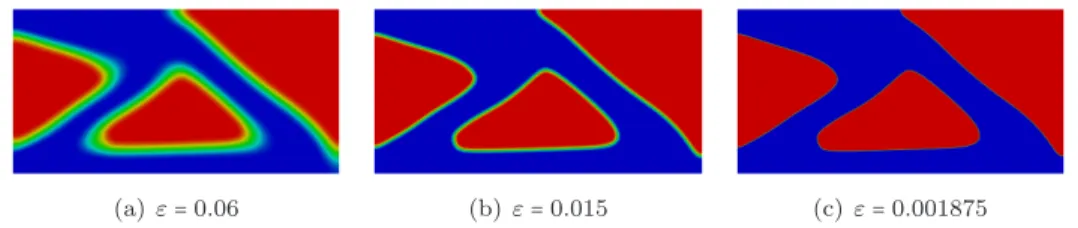
Results for minimizing the mean compliance of a cantilever beam for three dif- ferent phase field parametersεare shown in Figure 3.2. Here we chose the weighting factor for the Ginzburg Landau energyγ=0.5. Already forε=0.06 one obtains the same structure as for the smallest value of the phase field parameter, i.e. the right qualitative behaviour of the sharp interface minimizer. We also remark that for the smallest value ofε, the interface is already very thin and almost not visible anymore.

We want to study the convergence of the minimizers(ϕ_ε)ε. For this purpose we de- note byϕ0 a minimizer for the sharp interface problem. As this minimizer is a priori unknown, we approximate ϕ0 by ˜ϕ0∶=2χ{ϕεmin>0}−1, whereεmin∶=0.001875. Thus the optimal interface Γ0 is approximated by the zero level set of ϕ_εmin, denoted by Γ˜0. The difference∥ϕε−ϕ˜0∥L¹(Ω) can be separated into two terms,

∥ϕ_ε−ϕ˜0∥L¹(Ω)∼ ∥ϕ_ε−ϕ^o_ε∥L¹(Ω)+∥ϕ^o_ε−ϕ˜0∥L¹(Ω) (35)

(a) Configuration of the cantilever beam (b) Optimal configuration for γ = 0.002. The stiff material is blue.

Figure 3.1.Cantilever beam

(a) ε=0.06 (b)ε=0.015 (c)ε=0.001875

Figure 3.2.Optimal material configurationϕεfor the cantilever beam forγ=0.5and different values ofε(stiff material in blue, weak material in red and interface in green).

0 0.05 0.1 0.15 0.2 0.25 0.3 0.35 0.4

0 0.01 0.02 0.03 0.04 0.05 0.06

epsilon

L¹error mε

(a) The solid blue line shows∥ϕ^ε−ϕ˜0∥L¹(Ω). The approximated diffuse interface error is de- picted in the red, dashed line.

19.8 20 20.2 20.4 20.6 20.8 21 21.2 21.4 21.6

0 0.01 0.02 0.03 0.04 0.05 0.06

epsilon

Cost functional

(b) The cost functional jε(ϕε)seems to con- verge asε↘0.

−11

−10.5

−10

−9.5

−9

−8.5

0 0.01 0.02 0.03 0.04 0.05 0.06

epsilon

Lambda

(c) The Lagrange multiplierλ^ε seems to con- verge asε↘0.

Figure 3.3.Data corresponding to Figure 3.2.

where (ϕ^o_ε)^ε denotes the constructed recovery sequence corresponding to ˜ϕ0 and ex- poses a sin-profile normal to ˜Γ0, see [15]. We want to determine which term of the error in (35) is the dominating part. We notice that the first term on the right- hand side of (35) can be considered as the distance of the zero level sets ofϕε and ϕεmin and the second term describes the error resulting from the diffuse interface pro- file. The 1D error of the sin-profile compared to a characteristic function is given by ∫^{−επεπ//22}∣sin(^x_ε)−sgn(x)∣dx= (π−2)ε. Thus, the L¹(Ω)-error in our 2D setting can be approximated by ∥ϕ^o_ε−ϕ˜0∥L¹(Ω) ≈ PΩ({ϕ0 = 1})(π−2)ε. As the perimeter PΩ({ϕ0=1})is not known, we extrapolate the given sequence(E_ε(ϕ_ε))εnumerically to ε= 0, which gives limε↘0E_ε(ϕ_ε)≈ e0 ∶= 8.1754. As mentioned above, from the Γ-convergence result of [15, 33] it is expected that e0 ≈ ^π2PΩ({ϕ0= 1}). Hence, we may approximate∥ϕ^o_ε−ϕ˜0∥L¹(Ω)≈mεwithm∶= ^2(π−_π²⁾e0.

In Figure 3.3(a) we depict now the difference∥ϕ_ε−ϕ˜0∥L¹(Ω) (solid blue line) together with the approximated diffuse interface error mε (dashed red line). We see that for ε< 0.02 the L¹-difference of the minimizer ϕ_ε and the approximated minimizer ˜ϕ0

becomes tangential to the line mε. This indicates that the error resulting from the diffuse interface profile dominates the total approximated error in (35) and that the distance of the zero level sets becomes comparably small. Hence, the level set ofϕε

is already forε<0.02 a good approximation of the optimal interface Γ0.

To complete this picture we also give a plot of the minimal functional values jε(ϕε) and the Lagrange multipliers λε for the calculated ε values in Figure 3.3(b) and 3.3(c). One sees that (j_ε(ϕ_ε))^ε is monotonically decreasing as ε decreases and seems to converge linearly to a specific value, supposedly a minimal value forj0, com- pare also Theorem 20. Likewise,(λ_ε)εconverges linearly to a limit valueλ0, compare Theorem 21.

To study the influence of the perimeter penalization, we carried out the same calcula- tions for a smaller weighting factorγ. We can control the appearance of fine structures by the choice ofγ. As an example, we refer to Figure 3.1(b), where we used the pa- rametersγ=0.002,ε=0.001. This verifies numerically that the regularization yields a well-posed problem but still gives desired optimal structures. Moreover, the influence of regularization parameters on the fineness of the structure is in accordance to other methods (see e.g. [8]). For the computation we chose the inner product

ak(ϕ1, ϕ2)∶=γε∫_Ω∇ϕ1⋅ ∇ϕ2dx−2∫_ΩC^′(ϕk)(ϕ1)E(z)∶E(uk)dx,

which depends on the current iterateϕk and which includes second order information of the Ginzburg-Landau energy, as well as of the compliance part. Here, we used uk ∶= S(ϕ_k) and z ∶= S^′(ϕ_k)ϕ2 ∈ H¹_D(Ω) which is given as the solution of the linearized state equation

∫ΩC(ϕk)E(z)∶E(v)dx=−∫ΩC^′(ϕk)ϕ2E(uk)∶E(v)dx+∫Γ_gg⋅vds ∀v∈H¹_D(Ω). 3.3. Optimal material distribution within a wing. We now consider a dif- ferent geometry for the overall container Ω in a three dimensional setting. This example shows that we can also use different geometries, i.e. different choices of Ω, and work in a three dimensional setting.

We perform the same optimization strategy as above and optimize the material con- figuration within a wing of an airplane. This example is to be considered as an

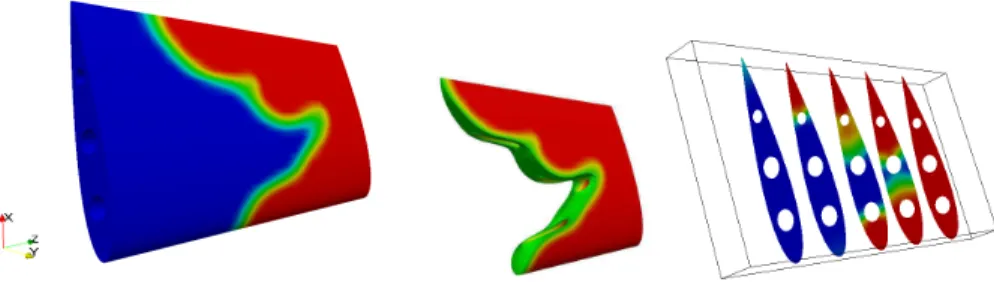
Figure 3.4. Optimal material configuration of a NACA 0018 airfoil wing with 3 holes where blue represents the stiff material.

Figure 3.5.Optimal designs including eigenstrain.

outlook on possible applications. One wants to have a composite material in order to obtain a high ratio of stiffness to weight. Hence we use one very stiff material (λ1 = 5000, µ1 = 5000) and a material representing the light material (λ2 = 100, µ2=100). As geometry we use a three dimensional NACA 0018 airfoil configuration with three holes in it. The configuration can be seen in Figure 3.4.

The considerations of the previous example have shown that we do not have to chooseε too small in order to obtain the right qualitative behaviour and so we use hereε=0.06.

Moreover, the weighting factor for the Ginzburg-Landau regularization is chosen quite small, i.e. γ=10⁻⁴. The boundary forceg(x, y, z)=(0,0.03

√

1−(0.5y)²,0)is of el- liptic form, which is typical for the lift force acting on an airplane wing, compare for instance [23]. Its support is on Γ⁰_g∶={(x, y, z)∈∂Ω∣y>0}. The Dirichlet boundary ΓD = {(x, y, z)∈ ∂Ω∣z =0}is the part where the wing is attached to the airplane (left-hand side in Figure 3.4). The optimized material configuration is shown in Fig- ure 3.4, where the blue material is the stiff material. We also give a picture of the weak material, i.e. the set{ϕε<0}, see Figure 3.4, in order to see the hypersurface separating the two materials, together with various cross sections of the wing.

3.4. Influence of eigenstrain. Left hand side of Figure 3.5: We takeE(ϕ)= δϕI with δ=0.08, ε=0.01 and γ=0.5 and λ1=µ1 =5000 andλ2=µ2 =5 (strong and weak material). Right hand side of Figure 3.5: We takeE(ϕ)=δϕ(−1 0

0 1)with δ=0.01, ε=0.04 andγ=0.5 and λ1=µ1 =λ2=µ2=5000 (homogeneous material).

The rest of the parameters are the same as in Section 3.2.

4. Derivation of the optimality conditions. In this section we will give the proofs of Theorem 12 and Theorem 17. We start with showing the differentiability oft↦(S(ϕ○T_t⁻¹)○Tt) att=0 forT ∈ T^ad and ϕ∈L¹(Ω), ∣ϕ∣≤1 and deriving the