using a phase field approach and an application in structural optimization
DISSERTATION ZUR ERLANGUNG DES DOKTORGRADES DER NATURWISSENSCHAFTEN (Dr. rer. nat.)
DER FAKULT ¨AT F ¨UR MATHEMATIK DER UNIVERSIT ¨AT REGENSBURG
vorgelegt von Claudia Hecht
Regensburg, Januar 2014
Die Arbeit wurde angeleitet von Prof. Dr. H. Garcke.
Pr¨ufungsausschuss: Vorsitzender: Prof. Dr. U. Bunke 1. Gutachter: Prof. Dr. H. Garcke 2. Gutachter: Prof. Dr. H. Abels weiterer Pr¨ufer: Prof. Dr. G. Dolzmann
We consider the problem of shape and topology optimization in fluid mechanics with a general objective functional. A phase field approach is introduced and discussed in terms of well-posedness and first order necessary optimality conditions. The state constraints are either given by the Stokes or the stationary Navier-Stokes equations. We find that minimizers of the diffuse interface setting have a converging subsequence as the interface thickness tends to zero. If this sequence fulfills a certain convergence rate or the total potential power is minimized in a Stokes flow, we obtain that the limit element is a minimizer of the sharp interface formulation. Additionally, we can derive in both, the Stokes and stationary Navier-Stokes setting, optimality conditions of the sharp interface model which can be verified to be the limit of corresponding optimality systems of the phase field model. Finally, we also apply this approach to structural optimization, where we want to find the optimal material distribution of two given elastic materials for a general objective functional. Using the techniques developed before, we can derive convergence results of a phase field approach similar to the fluid mechanical setting and discuss both the diffuse and the sharp interface formulation with regard to well-posedness and necessary optimality conditions.
I want to express my special thanks to my supervisor Prof. Dr. Harald Garcke for giving me the chance to research in such a great field and to learn from his experience.
Thank you for always giving me constant encouragement and providing ideas leading in new directions. I want to thank Prof. Dr. Helmut Abels for taking the time to long discussions and giving me important advices. Further, I have to thank Prof. Dr. Dorin Bucur for showing such a great deal of interest in my work. Our exchange helped me a lot to get a better comprehension of certain problems. I also want to thank Christian Kahle for providing numerical results which gave me a good insight in the problem. I would have missed the long conversations with you. My thanks also go to Prof. Dr. Luise Blank for her support during all the last years and all her advices. I thank all the other colleagues at the University of Regensburg for providing such a nice working atmosphere.
My thanks go to Sabine M¨uller for valuable notes on this thesis. Finally, I want to thank Christoph Rupprecht for all our intense discussions and for always backing and confirming me. Thank you for enriching my life also outside of work.
1 Introduction 11
2 Notation and assumptions 19
3 Mathematical background 28
3.1 Functions of bounded variation . . . 28
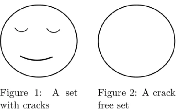
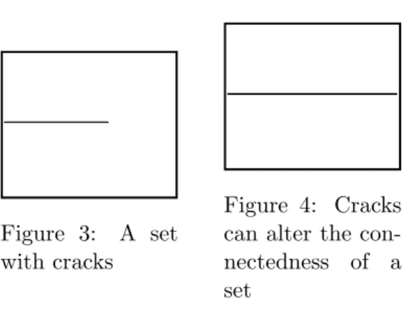
3.2 Crack free Caccioppoli sets . . . 31
3.3 Introduction to shape calculus . . . 33
3.4 Introduction to Γ-convergence . . . 38
I Stokes flow 40 4 Important facts related to fluid mechanics 40 5 Phase field model 42 5.1 Problem formulation . . . 42
5.2 Existence results . . . 44
6 Sharp interface limit 48 6.1 Sharp interface model . . . 48
6.2 Convergence of minimizers . . . 56
6.3 Minimizing the total potential power . . . 63
6.4 Further discussions on possible generalizations . . . 66
7 Optimality conditions for the phase field model 72 7.1 Variational inequality . . . 72
7.2 Geometric variations . . . 82
7.3 Linking the optimality criteria . . . 96
8 Optimality conditions for the sharp interface model 99 8.1 Shape derivative approach . . . 99
8.2 Geometric variations . . . 107
8.3 Linking the optimality criteria . . . 111
9 Convergence of the optimality system 113 10 Examples 121 II Stationary Navier-Stokes flow 123 11 The stationary Navier-Stokes equations 123 11.1 Introduction to known results . . . 123
11.2 Additional assumptions on data and objective functional . . . 128
12.1 Problem formulation . . . 131 12.2 Existence results . . . 132
13 Sharp interface model 136
14 Convergence of minimizers 144
15 Optimality conditions for the phase field model 150 15.1 Variational inequality . . . 150 15.2 Geometric variations . . . 157 15.3 Linking the optimality criteria . . . 163 16 Optimality conditions for the sharp interface model 164 16.1 Shape derivative approach . . . 164 16.2 Geometric variations . . . 171 16.3 Linking the optimality criteria . . . 181
17 Convergence of the optimality system 182
III Pressure functionals in a Stokes flow 186
18 Introduction 186
18.1 Problems using a general objective functional . . . 186 18.2 Possible choices of objective functionals . . . 188
19 Phase field model 194
19.1 Problem formulation . . . 194 19.2 Existence results . . . 195 19.3 Optimality conditions . . . 197
20 Sharp interface model 205
20.1 Considering the pressure in measurable sets . . . 205 20.2 Statement of the sharp interface model . . . 207 20.3 Optimality conditions . . . 209
21 Sharp interface limit 211
21.1 Convergence of minimizers . . . 211 21.2 Convergence of the optimality system . . . 219 22 Pressure functionals in a stationary Navier-Stokes flow 221
IV Application in structural optimization 224
23 Introduction and assumptions 224
24.2 Existence results . . . 231 24.3 Optimality conditions . . . 234
25 Sharp interface model 240
25.1 Problem formulation . . . 240 25.2 Existence results . . . 242 25.3 Optimality conditions . . . 242
26 Sharp interface limit 250
26.1 Γ-convergence of the objective functionals . . . 250 26.2 Convergence of the optimality system . . . 252
Summary and Conclusions 256
Appendix 258
Symbols 260
References 264
1 Introduction
The mathematical problem of shape optimization in fluids is to minimize some objective functional depending on the solution of a system of partial differential equations describ- ing the fluid mechanics in an unknown bounded set. The control is represented by the shape of the set. If the topology of the set is not prescribed in advance, we refer to those problems as shape and topology optimization. Another application of shape and topology optimization can be found in structural optimization. There we try to find an optimal configuration of two different elastic materials in some fixed container, where optimal once again means that a certain objective functional depending on the behaviour of the elastic materials is minimized.
Applications of shape and topology optimization reach from optimizing guitars, crashwor- thiness of transport vehicles and tunnel design to biomechanical applications such as bone remodelling. Structural optimization has turned out to be helpful in solving automative design problems in order to maximize the stiffness of vehicles for instance or reduce the stresses to improve durability. In the context of fluid mechanics, we can find utilizations in the paper production industry ([HMT99]) or in biomedical engineering such as consid- ering blood flow or the study of lungs and kidneys ([ABH05, BBB+12, Bej00]). Moreover, we find a lot of work done in car design using the ideas of shape optimization in fluid dynamics, see for instance [GO05, DHM04, HS93, HH09]. However, it seems that airplane optimization plays the biggest role in applications, in particular in terms of optimization of wings and airfoils. A small percentage of a wing’s drag minimization already yields a large profit for the industry. Just to mention a few works recently done on this topic we refer to [MP01, HMTT00, JMP98, Ang83, JMP98, GISS12, SSS11] and also to exist- ing software like [BNS09, FD12]. In fact, there are many more application fields and we mention for instance the overviews in [MP04, Ben03, HM03, JT08, Bej00].
Newton already discussed the problem of finding the shape of an object’s surface in a fluid having the least resistance, which can be considered as a first study of the drag minimizing problem, see [New63]. Nowadays, applications of this problem may be seeking the optimal shape of a harbor, while trying to minimize the incoming waves or optimizing wings or airfoils of an airplane as mentioned above. Another classical example in the field of finding optimal geometric forms, although not in fluid dynamics, is Plateau’s problem, which consists of finding a set of least area among all sets with a given boundary and is motivated by Plateau’s experiments with soap films. One important contribution con- cerning this problem was made by De Giorgi, see [DG61], by considering this problem in the context of sets of finite perimeter. He was one main contributor to the theory of sets of finite perimeter, also known as Caccioppoli sets, see [DG54]. Caccioppoli sets define the framework for our sharp interface model, too. Thus the fluid region, which will be the control in our problem, is chosen to be a Caccioppoli set. Using Caccioppoli sets as admissible space in shape optimization is a commonly used approach, see for instance [DZ01, SZ92, AB93, BHJ96].
One of the first treatments of shape optimization in a general setting appeared in [CZ73], where a finite element model is introduced. For a good review of the first approaches towards shape optimization we refer to [CH81]. In the context of optimal control the- ory, thus having partial differential equations as part of the model, the first discussions
of topology optimization were mainly aimed at structural optimization in elastic bod- ies, see for instance [BK88, KS86, EO01, Ben03, HP05] and included references. One of the first approaches of finding the optimal material distribution in presence of two materials can be found in [Tho92]. But the problem of finding optimal structures in mechanical engineering dates at least back to the beginning of the 20th century where Michell [Mic04] considered optimal truss layouts. In the field of fluid mechanics there are mainly works considering optimal shapes, while fixing the topology. Pioneering works in this branch were in particular [Pir73, Pir74, Sim91, Sim80] and we refer to [MP04, GI04, DZ01, HM03, SS10, PS10, JLM03] for some recent works. Most of those works concentrate on numerical methods or on local deformation of some given fluid do- main and calculating shape derivatives. One of the typical examples considered there is the drag minimizing problem. Regarding the general problem of finding the optimal form of a fluid region to minimize a given cost functional, the approach of pure shape optimiza- tion with fixed topology may not be the best choice, since the optimal topology is a priori unknown. As indicated in our numerical examples in Section 10, it is for instance not clear how many pipes are optimal to transport a fluid. Thus topological changes should be allowed to get optimal profiles, which leads to the field of topology optimization in fluid dynamics.
This is still a young research field receiving growing attention in recent years. One of the first models for treating topology optimization in fluids has been introduced by [BP03]
and is described below. For some recent results on specific topics of topology optimization in fluid dynamics we refer for instance to [DLL+11, GHHS05, KMP11, BKW07, Wik08], which mainly concentrate on numerical aspects and on the discussion of the model intro- duced in [BP03]. In the work of [BP03] the Stokes equations describe the fluid and the minimized objective functional is the drag functional. Moreover, an additional penaliza- tion termα, which is called inverse permeability, is introduced both in the state equations and in the objective functional. The Stokes equations then read in the strong formulation
α(ρ)u−µ∆u+ ∇p=f, divu=0 and the corresponding objective functional is given by
1
2∫Ωα(ρ) ∣u∣2 dx+ ∫Ω µ
2 ∣∇u∣2−f⋅udx.
This penalization termα should be very small in the fluid region, and very large outside, so that the velocityuvanishes in the limit outside of the fluid region. The design variable ρ is then a function with values between 0 and 1, where 0 corresponds to non-presence of fluid and 1 to the presence of fluid. We will use a similar approach in this work. In [BP03]
the inverse permeabilityαis a fixed function, interpolating between two fixed finite values.
We will consider the case, that the interpolation function αε depends on some parameter ε > 0, and as ε ↘ 0 the penalization term will vanish in the fluid domain, and will be infinite outside of the fluid. If αε is interpreted as inverse permeability of some porous medium outside the fluid this means that the permeability of the porous material tends to zero as ε↘ 0. In [Evg05] the finiteness and fixed choice of α is interpreted as “not allowing real topology changes of the fluid region”, since the permeability of the porous medium is never zero, thus no “real walls” can appear. In our sharp interface model, the permeability of the porous material will be zero and so, following the definition of
[Evg05], we allow “real” topology changes. Another discussion of topology optimization in fluids can be found in [Evg05, Evg06]. There, the same model as in [BP03] is con- sidered, but the interpolation function α now interpolates between zero and infinity, and thus giving rise to “real” topological changes. Moreover, the existence of black-and-white solutions (thus there exist only fluid or non-fluid regions, and no values in between) is shown. Yet, there are drawbacks in their work. Using the approach of [Evg05], it is not clear if this problem is still well-posed in case of objective functionals other than the drag functional. Moreover, the convergence of dark-grey-and-light-grey solutions (thus for the design variable only values close to 0 and close to 1 exist) to black-and-white solutions in the strong topology can only be shown under some additional assumption. Additionally, it is indicated in [Evg05] that numerics may pose problems in this setting.
As it turns out, none of the problems mentioned above arise in our approach. Since we approximate the black-and-white solutions by a diffuse interface problem, namely a phase field approach, numerics can be carried out with known techniques and existence of the approximating problem can even be ensured with a general objective functional. The con- vergence of the diffuse interface solutions to the sharp interface black-and-white solutions in the strong L1-topology can be shown for the problem of minimizing the total poten- tial power without additional assumptions. Besides, we can consider a general objective functional and under certain assumption we can still prove convergence of minimizers.
Moreover, the approach of [Evg05] could not directly be generalized to the stationary Navier-Stokes equations, see [Evg06], but instead a relaxation of the incompressibility constraint and a filter have to be introduced in order to get a well-posed problem. Again this is no problem in our approach and we can handle the nonlinear state equations with- out major changes in the model.
We suggest a phase field model to describe the topology optimization problem. The idea is to have a small interfacial layer between the fluid region and the region outside the fluid, rather than the boundary of the fluid region being a free hypersurface. Phase field models are currently widely used in different research fields. The diffuse interface approach was already proposed by van der Waals [vdW79]. Later on, this theory was gen- eralized by Ginzburg and Landau [GL50], and researches like Cahn, Hilliard and Allen, see [CH58, AC79, Cah61, CH59], applied it to microstructural evolution processes like spinodal decomposition and domain coarsening kinetics in binary alloys. Recently, appli- cations of phase field models can be found in fields like phase transformations, solidification processes, grain growth and lately also in image segmentation, see for instance [BCM04].
For a good review we refer to [Che02]. Finally, phase field models were also coupled to hydrodynamic models and have for example applications in binary mixtures [LT98], spin- odal decomposition, mixing and interfacial stretching or nucleation of droplets. A good overview can be found in [AMW98, LT98].
One of the first researchers using a phase field formulation for topology optimization were Bourdin and Chambolle in [BC03], where the compliance is minimized while regulariz- ing with a perimeter term. After introducing a so-called fictious material relaxation, the perimeter is approximated by the Ginzburg-Landau energy, and Γ-convergence of the re- sulting energy is shown. In the main part of this thesis, we will consider fluid dynamics, which already implies a different setting as in [BC03]. Besides, our approach for shape op- timization in fluid mechanics regularizes the state equations and the perimeter functional
at the same time. In [BC03], Γ-convergence of their reduced objective functional was proven by using the Γ-convergence result of Modica and Mortola [Mod87, MM77] and by showing that their functional is a continuous perturbation of the Ginzburg-Landau energy. However, this strategy cannot be used in our setting, because we have a problem in which both the objective functional and the state constraints depend on the phase field parameter ε>0. In the last part we will apply the techniques developed before to struc- tural optimization. There, the state equations are independent of the phase field variable ε>0, but in contrast to [BC03] we consider a general objective functional and in addition to Γ-convergence of the reduced objective functionals we can show that certain first opti- mality systems of the phase field problem converge to necessary optimality conditions of the sharp interface formulation. So far, similar considerations have only been carried out by formal asymptotics, compare [BFSGS13]. For further results on applications of phase field models in topology optimization we refer to [WZ04, BGS+12, KNT10, BC06]. To the author’s knowledge, a phase field approach has not been applied to topology optimization in fluids before.
One major advantage of our phase field approach for topology optimization is the regu- larity of the phase field variable describing the fluid region, which allows more efficient numerical calculations and gives rise to better analysis, while providing all relevant geo- metric properties. Moreover, topological changes can be handled without much effort, as well as numerics can be carried out quite easily, since we can apply the well-developed methods for phase field models. Besides, parametrization of a fixed domain by a family of diffeomorphisms, as it is done for instance in [AJ05, MP04, NPT09, MP01], naturally limits the admissible solutions. Using a phase field approach we certainly enlarge the set of possible solutions. Since we can show that the phase field formulation yields an appropriate approximation for the sharp interface problem, it is a serious alternative in this setting. In particular, most of the classical shape calculus results cannot be carried out rigorously, since the lack of regularity of the minimizing sets result in heuristic calcu- lations and well-posedness, thus the existence of minimizers, is often not guaranteed. Our results are all verified and consistent without imposing unverified assumptions and give rise to a more systematic approach to topology optimization in fluid dynamics. But if the assumptions necessary for deriving the classical shape optimization results are fulfilled, we can show that our first order optimality condition results are equivalent to those of the known literature, see for instance [BFCLS97, BFCLS96, GMZ08, MP04, Pir73, Pir74, Sim91, SS10, ADDM13, AJVG11, HHS13].
In the main part of this study, we will consider a general objective functional depending on the velocity uof some fluid (Part I and II), namely
∫Ωf(x,u,Du)dx.
In the third part it can additionally depend on the pressurepof the fluid, thus we minimize
∫Ωf(x,u,Du)dx+ ∫Ωh(p)dx.
We handle this case in a separate part because certain difficulties occur, see also discussion in Section 18.1. The state equations are either the Stokes equations (Part I and III), given
in the strong formulation by
−µ∆u+ ∇p=f, divu=0,
or the stationary Navier-Stokes equations (Part II and discussion at the end of Part III) which are given by
−µ∆u+u⋅ ∇u+ ∇p=f, divu=0.
We will show that our phase field approach is a good approximation of the sharp interface model in the sense that minimizers of the phase field formulation converge to a minimizer of the sharp interface setting under certain assumptions. In the particular situation of minimizing the total potential power in a Stokes flow we can even prove Γ-convergence of the reduced objective functionals. The sharp interface formulation is, as already men- tioned above, a topology optimization problem where the admissible sets are Caccioppoli sets and the objective functional is penalized by adding a perimeter term PΩ(E), which is the perimeter of the fluid regionE inside the fixed container Ω. This perimeter penal- ization is a typical ansatz to overcome the general ill-posedness of the problem, see for instance [Pet99, AB93, BC03, Mur77].
The notion of Γ-convergence was introduced by De Giorgi [DG75] and has since been extended to a broad range of applications. One of the most important results concerning Γ-convergence of functionals is certainly the result of Modica and Mortola [MM77, Mod87], who proved that the Ginzburg-Landau energy
Eε(ϕ) = ∫Ωε
2∣∇ϕ∣2+1
εψ(ϕ)dx Γ-converges to some multiple of the perimeter functional
PΩ({ϕ=1})
inL1(Ω) asε↘0, compare also the results in [Ste88, Alb00]. This will be an important ingredient for our approach, too, since the phase field models presented in this thesis will have the Ginzburg-Landau energy as a penalization term in the objective functional and the sharp interface problems contain the perimeter functional. Γ-convergence results have already been discussed for phase field approaches in topology optimization of ma- terials, where we mainly point out the work of [BC03, WZ04, Gar08, PRW11]. In the last part, where we consider structural optimization, we state comparable results as in [BC03, WZ04] concerning Γ-convergence of the reduced objective functionals but with a very generally formulated problem.
We emphasize that in the fluid dynamical problems considered here, the state equations depend on the phase field parameter ε, which describes the interface thickness. This is not the case in the cited works above, but changes the mathematical considerations dras- tically.
In the specific setting of minimizing the total potential power in a Stokes flow we will prove Γ-convergence of the reduced objective functionals. For a general objective functional and the stationary Navier-Stokes equations, we can show under certain assumptions on the sequence of minimizers of the phase field problems that those minimizers approximate a minimizer of the sharp interface problem. We can even show that certain first order optimality conditions of the phase field model and the sharp interface model converge to
each other, both in the fluid dynamical problems and in structural optimization. This is an important result and has to the author’s knowledge not been shown in a comparable setting before.
One aim of this work is to show well-posedness of the phase field approach and to show that it approximates the classical topology optimization problem, which is a sharp inter- face model. Additionally, we derive first order necessary optimality conditions for both models and show that the optimality system derived in the diffuse interface model ap- proximates the optimality system of the sharp interface model.
This dissertation is organized in four parts as follows:
Part I: In the first part, we start by considering a general shape and topology optimiza- tion problem, where the objective functional depends on the velocity of the fluid described by the Stokes equations. We first introduce the phase field approach de- scribing the shape and topology optimization problem on a diffuse interface level in Section 5. After discussing well-posedness of this problem, we formulate the sharp interface shape and topology optimization problem in Section 6, discuss its well- posedness, and show that minimizers of the phase field model have a converging subsequence if the interface thickness tends to zero. If this converging subsequence fulfills a certain convergence rate, we find that the limit element is a minimizer of the sharp interface model and that the minimal functional values converge, too. In the specific situation of minimizing the total potential power we can even obtain the stronger result of Γ-convergence of the reduced objective functionals associated to the phase field problems, see Section 6.3. Finally, we discuss in Section 6.4 possible extensions of the obtained statements and whether a more general result could be expected.
To discuss first order optimality conditions we first derive the classical variational inequality for the phase field model in Section 7.1 by parametric variations. But we also vary the design variable in Section 7.2, which is the phase field variable in this approach, by deforming the domain with a suitable transformation. Thus we apply the same idea as used in shape calculus. This will lead to suitable optimality conditions that approximate the optimality conditions of the sharp interface model.
Moreover, we can show that under suitable assumptions those conditions can also be derived from the variational inequality directly, see Section 7.3.
Similarly, we start discussing optimality conditions for the sharp interface model in Section 8. First of all we calculate shape derivatives in Section 8.1, while assuming more regularity on the minimizer than we can actually prove. We remark that those regularity assumptions are typically imposed in the field of shape calculus. As a result we see that we arrive in the same results as already known in literature. Then we generalize this result by calculating first order optimality conditions, that can be shown without additional assumptions, see Section 8.2, but are under suitable as- sumptions equivalent to the shape derivatives calculated before, compare Section 8.3.
Finally, in Section 9 we even show that the optimality conditions of the phase field model derived in Section 7.2 converge, as the thickness of the interface tends to zero,
to the optimality conditions of the sharp interface model derived in Section 8.2 if the convergence rate on the sequence of minimizers mentioned above is satisfied.
Thus we have obtained a consistent approximation of the sharp interface model by means of our phase field approach.
Part II: In the second part we consider the stationary Navier-Stokes equations as a sys- tem describing the fluid motion, while still regarding the general objective functional depending on the velocity of the fluid that has been considered in the first part. Due to the fact that uniqueness of a solution to the stationary Navier-Stokes equations can only be shown under additional assumptions, we have to impose some restric- tions on the objective functional in Section 11.2, which are for instance in case of the drag minimization problem equivalent to “smallness of data or large viscosity”, as in classical results. After that we introduce the phase field model and discuss its well-posedness, see Section 12. In Section 13 we consider the sharp interface model and examine the state equations with regard to solvability and uniqueness. Analo- gously to the first part we show that there exists a subsequence of the sequence of minimizers of the phase field problems, that converges as the thickness of the inter- face tends to zero. Assuming this subsequence satisfies a certain convergence rate we prove that the limit element is a minimizer of the sharp interface model in Section 14.
Then we derive first order optimality conditions for the phase field model in Sec- tion 15, first in form of a variational inequality, and then again by varying the domain by means of a transformation, and show thereafter that we can directly de- rive the latter from the variational inequality, too. Then we calculate classical shape derivatives of the sharp interface problem in Section 16.1, while imposing additional regularity assumptions on a minimizing set, that have not been verified in general.
But we can derive optimality conditions without stating additional assumptions in Section 16.2, and show that those are equivalent to the results obtained by shape calculus if imposing the regularity assumptions used in Section 16.1.
We complete the discussion in Section 17 by showing that the optimality system of the diffuse interface model approximates optimality conditions of the sharp interface model if the convergence rate stated above is satisfied for the sequence of minimizers.
Part III: In Part III we generalize the objective functional of the previous parts by adding a pressure depending term. The main discussion is carried out while assum- ing the Stokes equations as a fluid model, but in Section 22 we point out that we could also apply the same generalized objective functional to a Navier-Stokes setting as in Part II.
At the beginning, we discuss the correct formulation of the model in this setting, see Section 18.1. Then we examine the phase field model with regard to well-posedness and optimality conditions in Section 19. The same discussion is carried out for the sharp interface model in Section 20, where in addition we briefly consider the general well-posedness of the pressure in measurable sets in Section 20.1.
After discussing both models independently, in Section 21 we prove convergence of minimizers of the phase field model to a minimizer of the sharp interface model
if the interface thickness tends to zero under the constraint that the sequence of minimizers fulfills a certain convergence rate. Besides, we show convergence of the optimality system as in the previous parts.
Part IV: In the last part, we will apply the methods and techniques developed before to a rather general problem in structural optimization. To be more precise, the problem is to find an optimal configuration in a mixture of two elastic materials. The first discussions are concerned with the formulation and mathematical considerations of an appropriate phase field approach for this problem, see Section 24. In Section 25 we introduce the corresponding sharp interface problem. In contrast to the fluid dynamical problems examined in the first three parts of this work, we can even directly show existence of a minimizer for the sharp interface problem. Besides, we use the ideas of the previous parts to obtain first order optimality conditions by geometric variations for both the sharp and the diffuse model. The subject of Section 26 is to connect the phase field formulation to the sharp interface problem.
This is first done in terms of Γ-convergence of the reduced objective functionals. We remark that this is possible here without additional assumptions on the convergence rate of the minimizers or on the specific form of the objective functionals, as it was necessary in the first parts. Finally, we also prove that the first order optimality conditions for the phase field model derived before by geometric variations are an approximation of necessary optimality conditions in the sharp interface setting. In particular, we hereby generalise findings from literature where this result has already been indicated by formal asymptotics for certain objective functionals.
2 Notation and assumptions
We start our discussion by introducing some notation that we will use in the following and by giving the general assumptions that have to be fulfilled throughout the first three parts in this work, if not stated differently. In the last part we are considering struc- tural optimization, thus the general setting changes in comparison to the first three parts where the problems are based upon fluid mechanics. Thus we will change the setting in the last part and details concerning this notation and assumptions can be found in Section 23.
First of all we define the fixed domain Ω, which will be some container in the following discussion, and the external forces that are given in this setting.
(A1) Ω ⊆ Rd is a bounded Lipschitz domain with outer unit normal n and d∈ {2,3}, such thatRd∖Ω is connected.
(A2) External forces:
f ∈L2(Ω) is the applied body force andg∈H12(∂Ω) the given boundary function such that∫∂Ωg⋅ndx=0.
We will propose a phase field model that approximates the sharp interface topology opti- mization problem. Therefore, we approximate the perimeter functional by the Ginzburg- Landau energy, where we still have to choose the potential that is used in this energy.
Here we will focus on a double obstacle potential, leading to a so-called “sharp-diffuse”
interface. For further discussions of different potentials we refer to [BE91].
(A3) Potential:
ψis assumed to be an obstacle potential of the following form:
ψ∶R→R, ψ(ϕ) ∶=⎧⎪⎪
⎨⎪⎪⎩
ψ0(ϕ), if ∣ϕ∣ ≤1 +∞, if ∣ϕ∣ >1 where
ψ0(ϕ) ∶= 1
2(1−ϕ2).
Let us denote byR∶=R∪ {±∞} the extended real numbers equipped with the standard order topology together with the usual convention 0−1= ∞ and ∞ ⋅0=0.
Moreover, we introduce an interpolation function αε as in [BP03], which appears in our phase field model in the objective functional and in the state equations. This interpolation function can be considered as inverse permeability, as it will have large values outside the fluid region (namely αε(−1) =αε) and will be zero in the fluid region (modelled by αε(1) = 0), where we remark that our design variable ϕ will have values 1 in the fluid region and -1 outside of the fluid. This inverse permeability can be considered, as the name already indicates, as inverse permeability of some porous medium being located outside the fluid. Hence, in the pure non-fluid domain, the state equation can be considered as a Darcy flow through porous medium with permeabilityα−ε1. In the pure fluid phase, we will obtain the classical Stokes equations or Navier-Stokes equations, depending on the
model. Moreover, we ensure by adding a term including αε to the objective functional that the velocity of the fluid is zero outside the fluid domain in the limit case ε↘0. A more detailed description of the phase field approach can be found in Section 5.1.
One important property is that αε depends on the phase field parameter εthat models the thickness of the interface, and as εtends to zero, αε will interpolate between infinity and zero, thus allowing “real” walls and topological changes, compare also discussion in [BP03, Evg05, Evg06].
(A4) Inverse permeability/interpolation function:
Letαε∶ [−1,1] → [0, αε] be a decreasing, surjective and twice continuously differen- tiable function for ε>0.
Let α0 ∶ [−1,1] → [0,+∞]be given as a decreasing, surjective, continuous function with α0(0) < +∞.
It is required that αε > 0 is chosen such that limε↘0αε = +∞ and αε converges pointwise to α0. Additionally, we impose αδ(x) ≥αε(x) if δ ≤ ε for all x ∈ [−1,1] and a growth condition of the form αε=o(ε−2/3).
Remark 2.1. In space dimension d= 2 one could weaken the growth condition for αε
stated in Assumption (A4). Applying the imbedding theoremH1(Ω) ↪Lp(Ω) for all p<
∞ we could establish the same results by only imposingαε=o(ε−1+δ)for some δ∈ (0,1), see also Remark 6.3.
We denote Rd-valued functions and spaces consisting of Rd-valued functions in boldface.
Let us introduce the following function space:
U ∶= {u∈H1(Ω) ∣u=g on ∂Ω,divu=0} and the corresponding homogeneous space:
V ∶= {v∈H10(Ω) ∣ divv=0}.
Throughout this work, we will sometimes work with the following auxiliary spaces:
H1g(Ω) = {u∈H1(Ω) ∣u=g on∂Ω}
and
L20(Ω) = {q∈L2(Ω) ∣ ∫Ωqdx=0}.
We will be considering a general objective functional depending on the velocity of the fluid and its derivative in the first two parts. Our basic assumptions on this objective functional are the following:
(A5) Objective functional:
We choosef ∶Ω×Rd×Rd×d→Ras a Carath´eodory function, thus fulfilling i) f(⋅, v, A) ∶Ω→Ris measurable for each v∈Rd,A∈Rd×d, and
ii) f(x,⋅,⋅) ∶Rd×Rd×d→Ris continuous for almost every x∈Ω.
Letp≥2 for d=2 and 2≤p≤2d/d−2 ford=3 and assume that there are a∈L1(Ω), b1, b2∈L∞(Ω) such that for almost everyx∈Ω it holds
∣f(x, v, A)∣ ≤a(x) +b1(x)∣v∣p+b2(x) ∣A∣2, ∀v∈Rd, A∈Rd×d. (2.1) Additionally, assume that the functional
F ∶H1(Ω) →R
F(u) ∶= ∫Ωf(x,u(x),Du(x))dx (2.2) is weakly lower semicontinuous, F∣U is bounded from below, andF is radially un- bounded in U, which means
klim→∞∥uk∥H1(Ω)= +∞ Ô⇒ lim
k→∞F(uk) = +∞ (2.3)
for any sequence(uk)k∈N⊆U.
Remark 2.2. Remark that condition (2.1)implies that H1(Ω) ∋u↦ ∫Ωf(x,u,Du(x))dx
is continuous. To be precise, (2.1)is a necessary and sufficient condition such that Lp(Ω)d×L2(Ω)d×d∋ (v, A) ↦f(⋅, v, A) ∈L1(Ω)
is a well-defined Nemytskii operator. If this operator exists as a Nemytskii operator, it is a continuous operator. For details we refer to [AZ90, Tr¨o09, Sho97].
Remark 2.3. Assume that F∣U is bounded from below, where F ∶H1(Ω) →R is defined in (2.2), and that f∶Ω×Rd×Rd×d→R is smooth. Then the convexity of
Rd×d∋A↦f(x, v, A) ∈R
is according to [Eva98, Theorem 1, Chapter 8.2] sufficient for the weakly lower semicon- tinuity of F.
Besides, the coercivity of F∣U, i.e.
∃c1, c2>0∶ F(u) ≥c1∥Du∥2L2(Ω)−c2 ∀u∈U, is sufficient for (2.3).
The assumptions stated above are the basic assumptions used throughout this work.
When deriving optimality conditions we need to impose more regularity on the objective functional and the external force term, such that we can differentiate:
Additional assumptions necessary for Sections 7-9, 15-17, 19.3, 20.3 and 21.2:
(A6) External body force:
Assume f ∈H1(Ω). (A7) Objective functional:
Assume that x ↦ f(x, v, A) ∈ R is in W1,1(Ω) for all (v, A) ∈ Rd,Rd×d and the partial derivatives D2f(x,⋅, A), D3f(x, v,⋅) exist for all v∈ Rd,A ∈Rd×d and a.e.
x ∈ Ω. Let p ≥ 2 for d= 2 and 2≤ p ≤2d/d−2 for d=3 and assume that there are ˆ
a∈L1(Ω), ˆb1,ˆb2∈L∞(Ω) such that for almost everyx∈Ω it holds
D(2,3)f(x, v, A) ≤aˆ(x) +ˆb1(x) ∣v∣p−1+ˆb2(x) ∣A∣ ∀v∈Rd, A∈Rd×d. (2.4) Remark 2.4. Notice, that the exponentp≥2in Assumption(A5)and Assumption(A7) is chosen in dependency of the space dimension d ∈ {2,3} such that such that H1(Ω) imbeds continuously into Lp(Ω).
Notation Here and subsequently, we will use the notation D(2,3)f(x, v, A) and
Dif(x, v, A) i∈ {1,2,3}
as the differential of
Rd×Rd×d∋ (v, A) ↦f(x, v, A) for fixed x∈Ω and of
Ω×Rd×Rd×d∋ (x,v, A) ↦f(x,v, A) with respect to the i-th variable, respectively, whereas we write
Duf(x,u,Du)v∶=D(2,3)f(x,u,Du) (v,Dv). Remark 2.5. We notice that
Lp(Ω)d∋v↦D2f(⋅, v, A) ∈Lp/p−1(Ω) ∀A∈L2(Ω)d×d L2(Ω)d×d∋A↦D3f(⋅, v, A) ∈L2(Ω) ∀v∈Lp(Ω)d
are well-defined Nemytskii operators if and only if (2.4) is fulfilled. In this case we also obtain that the operator
Lp(Ω)d×L2(Ω)d×d∋ (v, A) ↦f(⋅, v, A) ∈L1(Ω)
is continuously Fr´echet differentiable. And so, if the objective functional fulfills addition- ally Assumption (A7), we find that
F∶H1(Ω) ∋u↦ ∫Ωf(x,u,Du) dx
is continuously Fr´echet differentiable and that its directional derivative is given in the following form:
DF(u)(v) = ∫ΩD(2,3)f(x,u,Du) (v,Dv) dx ∀u,v∈H1(Ω). For details concerning Nemytskii operators we refer to [AZ90, Tr¨o09, Sho97].
The design variable in the phase field model will be a functionϕ∶Ω→Rhaving H1(Ω)- regularity in order to have a derivative which is inL2(Ω). This ensures that the Ginzburg- Landau energy, given by ∫Ω
ε
2∣∇ϕ∣2+ 1εψ(ϕ)dx, which will be part of the objective func- tional, is finite. We impose additionally an integral constraint, thus ⨏Ωϕdx≤β for some fixed constantβ ∈ (−1,1), where we denote by ⨏Ωϕdx∶= ∣Ω∣−1∫Ωϕdx the mean value of ϕ in Ω. This means, that we prescribe a maximal amount of fluid that can be used in the shape and topology optimization process. This condition could without much effort be replaced by a condition of the form ⨏Ωϕdx=β, or by imposing both a maximal and a minimal value−β1 ≤ ⨏Ωϕdx≤β2 withβ1, β2∈ (−1,1).
Due to the choice of the double obstacle potential in the Ginzburg-Landau energy, we have additionally the constraint for the phase field variable to be between -1 and 1, and thus we arrive in the following admissible set for the optimal control problem in the phase field formulation:
Φad∶= {ϕ∈H1(Ω) ∣ ⨏Ωϕdx≤β,∣ϕ∣ ≤1 a.e. in Ω} for some fixed constantβ∈ (−1,1).
Since we will introduce a Lagrange multiplier for the integral constraint, we use the enlarged admissible set
Φad = {ϕ∈H1(Ω) ∣ ∣ϕ∣ ≤1 a.e. in Ω}
for necessary optimality conditions of first order.
To formulate the sharp interface model, we have to introduce some notation. Therefore, letE⊂Ω be some measurable set. Then we define
UE ∶= {u∈U ∣u=0 a.e. in Ω∖E}
where this may be an empty set, for example in the case thatHd−1({g≠0} ∩ (Ω∖E)) >0.
To continue, we denote by
VE ∶= {v∈V ∣v=0 a.e. in Ω∖E} the corresponding homogeneous vector space.
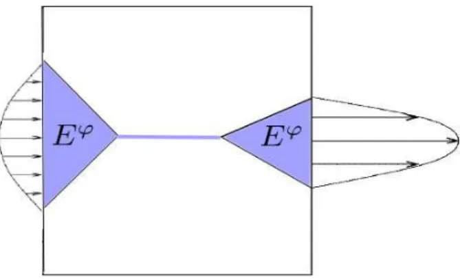
Ifϕis an element in L1(Ω), we see that
Eϕ∶= {x∈Ω∣ϕ(x) =1} is a measurable set and so we can introduce the notation
Uϕ∶=UEϕ and Vϕ ∶=VEϕ.
The corresponding admissible sets of the optimization problem in the sharp interface model are then defined as follows:
Φ0ad∶= {ϕ∈BV (Ω,{±1}) ∣ ⨏Ωϕdx≤β, Uϕ≠ ∅}
and
Φ0ad ∶= {ϕ∈BV (Ω,{±1}) ∣Uϕ≠ ∅}.
The additional constraint Uϕ≠ ∅ is necessary, since for a general ϕ∈BV (Ω,{±1}) this space may be empty, for instance if the prescribed boundary data and the condition u∣Ω∖Eϕ =0 are conflicting, as already mentioned above.
Now we can introduce the functionals that we will be considering in the following and whose minimization defines the topology optimization problem. In the phase field model the objective functional, depending on the phase field parameter ε>0, is defined by
Jε∶L1(Ω) ×H1(Ω) →R
Jε(ϕ,u) ∶=1
2∫Ωαε(ϕ) ∣u∣2 dx+ ∫Ωf(x,u,Du)dx+γε
2 ∫Ω∣∇ϕ∣2 dx+γ
ε∫Ωψ(ϕ)dx (2.5) ifϕ∈Φad andu=Sε(ϕ)andJε(ϕ,u) ∶= +∞otherwise. The solution operator Sε for the penalized Stokes equations is defined in Lemma 5.1.
Moreover, we will see in Section 6.2 that minimizers of the reduced functionals jε∶L1(Ω) →R, jε(ϕ) ∶=Jε(ϕ,Sε(ϕ))
converge asε↘0 under certain assumptions to a minimizer of j0∶L1(Ω) →R, j0(ϕ) ∶=J0(ϕ,S0(ϕ)) where J0∶L1(Ω) ×H1(Ω) →Ris defined as
J0(ϕ,u) ∶=⎧⎪⎪
⎨⎪⎪⎩
∫Ωf(x,u,Du)dx+γc0PΩ(Eϕ) ifϕ∈Φ0ad andu=S0(ϕ),
+∞ otherwise. (2.6)
We remark that the solution operator for the Stokes equationsS0is defined in Lemma 6.1.
In the second part, we will consider the stationary Navier-Stokes equations instead of the Stokes equations as state constraints. Analogously, we then define
JεN ∶L1(Ω) ×H1(Ω) →R JεN(ϕ,u) ∶= 1
2∫Ωαε(ϕ) ∣u∣2 dx+ ∫Ωf(x,u,Du)dx+γε
2 ∫Ω∣∇ϕ∣2 dx+γ
ε∫Ωψ(ϕ)dx (2.7) if u ∈ SNε (ϕ) and ϕ ∈ Φad, and JεN(ϕ,u) = +∞ otherwise, where SNε is the solution operator for the penalized stationary Navier-Stokes equations defined in Lemma 12.1. We will see that those equations may not be uniquely solvable, and so the solution operator
SNε is in general set-valued. Moreover, we will prove in Section 14 that minimizers of (JεN)ε>0 converge under certain assumptions to a minimizer ofJ0N asε↘0, whereJ0N is defined by
J0N ∶L1(Ω) ×H1(Ω) →R
J0N(ϕ,u) ∶=⎧⎪⎪
⎨⎪⎪⎩
∫Ωf(x,u,Du)dx+γc0PΩ(Eϕ) ifϕ∈Φ0ad and u∈SN0 (ϕ),
+∞ otherwise. (2.8)
Here SN0 is the solution operator for the stationary Navier-Stokes equations defined in Lemma 13.1.
As we will derive in Sections 7.2, 8, 15.2 and 16 first order optimality conditions for minimizers of Jε and J0, or JεN and J0N, respectively, by varying the domain Ω with transformations, we introduce here the admissible transformations and its corresponding velocity fields:
Definition 2.1(Vad,Tad,Vad,Tad). The spaceVad of admissible velocity fields is defined as the set of allV ∈C([−τ, τ];C(Ω,Rd)), whereτ >0 is some fixed, small constant, such that it holds:
(V1) (V1a) V(t,⋅) ∈C2(Ω,Rd),
(V1b) ∃C>0: ∥V (⋅, y) −V(⋅, x)∥C([−τ,τ],Rd)≤C∣x−y∣ ∀x, y∈Ω, (V2) V(t, x) ⋅n(x) =0 on∂Ω,
(V3) divV(t,⋅) =0,
(V4) V(t, x) =0 for a.e. x∈∂Ω withg(x) ≠0.
We will often use the notationV(t) =V(t,⋅).
We say that V is an element in Vad if V ∈ C([−τ, τ];C(Ω,Rd)) fulfills (V1), (V2) and (V4).
Then the space Tad of admissible transformations for the domain is defined as solutions of the ordinary differential equation
∂tTt(x) =V(t, Tt(x)) (2.9a)
T0(x) =x (2.9b)
forV ∈ Vad, which gives some T ∶ (−˜τ ,τ˜) ×Ω→Ω, with 0<τ˜ small enough.
Similarly, we say that a transformation T is in Tad if it solves (2.9) together with some velocity field V which is an element in Vad.
We see then directly thatVad⊆ Vad andTad⊆ Tad.
Remark 2.6. Let V ∈ Vad and T ∈ Vad be the transformation associated to V by (2.9).
ThenT inherits the following properties:
T(⋅, x) ∈C1([−τ ,˜ τ˜],Rd) for allx∈Ω,
∃c>0,∀x, y∈Ω, ∥T(⋅, x) −T(⋅, y)∥C1([−τ ,˜˜τ],Rd)≤c∣x−y∣,
∀t∈ [−τ ,˜ τ˜],x↦Tt(x) =T(t, x) ∶Ω→Ω is bijective,
∀x∈Ω, T−1(⋅, x) ∈C([−τ ,˜ τ˜],Rd),
∃c>0,∀x, y∈Ω, ∥T−1(⋅, x) −T−1(⋅, y)∥C([−τ ,˜˜τ],Rd)≤c∣x−y∣.
This follows from [DZ91, Theorem 2.3, Remark 2.4].
We will discuss the admissible velocities and transformations in more detail in Section 3.3.
Before starting the introduction and discussion of the precise models, we want to give an example for an interpolation function αε fulfilling Assumption (A4):
Example 2.1. Letαε=ε−1/2 and αε(x) ∶= 1
1+x+α−ε1 − 1
2(2+α−ε1)− x 2(2+α−ε1). Then αε converges pointwise in(−1,1) to
α0(x) = 1 1+x−1
4−x 4 as ε↘0 and(A4) is fulfilled.
We give now some examples for objective functionals, for which the assumptions above are fulfilled:
Example 2.2. Typical examples forf would be a tracking-type functional for the velocity f1(x,u,Du) = 1
2∣u−ud(x)∣2+1
2∣Du−Dud(x)∣2 for some given ud∈H1(Ω), or
f2(x,u,Du) = ∣curlu∣2 (see for example [GMZ08]) and
f3(x,u,Du) = ∣curlu∣2+ ∣u−ud(x)∣2.
To see that f2 fulfills (2.3), we use [Tem01, Remark 1.6, Appendix I] or [BF13, Chapter IV], which implies that
∥u∥H1(Ω)≤c0(Ω) ∥curlu∥L2(Ω)+c(g,Ω) ∀u∈U.
Example 2.3. In the following we will often use the following functional:
f(x,u,Du) = µ
2 ∣Du∣2−f(x) ⋅u
wheref is the external force given by Assumption(A2) and µ>0 is the viscosity.
Then minimizing ∫Ω(µ2 ∣∇u∣2−f⋅u)dx can be interpreted as minimizing the total po- tential power, minimizing the viscous drag or minimizing the dissipated power while max- imizing the flow velocities at the applied forces. In the special case f ≡0, the problem can in a Stokes flow also be considered as minimizing the average pressure drop (compare [BP03, Appendix A]).
We will use this example in this thesis to give some explicit formulae for the derived optimality systems. As this is a typical objective functional used for shape optimization in fluids, we thus can compare our calculations to known results, such as [Sim80, SS10, MP04, PS10] et al.
Remark 2.7. Beyond, we give some remarks on why some of the assumptions are nec- essary and when we can drop them:
1. The condition of Rd∖Ω being connected arises due to technical reasons, in par- ticular when defining solenoidal extensions of the boundary data, see for instance Lemma 11.3. Anyhow, we could establish the same result for any bounded Lipschitz domain Ω⊂Rd by using for instance a generalized version of Lemma 11.3, which can be found in [Gal11, Lemma IX.4.2]. But then, we would need additional small- ness assumptions on ∫Γig⋅ndx, if Γi are the connected components of ∂Ω, and on the integral along Γi of the gradient of the fundamental solution of the Laplace’s equation, to guarantee existence and uniqueness of the equations appearing in this work. Anyhow, one could transfer our results to this case. On details concerning this topic we refer the reader to [Gal11].
2. The condition ∫∂Ωg⋅ndx=0 stated in Assumption (A2) is the compatibility con- dition, which is a direct result when stating foru∈H1(Ω) that divu=0as well as u∣∂Ω=g, since we get due to Gauß’ theorem
0= ∫Ω divudx= ∫∂Ωu⋅ndx= ∫∂Ωg⋅ndx.
3. The radially unboundedness of the objective functional stated in(2.3)is not necessary for the well-posedness of the phase field model. But the sharp interface model won’t be well-defined without this assumptions, since we cannot guarantee existence of minimizers if the objective functional does not control the velocity, compare also Remark 6.4.
This property will also play an essential role in the proof of Theorem 6.1, where we show convergence of the minimizers.
3 Mathematical background
3.1 Functions of bounded variation
We give here a brief introduction to the theory of functions of bounded variation. For more details and the proofs of the statements that we use here we refer the reader to the books [AFP00, EG92, Giu77, Pfe12]. We start by stating the basic definitions, which are taken from [AFP00].
Definition 3.1 (Functions of bounded variation, BV(Ω)). We say that ϕ∈L1(Ω) is a function of bounded variation in Ω if the distributional derivative ofϕis representable by a finite Radon measure in Ω, i.e. if
∫Ωϕ∂iφdx= − ∫ΩφdDiϕ ∀φ∈C0∞(Ω), i=1, . . . , d for someRd-valued measure Dϕ= (D1ϕ, . . . ,Ddϕ) in Ω.
The vector space of all functions of bounded variation in Ω is denoted by BV(Ω). Functions in BV(Ω) only having the values 1 or −1 a.e. in Ω will be referred to by BV (Ω,{±1}).
We denote the total variation of the measure Dϕ by∣Dϕ∣, thus it holds
∣Dϕ∣ (E) ∶=sup{∑∞
n=0
∣Dϕ(En)∣ ∣En measurable and pairwise disjoint, E= ⋃∞
n=0
En} for all measurable E⊂Ω.
Moreover we define the norm of a function of bounded variation by
∥ϕ∥BV(Ω)∶= ∥ϕ∥L1(Ω)+ ∣Dϕ∣ (Ω).
In the following, we remark some properties of functions of bounded variation:
Properties. 1. The total variation of some ϕ∈BV(Ω) is given by
∣Dϕ∣ (Ω) =sup{∫Ωϕdivφdx∣φ∈C0∞(Ω)d,∥φ∥∞≤1}
and moreover
BV(Ω) ∋ϕ↦ ∣Dϕ∣ (Ω) is lower semicontinuous with respect to the L1(Ω)-topology.
For the proof of this statement we refer the reader to [AFP00, Proposition 3.6].
2. The spaceBV(Ω) equipped with the norm ∥⋅∥BV(Ω) defines a Banach space and the imbedding
BV(Ω) ↪L1(Ω) is compact. This follows from [AFP00, Theorem 3.23].
3. We say that a sequence (ϕn)n∈N ⊆ BV(Ω) converges weakly-∗ in BV(Ω) to ϕ ∈ BV(Ω), if (ϕn)n∈N converges to ϕ in L1(Ω) and
nlim→∞∫ΩφdDϕn= ∫ΩφdDϕ ∀φ∈C0(Ω).
With this definition, we see that (ϕn)n∈N ⊆ BV(Ω) converges weakly-∗ to ϕ in BV(Ω) if and only if (ϕn)n∈N is bounded in BV(Ω) and converges to ϕ in L1(Ω), see [AFP00, Proposition 3.13].
Now we proceed with defining sets of finite perimeter, which are also called Caccioppoli sets.
Definition 3.2(Sets of finite perimeter, Caccioppoli sets). LetEbe a Lebesgue-measurable set inRd. For any Ω⊆Rdthe perimeter ofEin Ω, denoted byPΩ(E), is the total variation ofχE in Ω, i.e.
PΩ(E) ∶=sup{∫E divφdx∣φ∈C01(Ω)d,∥φ∥∞≤1}.
We say that E is a set of finite perimeter in Ω (or Caccioppoli set) if PΩ(E) < ∞. We state some properties of Caccioppoli sets:
Properties. 1. For any set E of finite perimeter in Ω the distributional derivative DχE of the characteristic function χE is an Rd-valued finite Radon measure in Ω with
PΩ(E) = ∣DχE∣ (Ω) (3.1)
and it holds
∫E divφdx= − ∫ΩνE⋅φd∣DχE∣ ∀φ∈C01(Ω)d
where DχE = νE∣DχE∣ is the polar decomposition of DχE given by the Radon- Nikod´ym theorem (see for instance [AFP00, Corollary 1.29]). Hence,νE∶Ω→R is a ∣DχE∣-measurable function such that∣νE∣ =1 ∣DχE∣-a.e..
We callνE the generalised unit normal for the Caccioppoli set E.
2. We say that the Caccioppoli sets (En)n∈N converge in measure toE in Ω if
nlim→∞∣Ω∩ (En∆E)∣ =0
where the symmetric difference for two setsA, B is defined by A∆B = (A∖B) ∪ (B∖A) = (A∪B) ∖ (A∩B).
This corresponds to L1(Ω)-convergence of the characteristic functions. For more details see [AFP00, Remark 3.37].
3. It holds: PΩ(E) =PΩ(F) if ∣Ω∩ (E∆F)∣ =0 andE ↦PΩ(E) is lower semicontinu- ous with respect to convergence in measure inΩ, see [AFP00, Proposition 3.38].
4. For Lebesgue-measurable sets (En)n∈N with sup
n∈NPΩ(En) < ∞
there exists a subsequence that converges in measure in Ω, since ∣Ω∣ < ∞. The proof of this statement can be found in [AFP00, Theorem 3.39].
5. For a better understanding of the perimeter of some setE we notice that
PΩ(E) = Hd−1(Ω∩∂∗E) (3.2) where ∂∗E is the essential boundary ofE andHd−1 denotes the(d−1)-dimensional Hausdorff measure. For details we refer to [AFP00, Definition 3.60]. We just note, that for an open set E with∂E∩Ω∈C2 it holds ∂∗E∩Ω=∂E∩Ω, see [Pfe12], and thus
PΩ(E) = Hd−1(Ω∩∂E) (3.3)
whereas for a general set E we only have
PΩ(E) ≤ Hd−1(∂E∩Ω).
For a fuller treatment we refer the reader to [EG92, AFP00].
Further, we will at some point later on need the following trace theorem, which is taken from [EG92, Theorem 1, Section 5.3]:
Theorem 3.1. Assume U is bounded, open and has a Lipschitz boundary. Then there exists a bounded linear mapping
T ∶BV(U) →L1(∂U) such that
∫Uϕdivφdx= − ∫UφdDϕ+ ∫∂U(φ⋅ν)T ϕdx for all ϕ∈BV(U) andφ∈C1(Rd,Rd).
The function T ϕ, which is uniquely defined up to sets of measure zero, is called trace of ϕ on∂U.
Another important theorem will be the following, see [AFP00, Theorem 2.39]:
Theorem 3.2(Reshetnyak continuity). Letµ,(µn)n∈NbeRm-valued finite Radon-measures in Ω; if limn→∞∣µn∣ (Ω) = ∣µ∣ (Ω) then
nlim→∞∫Ωf(x, µn
∣µn∣(x)) d∣µn∣ (x) = ∫Ωf(x, µ
∣µ∣(x))d∣µ∣ (x) for every continuous and bounded function f ∶Ω×Sm−1→R.
For proving convergence of minimizers of the phase field model in Section 6.2 and Sec- tion 14, we have to approximate Caccioppoli sets by smooth sets. This is done by applying the following lemma, which is taken from [Mod87, Lemma 1]: