Shape optimization for surface functionals in Navier-Stokes flow using a phase

Universit¨ at Regensburg Mathematik

Shape optimization for surface functionals in Navier-Stokes flow using a phase

field approach

Harald Garcke, Claudia Hecht, Michael Hinze, Christian Kahle and Kei Fong Lam

Preprint Nr. 06/2015

Shape optimization for surface functionals in Navier–Stokes flow using a phase field approach

Harald Garcke ^∗ Claudia Hecht^∗ Michael Hinze ^„ Christian Kahle ^„ Kei Fong Lam^∗

April 22, 2015

Abstract

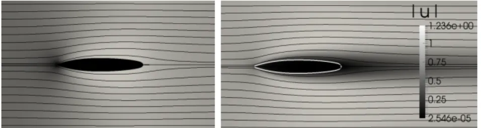
We consider shape and topology optimization for fluids which are governed by the Navier–Stokes equations. Shapes are modelled with the help of a phase field approach and the solid body is relaxed to be a porous medium. The phase field method uses a Ginzburg–Landau functional in order to approximate a perimeter penalization. We focus on surface functionals and carefully introduce a new modelling variant, show existence of minimizers and derive first order necessary conditions. These conditions are related to classical shape derivatives by identifying the sharp interface limit with the help of formally matched asymptotic expansions. Finally, we present numerical computations based on a Cahn–Hilliard type gradient descent which demonstrate that the method can be used to solve shape optimization problems for fluids with the help of the new approach.

Key words. Shape optimization, phase-field method, lift, drag, Navier–Stokes equa- tions.

AMS subject classification. 49Q10, 49Q12, 35Q35, 35R35.

1 Introduction

Shape optimization problems are a very challenging field in mathematical analysis and has attracted more and more attention in the last decade. One of the most discussed and oldest problems is certainly the task of finding the shape of a body inside a fluid having the least resistance. This problem dates back at least to Newton, who proposed this topic in a rotationally symmetric setting. Nowadays, there are a lot of important industrial applications leading to this kind of questions. Among others we mention in particular the problem of optimizing the shape of airplanes, cars and wind turbine blades in order to have least resistance or biomechanical applications like bypass constructions. The wide fields of applications may be one of the reasons that shape optimization problems in fluids received growing attention recently. Nevertheless, those problems turn out to be very challenging and so far no overall mathematical concept has been successful in a general sense.

∗Fakult¨at f¨ur Mathematik, Universit¨at Regensburg, 93040 Regensburg, Germany ({Harald.Garcke, Claudia.Hecht, Kei-Fong.Lam}@mathematik.uni-regensburg.de).

„Schwerpunkt Optimierung und Approximation, Universit¨at Hamburg, Bundesstrasse 55, 20146 Ham- burg, Germany ({Michael.Hinze, Christian.Kahle}@uni-hamburg.de).

…Corresponding author.

One of the main difficulties certainly is that shape optimization problems are often not well-posed, i.e., no minimizer exists, compare for instance [20, 23, 28]. There are some contributions leading to mathematically well-posed problem formulations, see for instance [25], but the geometric restrictions are difficult to handle numerically. The most common approaches used in practice parametrize the boundary of the unknown optimal shape by functions, see for instance [6, 24]. However, those formulations do not inherit a minimizer in general. For numerical simulations typically shape sensitivity analysis is used. Here, one uses local boundary variations in order to find a gradient of the cost function with respect to the design variable, which is in this case the shape of the body.

The necessary calculations are carried out without considering the existence or regularity of a minimizer. But in the end one obtains a mathematical structure that can be used for numerical implementations.

In [14], a phase field approach was introduced for minimizing general volume func- tionals in a Navier–Stokes flow. For this purpose, the porous medium approach proposed by Borrvall and Petersson [4] and a Ginzburg–Landau regularization as in the work of Bourdin and Chambolle [5] were combined. The latter is a diffuse interface approximation of a perimeter regularization. This leads to a model where existence of a minimizer can be guaranteed, and at the same time necessary optimality conditions can be derived and used for numerical simulations, see [15]. In particular, this approach replaces the free boundary Γ of the body B by a diffuse interface. Hence, it is a priori not clear how to deal with objective functionals that are defined on the free boundary Γ.

In this work, we study the following boundary objective functional:

∫Γh(x,∇u, p,ν)dH^d−1, (1.1) wherehis a given function,udenotes the velocity field of the fluid,pdenotes the pressure, ν is the inner unit normal of the fluid region, i.e., pointing from the body B into the complementary fluid regionE =B^c. The velocity u and pressure p are assumed to obey the stationary Navier–Stokes equations inside the fluid regionE, and the no-slip condition on Γ, namely,

−divσ+ (u⋅ ∇)u=f inE, (1.2a)

divu=0 in E, (1.2b)

u=0 on Γ, (1.2c)

where σ ∶=µ(∇u+ (∇u)^T) −pI denotes the stress tensor of the velocity field u, µ >0 denotes the viscosity of the fluid, f denotes an external body force, and I denotes the identity tensor.

An important example of h is the hydrodynamic force component acting on Γ with the force direction defined by the unit vectora:

h(x,∇u, p,ν) =a⋅ (σν) =a⋅ (µ(∇u+ (∇u)^T) −pI)ν, (1.3) and so (1.1) becomes

∫Γa⋅ (σν)dH^d−1 =a⋅ (∫

ΓσνdH^d−1). (1.4)

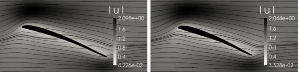
If a is parallel to the direction of the flow, then (1.4) represents the drag of the object B. If a is perpendicular to the direction of the flow, then (1.4) represents the lift of the object.

In the work at hand we propose an approach on how to deal with boundary objective functionals in the phase field setting. To be precise, we aim to minimize an appropriate phase field approximation of the functional (1.1), and also the functional (1.4), which can be considered as one of the most important objectives in shape optimization in fluids.

The fluid is assumed to be an incompressible, Newtonian fluid described by the stationary Navier–Stokes equations (1.2).

For this purpose, we first discuss how we model the integral over the free boundary Γ if it is replaced by a diffuse interface and how the normalν can be defined in this setting, see Section 3. Afterwards, we analyze the phase field problem for both (1.1) and (1.4) and discuss the existence of a minimizer and optimality conditions, see Section 4. In Section 5, we focus on the hydrodynamic force functional (1.4) and the corresponding phase field problem is then related to the sharp interface free boundary problem with a perimeter regularization by the method of matched formal asymptotic expansions. We find that the formal sharp interface limit of the optimality system gives the same results as can be found in the shape sensitivity literature.

We then solve the phase field problem numerically, see Section 6. For this purpose, we derive a gradient flow equation for the reduced objective functional and arrive in a Cahn–Hilliard type system. After time discretization, this system is treated in every time step by a Newton method. We numerically solve shape optimization problems involving drag and the lift-to-drag ratio.

2 Notation and problem formulation

Let us assume that Ω⊂R^d, d∈ {2,3}, is a fixed domain with Lipschitz boundary. Inside this fixed domain Ω we may have certain parts filled with fluid, denoted by E, and the complementB∶=Ω∖Eis some non-permeable medium. In the following we will denote by ν the outer unit normal ofB, i.e., the inner unit normal of the fluid region. The aim is to minimize the functional, given by (1.1), where Γ∶=∂B∩Ω, subject to the Navier–Stokes equations (1.2). We additionally impose a volume constraint on the amount of fluid. For this purpose we chooseβ∈ (−1,1)and only use fluid regionsE⊂Ω fulfilling the constraint

∣E∣ = ^(β+1)

2 ∣Ω∣.

We prescribe some inflow or outflow regions on the boundary of Ω and choose for this purpose g ∈H¹²(∂Ω) such that ∫_∂Ωg⋅ν_∂Ω dH^d−1 =0. Additionally, we may have some body forcef ∈L²(Ω) acting on the design domain. Note that throughout this paper we denoteR^d-valued functions and spaces consisting of R^d-valued functions in boldface.

As already mentioned in the introduction, problems like this are generally not well- posed in the sense that the existence of a minimizer can not be guaranteed. Hence, we use an additional perimeter regularization. For this purpose, we add a multiple of the perimeter of the obstacle to the cost functional (1.1). In order to properly formulate the resulting problem we introduce a design function ϕ ∶Ω→ {±1}, where {ϕ= 1} =E describes the fluid region and {ϕ= −1} = B is its complement. The volume constraint reads in this setting as∫_Ωϕdx =β∣Ω∣.

The design functions are chosen to be functions of bounded variation, such that the fluid region has finite perimeter, i.e., ϕ ∈ BV(Ω,{±1}). We shall write P_Ω(E) for the perimeter of some set of bounded variation E ⊆ Ω in Ω. Besides, if ϕ is a function of bounded variation, its distributional derivative Dϕ is a finite Radon measure and we can define the total variation by∣Dϕ∣ (Ω). Forϕ∈BV(Ω,{±1}), it holds that

∣Dϕ∣ (Ω) =2P_Ω({ϕ=1}). (2.1)

For a more detailed introduction to the theory of sets of finite perimeter and functions of bounded variation we refer to [11, 17]. We hence arrive in the following space of admissible design functions:

Φ⁰_ad∶= {ϕ∈BV(Ω,{±1}) ∣ ∫

Ωϕdx =β∣Ω∣}. (2.2) Let γ > 0 denote the weighting factor for the perimeter regularization. Then, we arrive at the following shape optimization problem for the functional (1.1) with additional perimeter regularization:

(ϕ,u,pmin)J₀(ϕ,u, p) ∶= ∫

Ω

1

2h(x,∇u, p,ν_ϕ)d∣Dϕ∣ +γ

2∣Dϕ∣ (Ω), (2.3)

subject toϕ∈Φ⁰_ad and(u, p) ∈H¹(E) ×L²(E) fulfilling

−µ∆u+ (u⋅ ∇)u+ ∇p=f inE= {ϕ=1}, (2.4a)

divu=0 in E, (2.4b)

u=g on∂Ω∩∂E, (2.4c)

u=0 on Γ=Ω∩∂E. (2.4d)

Here, we used the relation (2.1) to replace the perimeter of E with ¹₂∣Dϕ∣ (Ω). Fur- thermore, by the polar decomposition

Dϕ=ν_ϕ∣Dϕ∣ forϕ∈BV(Ω,{±1}), (2.5)

of the Radon measure Dϕ into a positive measure ∣Dϕ∣ and a S^d−1-valued function νϕ ∈ L¹(Ω,∣Dϕ∣)^d, see for instance [1, Corollary 1.29], we replace the product of the normal and the Hausdorff measure in (1.4) by ¹₂νϕd∣Dϕ∣. In particular,νϕ can be considered as a generalised unit normal on∂E.

We remark that the shape optimization problem (2.3) for the hydrodynamic force component (1.3) have been studied extensively in the literature. In the work of [2], the boundary integral (1.4) is transformed into a volume integral. This is also done in [7, 25], but in the latter, the compressible Navier–Stokes equations are considered. We also mention [21], which utilises the approach of Borrvall and Petersson [4] and the volume integral formulation. The shape derivatives for general volume and boundary objective functionals in Navier–Stokes flow have been derived in [26]. Finally, we mention the work of [3], which bears the most similarity to our set-up. Under the assumption that the set E= {ϕ=1} is C² and that there is a unique, sufficiently regular solution u to (1.2), the analysis of [3] obtained, via the speed method, that the shape derivative of

J(E) = ∫

Γa⋅ (µ(∇u+ (∇u)^T) −pI)νdH^d−1

with respect to vector fieldV is given by (see [3, Theorem 4, Equation 39])¹ DJ(E)[V] = ∫

Γ⟨V(0),ν⟩(f ⋅a+µ∂_νq⋅∂_νu)dH^d−1, (2.6)

1We remark that in [3], the normalnis pointing from the fluid domain to the obstacle, i.e., in comparison with our set-up,n= −ν.

whereq is the solution to the adjoint system (see [3, Equation 33.2]):

−µ∆q+ (∇u)^Tq− (u⋅ ∇)q+ ∇π=0 in E, (2.7a)

divq=0 in E, (2.7b)

q=aon Γ, (2.7c)

q=0 on ∂Ω∩∂E. (2.7d)

Here, we denote the normal derivative of a scalarα and of a vectorβ as

∂να∶= ∇α⋅ν, ∂νβ∶= (∇β)ν. (2.8) We note that asusatisfies the no-slip boundary condition (2.4d),u has no tangential components on Ω∩∂E. Thus, we obtain

∇u=∂_νu⊗ν on Γ=Ω∩∂E. (2.9)

Using the divergence free condition (2.4b), and the no-slip condition (2.4d), we obtain on Γ:

0= divu=tr(∇u) =

d

∑

i=1

∂νuiνi=∂νu⋅ν Ô⇒ (∇u)^Tν= (∂νu⋅ν)ν =0, (2.10) which in turn implies that

J(E) = ∫

Γa⋅ (σν)dH^d−1 = ∫

Γa⋅ (µ∇u−pI)νdH^d−1. (2.11) This is similar to the setting of [26, Remark 12] and by following the computations in [26]

one obtains (2.7) as the adjoint system and the shape derivative of (2.11) for aC² domain in the direction ofV is ²

DJ(E)[V] = ∫

Γ

⟨V(0),ν⟩ (−µ∂ν(∂νu) ⋅a+∂νp(a⋅ν) +µ∂νq⋅∂νu)dH^d−1

− ∫Γ

⟨V(0),ν⟩divΓ(µ(∇u)^Ta−pa)dH^d−1,

(2.12)

where div_Γdenotes the surface divergence. We introduce the surface gradient off on Γ by

∇_Γf with components(D_kf)_1≤k≤d, and with this definition we obtain div_Γv= ∑^d_k=1D_kv_k for a vector fieldv. Moreover, in components, we have

∂_ν(∂_νu) ⋅a=

d

∑

i,j,k=1

ν_i∂_i(ν_j∂_ju_k)a_k.

Remark 2.1. In [26, Remark 12], the term µ∂_ν(∂_νu) ⋅a appearing on the right hand side of (2.12) is originally given as ∑^d_i,j,k=1νi ∂²uk

∂xi∂xjνjak. This is related to ∂ν(∂νu) ⋅a by the formula

d

∑

i,j,k=1

νi

∂²uk

∂x_i∂x_jνjak=∂ν(∂νu) ⋅a−

d

∑

i,j,k=1

νi∂iν˜j∂jukak, (2.13) whereν˜= (ν˜j)_1≤j≤ddenotes an extension ofν off the boundaryΓto a neighbourhoodU ⊃Γ with∣ν˜∣ =1 near Γ and ν˜∣_Γ=ν.

2We remark that in [26, Remark 12] the term divΓ(µ(∇u)a) appears instead of divΓ(µ(∇u)^Ta), which we believe is a typo.

By (2.9), we see that ∂juk=∂νukνj on Γ, and so

d

∑

i,j,k=1

ν_i∂_iν˜_j∂_ju_ka_k=

d

∑

i,j,k=1

ν_i∂_iν˜_jν_j∂_νu_ka_k=

d

∑

i,j,k=1 1

2ν_i∂_i(∣˜ν_j∣²)∂_νu_ka_k=0. (2.14) Thus, the last term in (2.13) is zero and we have the relation

d

∑

i,j,k=1

ν_i ∂²u_k

∂xi∂xj

ν_ja_k=∂_ν(∂_νu) ⋅a, (2.15) whenu=0 onΓ.

Based on Remark 2.1, if (u, p) are sufficiently regular, then a short computation in- volving (2.15) shows that on Γ,

−µdivΓ((∇u)^Ta) −µ∂ν(∂νu) ⋅a+∂νp(a⋅ν) + divΓ(pa)

= −µ

d

∑

i=1

D_i(∂iuj)aj−µ

d

∑

i,j,k=1

νi∂_k(∂iuj)ν_kaj+ ∇p⋅a

= −µ∆u⋅a+ ∇p⋅a=f⋅a+ (u⋅ ∇)u⋅a=f ⋅a,

where we have used the no-slip condition (2.4d), and hence (2.12) is equivalent to (2.6).

3 Derivation of the phase field formulation

The problem derived in the previous section has several drawbacks. First, it is not clear if this is well-posed, i.e., if for every ϕ ∈ Φ⁰_ad there is a solution of the state equations (2.4) and if there exists a minimizer (ϕ,u, p) of the overall problem (2.3)-(2.4). Second, optimizing in the space BV(Ω) is not very practical. Deriving optimality conditions is not easy and it is not clear how to perform numerical simulations on this problem. Hence, we now want to approximate the complex shape optimization problem (2.3)-(2.4) by a problem that can be treated by well-known approaches. To this end we introduce a diffuse interface version of the free boundary problem by using a phase field approach.

3.1 The state equations in the phase field setting

In this setting, the design variableϕ∶Ω→Ris now allowed to have values in R, instead of only the two discrete values±1, and inherits H¹(Ω) regularity. In addition to the two phases{ϕ=1} (fluid region E) and{ϕ= −1} (solid region B), we also have an interfacial region{−1<ϕ<1}which is related to a small parameterε>0. By [22], we know that the Ginzburg–Landau energy

E_ε∶H¹(Ω) →R, E_ε(ϕ) ∶= ∫

Ω

ε

2∣∇ϕ∣² dx + 1

εψ(ϕ)dx (3.1)

approximatesϕ↦c₀∣Dϕ∣ (Ω) =2c₀P_Ω({ϕ=1}) in the sense of Γ-convergence. Here, c0∶=1

2∫

1

−1

√

2ψ(s)ds (3.2)

andψ∶R→Ris a potential with two equal minima at±1, and in this paper we focus on an arbitrary double-well potential satisfying the assumption below:

Assumption 3.1. Let ψ ∈ C^1,1(R) be a non-negative function such that ψ(s) = 0 if and only if s ∈ {±1}, and the following growth condition is fulfilled for some constants c₁, c₂, t₀>0 and k≥2:

c1t^k≤ψ(t) ≤c2t^k ∀t≥t0.

Additionally, we use the so-called porous medium approach for the state equations, see also [14, 15]. This means that, we relax the non-permeability of the solid region B outside the fluid by placing a porous medium of small permeability(αε)⁻¹≪1 outside the fluid regionE. In the interfacial region{−1<ϕ<1} we interpolate between the equations describing the flow through the porous medium and the stationary Navier–Stokes equations by using an interpolation functionαε satisfying the following assumption:

Assumption 3.2. We assume that αε∈C^1,1(R)is non-negative, withαε(1) =0,αε(−1) = αε>0, and there existsa, s_b∈Rwith sa≤ −1 and s_b≥1 such that

αε(s) =αε(sa) for s≤sa,

αε(s) =αε(sb) for s≥sb. (3.3) Moreover, we assume that the inverse permeability vanishes as ε↘0, i.e., limε↘0αε= ∞.

In particular, we have that

0≤αε(s) ≤ sup

t∈[sa,sb]αε(t) < ∞ ∀s∈R,

i.e.,α_ε∈L^∞(R). The resulting state equations for the phase field problem are then given in the strong form by the following system:

α_ε(ϕ)u−µ∆u+ (u⋅ ∇)u+ ∇p=f in Ω, (3.4a)

divu=0 in Ω, (3.4b)

u=g on ∂Ω. (3.4c)

Later we add ∫_Ω¹₂α_ε(ϕ) ∣u∣² dx to the objective functional and this ensures that in the limitε↘ 0, the velocity u vanishes outside the fluid region, and hence the medium can really be considered as non-permeable again.

In the following, we will use the following function spaces:

H_0,σ¹ (Ω) ∶= {v∈H₀¹(Ω) ∣ divv=0}, H_g,σ¹ (Ω) ∶= {v∈H¹(Ω) ∣v∣_∂Ω=g, divv=0}, and for the pressure we use the space L²₀(Ω) ∶= {p∈L²(Ω) ∣ ∫_Ωpdx =0}. The function space of admissible design functions for the phase field optimization problem will be given correspondingly to (2.2) as

Φ_ad∶= {ϕ∈H¹(Ω) ∣ ∫

Ωϕdx =β∣Ω∣}. 3.2 The cost functional in the phase field setting

We are now left to transfer the boundary integral in (2.3) to the diffuse interface setting where the free boundary Γ is replaced by an interfacial region. To this end, we apply a result of [22] and approximate the perimeter regularization term with _2c¹

0E_ε(ϕ). Mean- while, keeping in mind the polar decomposition (2.5) and the relation (2.1), we consider

the vector-valued measure with density ¹₂∇ϕas an approximation to νdH^d−1. Thus, we may approximate (2.3) with

∫Ω

1

2h(x,∇u, p,∇ϕ)dx+ γ

2c₀E_ε(ϕ).

Alternatively, we may appeal to the property of equipartition for the Ginzburg–Landau energy, i.e., it holds asymptotically that (see for instance, (5.29) in Section 5, or [9, Section 5.1]):

∫Ω

∣1

εψ(ϕε) −ε

2∣∇ϕε∣²∣dx ∼0 as ε↘0.

Hence, together with (2.1), and the fact that Γ-limit ofE_ε(ϕ)is the functionalc₀∣Dϕ∣ (Ω), defined for functions with values in{±1}, and +∞ otherwise, we have loosely speaking

2c0H^d−1⌞Γ∼c0∣Dϕ∣ ∼ ε

2∣∇ϕ∣²+1

εψ(ϕ) ∼ 2

εψ(ϕ), (3.5) where ₂^ε∣∇ϕ∣²+¹

εψ(ϕ)and ²_εψ(ϕ)are interpreted as measures on Ω, by using their values as densities. Here, we have identified Γ=∂{ϕ=1} ∩Ω with its reduced boundary, then it holds that ¹₂∣Dϕ∣ = ∣Dχ_{ϕ=1}∣ = H^d−1⌞Γ, see for instance [1, Theorem 3.59].

The generalised unit normal ν can be approximated by _∣∇^∇ϕ_ϕ∣. To rewrite this into a more convenient form, which is in particular differentiable with respect to ϕ, we use equipartition of energy and replace∣∇ϕ∣by ¹_ε

√

2ψ(ϕ), and obtain the approximation c0νdH^d−1∼ε ∇ϕ

√ 2ψ(ϕ)

1

εψ(ϕ)dx =

√ ψ(ϕ)

2 ∇ϕdx. (3.6)

Hence, we may also approximate (2.3) with 1

c0 ∫

Ω

√

ψ(ϕ)

2 h(x,∇u, p,∇ϕ)dx + γ 2c0

E_ε(ϕ), (3.7)

when we extendh(x,∇u, p,⋅) from unit vectors to all of Rⁿ such that h is positively one homogeneous with respect to its last variable. This allows us to extract the factor

√

ψ(ϕ) 2 . We note that in the bulk regions{ϕ= ±1}, we haveψ(ϕ) =0 and hence the functional (3.7) is not differentiable with respect to ϕ. Hence, we add a small constant δε to ψ in order to haveψ(s) +δ_ε>0 for alls∈R. However, we neglect the addition of this constant for the Ginzburg–Landau regularizationE_ε(ϕ) in the objective functional because adding a constant to the cost functional will not change the optimization problem.

In fact, for the analysis of the phase field problem, it is only important that δ_ε>0. In Section 5 where we perform a formal asymptotic analysis, we will require limε↘0δε=0 at a superlinear rate (see Remark 5.1).

3.3 Optimization problem in the phase field setting

Combining the above ideas, we arrive in the following phase field approximation:

(ϕ,u,pmin)J_ε^h(ϕ,u, p) ∶= ∫

Ω

1

2αε(ϕ) ∣u∣²+ 1 2c0

(ε

2∣∇ϕ∣²+1

εψ(ϕ))dx + ∫ΩM(ϕ)h(x,∇u, p,∇ϕ)dx,

(3.8)

subject toϕ∈Φad and(u, p) ∈H_g,σ¹ (Ω) ×L²₀(Ω) fulfilling

∫Ωα_ε(ϕ)u⋅v+µ∇u⋅ ∇v+ (u⋅ ∇)u⋅v−pdivvdx = ∫

Ωf ⋅vdx ∀v∈H₀¹(Ω). (3.9) Notice, that (3.9) is a weak formulation of the state equations (3.4). Moreover, based on the discussions in Section 3.2, the functionM(ϕ)can be chosen to be

M(ϕ) = 1

2 orM(ϕ) = 1 c0

√

ψ(ϕ)+δε

2 . (3.10)

The phase field approximation for the shape optimization problem with the hydrody- namic force (1.3) is obtained from (3.8) by substituting

h(x,∇u, p,∇ϕ) = ∇ϕ⋅ (µ(∇u+ (∇u)^T) −pI)a.

I.e.,

(ϕ,u,pmin)Jε(ϕ,u, p) ∶= ∫

Ω

1

2αε(ϕ) ∣u∣²+ 1 2c₀(ε

2∣∇ϕ∣²+1

εψ(ϕ))dx + ∫ΩM(ϕ)∇ϕ⋅ (µ(∇u+ (∇u)^T) −pI)adx,

(3.11)

subject toϕ∈Φ_ad and(u, p) ∈H_g,σ¹ (Ω) ×L²₀(Ω) fulfilling (3.9).

3.4 Possible modifications 3.4.1 Double obstacle potential

We could also use a double obstacle potentialψ∶R→R∪ {+∞}instead of the double-well potential in Assumption 3.1, i.e.,

ψ(ϕ) =

⎧⎪

⎪

⎨

⎪⎪

⎩

1

2(1−ϕ²) ifϕ∈ [−1,1],

+∞ if ∣ϕ∣ >1. (3.12)

Then, one has to treat the constraint ∣ϕ∣ ≤ 1 a.e. in the necessary optimality system either by writing the gradient equation in form of a variational inequality or by includ- ing additional Lagrange parameters. Numerical simulations could be implemented by a Moreau-Yosida relaxation as in [15]. A Moreau-Yosida relaxation also leads to a differ- entiable double well potential, and here we restrict ourselves to a differentiable potential where both settings can then be included in the above mentioned way.

3.4.2 Inequality constraint for fluid volume

Another possible modification of the problem setting would be to replace the equality con- straint∫_Ωϕdx =β∣Ω∣by an inequality constraint∫_Ωϕdx ≤β∣Ω∣. This would make sense in certain settings, if a maximal amount of fluid that can be used during the optimization process is prescribed and not the exact volume fraction. This would not change anything in the analysis, only that the Lagrange multiplier for this constraint would have a sign and an additional complementarity constraint appears in the optimality system.

3.4.3 Objective functionals with no dependency on the unit normal

We may also consider objective functionals with no dependence on the normal, i.e., the boundary objective functional (2.3) takes the form

∫Γk(x,∇u, p)dH^d−1. (3.13) An example of (3.13) is the best approximation to a target surface pressure distribution in the sense of least squares:

k(x,∇u, p) = 1

2∣p−p_d∣²,

where p_d denotes the target surface pressure distribution. Then, using (3.5), we deduce that the phase field approximation of (3.13) is given by

1 c₀∫

Ω

1

εψ(ϕ)k(x,∇u, p)dx.

If k(⋅,⋅,⋅) satisfies similar assumptions to Assumptions 4.1 and 4.2 (see below), one can adapt the proofs of Theorems 4.6 and 4.10 to obtain existence of a minimiser and the corresponding first order necessary optimality conditions.

4 Analysis of the phase field problem

In this section we want to analyze the phase field problem (3.8)-(3.9) derived in the previous section as a diffuse interface approximation of the shape optimization problem of minimizing (1.1) for a Navier–Stokes flow. For this purpose, we introduce some notation for the nonlinearity in the stationary Navier–Stokes equations. We define the trilinear form

b∶H¹(Ω) ×H¹(Ω) ×H¹(Ω) →R, b(u,v,w) ∶= ∫

Ω

(u⋅ ∇)v⋅wdx =

d

∑

i,j=1

∫Ωu_i∂_iv_jw_jdx. We directly obtain the following properties:

Lemma 4.1. The form b is well-defined and continuous in the space H¹(Ω) ×H¹(Ω) × H₀¹(Ω). Moreover we have:

∣b(u,v,w)∣ ≤K_Ω∥∇u∥_L2(Ω)∥∇v∥_L2(Ω)∥∇w∥_L2(Ω) ∀u,w∈H₀¹(Ω),v∈H¹(Ω), (4.1) with

K_Ω=

⎧⎪

⎪

⎨

⎪⎪

⎩

1

2∣Ω∣^1/2 if d=2,

2√ 2

3 ∣Ω∣^1/6 if d=3. (4.2)

Additionally, the following properties are satisfied:

b(u,v,v) =0 ∀u∈H¹(Ω),divu=0, v∈H₀¹(Ω), (4.3) b(u,v,w) = −b(u,w,v) ∀u∈H¹(Ω),divu=0, v,w∈H₀¹(Ω). (4.4)

Proof. The stated continuity and estimate (4.1) can be found in [13, Lemma IX.1.1] and (4.3)-(4.4) are considered in [13, Lemma IX.2.1].

Besides, we have the following important continuity property:

Lemma 4.2. Let (un)_n∈N,(vn)_n∈N,(wn)_n∈N⊂H¹(Ω), u,v,w∈H¹(Ω) be such thatun⇀ u, vn⇀v and wn⇀w in H¹(Ω) where vn∣_∂Ω=v∣_∂Ω for alln∈N. Then

nlim→∞b(un,vn,w˜) =b(u,v,w˜) ∀w˜ ∈H¹(Ω). (4.5) Moreover, one can show that

H¹(Ω) ×H¹(Ω) ∋ (u,v) ↦b(u,⋅,v) ∈H⁻¹(Ω) (4.6) is strongly continuous, and thus

n→∞lim b(un,vn,wn) =b(u,v,w). (4.7) Proof. We apply the idea of [32, Lemma 72.5] and make in particular use of the compact embeddingH¹(Ω) ↪L³(Ω) and the continuous embeddingH¹(Ω) ↪L⁶(Ω). The strong continuity of (4.6) follows from [32, Lemma 72.5]. In addition, from the boundedness of the sequences(u_n)_n∈N,(v_n)_n∈N,(w_n)_n∈N, and (4.6), we have

∣b(u_n,v_n,w_n) −b(u,v,w)∣

= ∣b(un−u,vn,wn)∣ + ∣b(u,vn,wn−w)∣ + ∣b(u,vn−v,w)∣

≤ ∥un−u∥_L3(Ω)

´¹¹¹¹¹¹¹¹¹¹¹¹¹¹¹¹¹¹¹¹¹¹¹¹¹¹¹¹¹¹¹¹¹¹¹¸¹¹¹¹¹¹¹¹¹¹¹¹¹¹¹¹¹¹¹¹¹¹¹¹¹¹¹¹¹¹¹¹¹¹¹¶

n→∞

ÐÐÐ→0

∥∇vn∥_L2(Ω)∥wn∥_L6(Ω)

´¹¹¹¹¹¹¹¹¹¹¹¹¹¹¹¹¹¹¹¹¹¹¹¹¹¹¹¹¹¹¹¹¹¹¹¹¹¹¹¹¹¹¹¹¹¹¹¹¹¹¹¹¹¹¹¹¹¹¹¹¹¹¹¹¹¹¸¹¹¹¹¹¹¹¹¹¹¹¹¹¹¹¹¹¹¹¹¹¹¹¹¹¹¹¹¹¹¹¹¹¹¹¹¹¹¹¹¹¹¹¹¹¹¹¹¹¹¹¹¹¹¹¹¹¹¹¹¹¹¹¹¹¹¶

≤C

+ ∥u∥_L6(Ω)∥∇vn∥_L2(Ω)

´¹¹¹¹¹¹¹¹¹¹¹¹¹¹¹¹¹¹¹¹¹¹¹¹¹¹¹¹¹¹¹¹¹¹¹¹¹¹¹¹¹¹¹¹¹¹¹¹¹¹¹¹¹¹¹¹¹¹¹¹¸¹¹¹¹¹¹¹¹¹¹¹¹¹¹¹¹¹¹¹¹¹¹¹¹¹¹¹¹¹¹¹¹¹¹¹¹¹¹¹¹¹¹¹¹¹¹¹¹¹¹¹¹¹¹¹¹¹¹¹¹¶

≤C

∥wn−w∥_L3(Ω)

´¹¹¹¹¹¹¹¹¹¹¹¹¹¹¹¹¹¹¹¹¹¹¹¹¹¹¹¹¹¹¹¹¹¹¹¹¹¹¸¹¹¹¹¹¹¹¹¹¹¹¹¹¹¹¹¹¹¹¹¹¹¹¹¹¹¹¹¹¹¹¹¹¹¹¹¹¹¶

n→∞

ÐÐÐ→0

+ ∣b(u,v_n−v,w)∣

´¹¹¹¹¹¹¹¹¹¹¹¹¹¹¹¹¹¹¹¹¹¹¹¹¹¹¹¹¹¹¹¹¹¹¹¹¹¹¹¹¹¹¸¹¹¹¹¹¹¹¹¹¹¹¹¹¹¹¹¹¹¹¹¹¹¹¹¹¹¹¹¹¹¹¹¹¹¹¹¹¹¹¹¹¹¹¶

n→∞

ÐÐÐ→0 by (4.6)

.

4.1 Existence results

In this section, we want to analyze the solvability of the state equations (3.9). Afterwards, we will show existence of a minimizer for the overall optimization problem (3.8)-(3.9).

Lemma 4.3. Let Assumption 3.2 hold. Then, for every ϕ∈ L¹(Ω) there exists at least one pair (u, p) ∈H_g,σ¹ (Ω) ×L²₀(Ω) such that the state equations (3.4) are fulfilled in the sense of (3.9). This solution (u, p) fulfils the estimate

∥u∥_H1(Ω)+ ∥p∥_L2(Ω)≤C(µ, αε,f,g,Ω), (4.8) with a constant C=C(µ, α_ε,f,g,Ω) independent of ϕ.

Proof. We refer to [14, Lemma 4], where the existence and uniqueness statements for the velocity field u are discussed. We point out, that the restriction to functions ϕ∈L¹(Ω) with∣ϕ∣ ≤1 a.e. in Ω used in [14] is only necessary because the functionαε in [14] is only defined on the interval[−1,1]. But of course, the same arguments apply to our case where αε is bounded andϕ∈L¹(Ω).

Now for every ϕ∈L¹(Ω)and u∈H_g,σ¹ (Ω) fulfilling

∫Ωαε(ϕ)u⋅v+µ∇u⋅ ∇v+ (u⋅ ∇)u⋅vdx = ∫

Ωf⋅vdx ∀v∈H_0,σ¹ (Ω), we find by [27, Lemma II.2.1.1] a uniquep∈L²₀(Ω) such that (3.9) together with

∥p∥_L2(Ω)≤C(Ω)∥α_ε(ϕ)u−µ∆u+ (u⋅ ∇)u−f∥_H−1(Ω)

is fulfilled. Combining this with the previous statements we can conclude the lemma.

This motivates the definition of a set-valued solution operator

Sε(ϕ) ∶= {(u, p) ∈H_g,σ¹ (Ω) ×L²₀(Ω) ∣ (u, p)fulfil (3.9)}forϕ∈L¹(Ω). (4.9) Remark 4.1. If there is some u∈Sε(ϕ) with ∥∇u∥_L2(Ω)< ^µ

KΩ, where K_Ω is defined in (4.2). Then Sε(ϕ) = {(u, p)}. I.e., there is exactly one solution of (3.9)corresponding to ϕ(see for instance [18, Lemma 11.5] or [14, Lemma 5]).

Moreover, we show a certain continuity property of the solution operator:

Lemma 4.4. Under Assumption 3.2, assume (ϕ_k)_k∈N⊂L¹(Ω) converges strongly to ϕ∈ L¹(Ω) in the L¹-norm and (u_k, p_k)_k∈N ⊂ H¹(Ω) ×L²(Ω) are given such that (u_k, p_k) ∈ Sε(ϕk) for allk∈N. Then there is a subsequence, which will be denoted by the same, such that(u_k, p_k)_k∈N converges strongly in H¹(Ω) ×L²(Ω) to some element (u, p) ∈Sε(ϕ). Proof. Let(ϕ_k)_k∈N and (u_k, p_k)_k∈N be chosen as in the statement. By passing to another subsequence, denoted the same, we can without loss of generality assume that ϕ_k → ϕ almost everywhere. Invoking (4.8), we obtain a uniform bound on (uk, pk) in H¹(Ω) × L²(Ω)because(u_k, p_k) ∈Sε(ϕ_k). And so there is a subsequence, which will be denoted by the same, such thatu_k converges weakly in H¹(Ω) and strongly in L²(Ω) to some limit elementu∈H_g,σ¹ (Ω) andpk converges weakly inL²(Ω)to some limit element p∈L²₀(Ω).

We now aim to show that F_k∶H_g,σ¹ (Ω) →R, F_k(v) ∶= ∫

Ω

1

2α_ε(ϕ_k) ∣v∣²+µ

2∣∇v∣²+ (u_k⋅ ∇)u_k⋅v−f⋅vdx, Γ-converges inH_g,σ¹ (Ω) equipped with the weak topology to

F_∞∶H_g,σ¹ (Ω) →R, F_∞(v) ∶= ∫

Ω

1

2α_ε(ϕ) ∣v∣²+µ

2∣∇v∣²+ (u⋅ ∇)u⋅v−f⋅vdx,

ask→ ∞. To see this we first notice that for any sequence(v_k)_k∈N⊆H_g,σ¹ (Ω)converging weakly inH¹(Ω) tov∈H_g,σ¹ (Ω), by Fatou’s lemma it holds that

∫Ωα_ε(ϕ) ∣v∣² dx ≤lim inf

k→∞ ∫

Ωα_ε(ϕ_k) ∣v_k∣² dx.

Applying the boundedness and continuity properties of the trilinear form b(⋅,⋅,⋅), see Lemma 4.1 and 4.2, we can deduce that lim_k→∞b(u_k,u_k,v_k) = b(u,u,v). As the re- maining terms ofFk are weakly lower semicontinuous in H¹(Ω) and independent of ϕk, we directly obtain

F_∞(v) ≤lim inf

k→∞ F_k(v_k).

Letv∈H_g,σ¹ (Ω) be chosen. We will show, that the constant sequence(v)_k∈N defines a recovery sequence. For this purpose, we notice that due to the boundedness and continuity ofα_ε, we have from Lebesgue’s dominated convergence theorem

k→∞lim ∫

Ωα_ε(ϕ_k) ∣v∣² dx = ∫

Ωα_ε(ϕ) ∣v∣² dx. (4.10)

Invoking (4.5) in Lemma 4.2, we deduce that

klim→∞b(uk,uk,v) =b(u,u,v),

and thus, we obtain that lim_k→∞F_k(v) =F_∞(v). This shows that the Γ-limit of (F_k)_k∈N inH_g,σ¹ (Ω) with respect to the weak topology equalsF_∞.

Now we notice, thatu_k is exactly the unique minimizer ofF_k inH_g,σ¹ (Ω), as it fulfils per definition the necessary and sufficient first order optimality conditions for the convex optimization problem min_u∈H¹

g,σ(Ω)F_k(u). Hence, the weakH¹(Ω)limit of(u_k)_k∈N, which isu∈H_g,σ¹ (Ω), is the unique solution of min_u∈H¹

g,σ(Ω)F_∞(u), thus it holds that

∫Ωα_ε(ϕ)u⋅v+µ∇u⋅ ∇v+ (u⋅ ∇)u⋅vdx = ∫

Ωf ⋅vdx ∀v∈H_0,σ¹ (Ω). (4.11) By [27, Lemma II.2.1.1] we can associate to (4.11) a unique ˜p∈L²₀(Ω) such that (3.9) is fulfilled, and hence ˜p=p. Altogether we have shown (u, p) ∈Sε(ϕ).

To show the strong convergence inH¹(Ω)×L²(Ω), we note that from the Γ-convergence of (F_k)_k∈N toF_∞ we obtain additionally that lim_k→∞F_k(u_k) =F_∞(u). Invoking Lemma 4.5 below we find

klim→∞∫

Ωα_ε(ϕ_k) ∣u_k∣² dx = ∫

Ωα_ε(ϕ) ∣u∣²dx. In addition, by means of (4.7) from Lemma 4.2 we have

klim→∞b(u_k,u_k,u_k) =b(u,u,u).

These two results allow us to deduce from the convergence of the minimal functional values of(F_k)_k∈Nthat lim_k→∞∫_Ω∣∇u_k∣² dx = ∫_Ω∣∇u∣² dx . Then, together withu_k⇀uinH¹(Ω) this yields that lim_k→∞∥u_k−u∥_H1(Ω)=0.

Subtracting the state equations (3.9) written for ϕ from the state equations (3.9) written forϕ_k, we find from Lemma 4.5 below that

∫Ω

(pk−p)divvdx = ∫

Ω

(αε(ϕk)uk−αε(ϕ)u) ⋅v+µ∇(uk−u) ⋅ ∇vdx +b(u_k,u_k,v) −b(u,u,v)

≤ ∥α_ε(ϕ_k)u_k−α_ε(ϕ)u∥_L2(Ω)

´¹¹¹¹¹¹¹¹¹¹¹¹¹¹¹¹¹¹¹¹¹¹¹¹¹¹¹¹¹¹¹¹¹¹¹¹¹¹¹¹¹¹¹¹¹¹¹¹¹¹¹¹¹¹¹¹¹¹¹¹¹¹¹¹¹¹¹¹¹¹¹¹¹¹¹¹¹¹¹¹¹¹¹¹¹¸¹¹¹¹¹¹¹¹¹¹¹¹¹¹¹¹¹¹¹¹¹¹¹¹¹¹¹¹¹¹¹¹¹¹¹¹¹¹¹¹¹¹¹¹¹¹¹¹¹¹¹¹¹¹¹¹¹¹¹¹¹¹¹¹¹¹¹¹¹¹¹¹¹¹¹¹¹¹¹¹¹¹¹¹¹¹¶

k→∞

ÐÐÐ→0

∥v∥_L2(Ω)+µ∥u_k−u∥_H1(Ω)

´¹¹¹¹¹¹¹¹¹¹¹¹¹¹¹¹¹¹¹¹¹¹¹¹¹¹¹¹¹¹¹¹¹¹¹¹¸¹¹¹¹¹¹¹¹¹¹¹¹¹¹¹¹¹¹¹¹¹¹¹¹¹¹¹¹¹¹¹¹¹¹¹¹¹¶

k→∞

ÐÐÐ→0

∥v∥_H1(Ω)

+ ∥b(u_k,u_k,⋅) −b(u,u,⋅)∥_H−1(Ω)

´¹¹¹¹¹¹¹¹¹¹¹¹¹¹¹¹¹¹¹¹¹¹¹¹¹¹¹¹¹¹¹¹¹¹¹¹¹¹¹¹¹¹¹¹¹¹¹¹¹¹¹¹¹¹¹¹¹¹¹¹¹¹¹¹¹¹¹¹¹¹¹¹¹¹¹¹¹¹¹¹¹¹¹¹¹¹¹¹¹¹¹¹¹¹¹¹¹¹¹¸¹¹¹¹¹¹¹¹¹¹¹¹¹¹¹¹¹¹¹¹¹¹¹¹¹¹¹¹¹¹¹¹¹¹¹¹¹¹¹¹¹¹¹¹¹¹¹¹¹¹¹¹¹¹¹¹¹¹¹¹¹¹¹¹¹¹¹¹¹¹¹¹¹¹¹¹¹¹¹¹¹¹¹¹¹¹¹¹¹¹¹¹¹¹¹¹¹¹¹¹¶

k→∞

ÐÐÐ→0

∥v∥_H1(Ω).

Thus lim_k→∞∥∇(p_k−p)∥_H−1(Ω)=0. Using now the pressure estimate, see for instance [27, Lemma II.1.5.4], we find

∥p_k−p∥_L2(Ω)≤c∥∇(p_k−p)∥_H−1(Ω) k→∞

ÐÐÐ→0.

Therefore, we deduce that(p_k)_k∈N converges strongly in L²(Ω) top.

In the previous proof we made use of the following lemma:

Lemma 4.5. Under Assumption 3.2, assume that for (ϕ_k)_k∈N⊂L¹(Ω),(u_k)_k∈N⊂L²(Ω) andϕ∈L¹(Ω), u∈L²(Ω),

klim→∞∥ϕ_k−ϕ∥_L1(Ω)=0, ϕ_k→ϕ a.e. and lim

k→∞∥u_k−u∥_L2(Ω)=0.

Then it holds that

klim→∞∫

Ωαε(ϕk) ∣uk∣² dx = ∫

Ωαε(ϕ) ∣u∣² dx and lim

k→∞∥αε(ϕk)uk−αε(ϕ)u∥_L2(Ω)=0.

Proof. Using the ideas of [18, Theorem 5.1] and [14, Theorem 1] we find that

∣∫Ωα_ε(ϕ_k) ∣u_k∣²−α_ε(ϕ) ∣u∣² dx∣ = ∫

Ωα_ε(ϕ_k) (∣u_k∣²− ∣u∣²)dx + ∫Ω

(αε(ϕk) −αε(ϕ)) ∣u∣² dx, and fromα_ε∈L^∞(R) we obtain

∫Ωα_ε(ϕ_k) (∣u_k∣²− ∣u∣²)dx ≤ ∥α_ε∥_L∞(R)∥u_k+u∥_L2(Ω)∥u_k−u∥_L2(Ω) k→∞

ÐÐÐ→0.

Moreover, the uniform bound onα_ε yields by Lebesgue’s dominated convergence theorem

klim→∞∫

Ω(α_ε(ϕ_k) −α_ε(ϕ)) ∣u∣² dx =0, which combined with the previous step yields the first assertion.

Using a similar idea we find

∥αε(ϕ_k)u_k−αε(ϕ)u∥_L2(Ω)≤ ∥αε(ϕ_k)(u_k−u)∥_L2(Ω)+ ∥(αε(ϕ_k) −αε(ϕ))u∥_L2(Ω)

≤ ∥αε∥_L∞(R)∥uk−u∥_L2(Ω)+ ∥(αε(ϕk) −αε(ϕ))u∥_L2(Ω) k→∞

ÐÐÐ→0, where we applied Lebesgue’s dominated convergence theorem in order to deduce from α_ε∈L^∞(R)that lim_k→∞∥(α_ε(ϕ_k) −α_ε(ϕ))u∥_L2(Ω)=0.

We make the following assumption regarding h:

Assumption 4.1. Let h∶Ω×R^d×d×R×R^d→Rbe a Carath´eodory function, which fulfils 1. h(⋅,A, s,w) ∶Ω→R is measurable for each w∈R^d, s∈R,A∈R^d×d, and

2. h(x,⋅,⋅,⋅) ∶R^d×d×R×R^d→Ris continuous for almost every x∈Ω.

Moreover, there exist non-negative functions a∈ L¹(Ω), b1, b2, b3 ∈ L^∞(Ω) such that for almost everyx∈Ωit holds

∣h(x,A, s,w)∣ ≤a(x) +b₁(x) ∣A∣²+b₂(x) ∣s∣²+b₃(x) ∣w∣², for allw∈R^d, s∈R,A∈R^d×d.

Furthermore, the functional H ∶H¹(Ω) ×L²(Ω) ×H¹(Ω) →R defined as H(u, p, ϕ) ∶= ∫

Ω

M(ϕ)h(x,∇u, p,∇ϕ)dx, satisfy the following properties

(i) H ∣_H1

g,σ(Ω)×L²₀(Ω)×Φad is bounded from below, and

(ii) for all ϕ_n⇀ϕin H¹(Ω), u_n→u in H¹(Ω), p_n→p in L²(Ω), it holds that H(u, p, ϕ) ≤lim inf

n→∞ H(un, pn, ϕn). We then obtain the following existence result for (3.8)-(3.9):

Theorem 4.6. Under Assumptions 3.1, 3.2 and 4.1, there exists at least one minimizer of the optimal control problem (3.8)-(3.9).

Proof. We may restrict ourselves to consideringϕ∈Φ_adwithϕ∈ [s_a, s_b]a.e. in Ω. In fact, we define as in [22, Proof of Proposition 1] for arbitraryϕ∈Φ_ad the truncated functions

˜

ϕ∶=max{sa,min{ϕ, sb}} and find E_ε(ϕ˜) ≤ E_ε(ϕ), where E_ε is defined in (3.1). Moreover, by (3.3), we haveαε(ϕ) =αε(ϕ˜) and hence alsoSε(ϕ) =Sε(ϕ˜). Therefore we obtain

J_ε^h(ϕ,˜ u, p) ≤J_ε^h(ϕ,u, p) for all (u, p) ∈Sε(ϕ) =Sε(ϕ˜). By Assumption 4.1, H ∣_H1

g,σ(Ω)×L²₀(Ω)×Φad is bounded below by a constant C₀, and so J_ε^h∶Φ_ad×H_g,σ¹ (Ω) ×L²₀(Ω)is bounded from below by a constantC₁. Thus, we can choose a minimizing sequence(ϕ_n,u_n, p_n)_n∈N⊂Φ_ad×H_g,σ¹ (Ω) ×L²₀(Ω)with(u_n, p_n) ∈S_ε(ϕ_n)for alln and

nlim→∞J_ε^h(ϕ_n,u_n, p_n) = inf

ϕ∈Φad,(u,p)∈Sε(ϕ)J_ε^h(ϕ,u, p) > −∞.

In particular, from the non-negativity of ψ and αε, we see that for ρ>0, there exists an N such thatn>N implies

C₀+ γε 2c0

∥∇ϕ_n∥_L2(Ω)≤J_ε^h(ϕ_n,u_n, p_n) ≤ inf

ϕ∈Φad,(u,p)∈Sε(ϕ)J_ε^h(ϕ,u, p) +ρ.

Thus, {∇ϕ_n}_n∈N is bounded uniformly in L²(Ω). Moreover, without loss of generality, we may assume that ϕ_n(x) ∈ [s_a, s_b] for a.e. x ∈Ω and every n∈N. And so, we deduce that{ϕn}_n∈N is bounded uniformly inH¹(Ω) ∩L^∞(Ω), and we may choose a subsequence (ϕ_nk)_k∈Nthat converges strongly inL²(Ω)and pointwise almost everywhere in Ω to some limit elementϕ∈Φ_ad.

Using Lemma 4.4 we can deduce that there is a subsequence of(un_k, pn_k)_k∈N, denoted by the same index, such that

klim→∞∥unk−u∥_H1(Ω)=0, lim

k→∞∥pnk−p∥_L2(Ω)=0, (4.12) and(u, p) ∈Sε(ϕ).

From Lemma 4.5 we deduce additionally that

klim→∞∫

Ωα_ε(ϕ_nk) ∣u_nk∣² dx = ∫

Ωα_ε(ϕ) ∣u∣² dx. (4.13) As sup_k∈N∥ψ(ϕ_nk)∥_L∞(Ω) < ∞ we can use Lebesgue’s dominated convergence theorem to deduce lim_k→∞∫_Ωψ(ϕ_nk)dx = ∫_Ωψ(ϕ)dx . Finally, the weak lower semicontinuity of H¹(Ω) ∋ϕ↦ ∫_Ω∣∇ϕ∣² dx yields

∫Ω

ε

2∣∇ϕ∣²+ 1

εψ(ϕ)dx ≤lim inf

k→∞ ∫

Ω

ε

2∣∇ϕ_nk∣²+ 1

εψ(ϕ_nk)dx. (4.14)