Sharp Interface Limit for a Stokes/ Cahn-Hilliard System

(1)

System

Dissertation

zur Erlangung des Doktorgrades der Naturwissenschaften (Dr. rer. nat.)

der Fakultät Mathematik der Universität Regensburg

vorgelegt von

Andreas Marquardt (geb. Schöttl)

aus Lichtenfels

im Jahr 2018

(2)

Promotionsgesuch eingereicht am:

Die Arbeit wurde angeleitet von: Prof. Dr. Helmut Abels Prüfungsausschuss:

Vorsitzender: Prof. Dr. Bernd Ammann Erst-Gutachter: Prof. Dr. Helmut Abels Zweit-Gutachter: Dr. Yuning Liu

weiterer Prüfer: Prof. Dr. Harald Garcke

Ersatzprüfer: Prof. Dr. Georg Dolzmann

(3)

(4)

Abstract

We rigorously show the sharp interface limit of a coupled Stokes/Cahn–Hilliard system in a two dimensional, bounded and smooth domain, i.e. we consider the limiting behavior of solutions when a parameter >0corresponding to the thickness of the diﬀuse interface tends to zero. We show that for suﬃciently short times the solutions to the Stokes/Cahn–Hilliard system converge to solutions of a sharp interface model, where the evolution of the interface is governed by a Mullins–Sekerka system with an additional convection term coupled to a two–phase stationary Stokes system with an extra contribution to the stress tensor, representing the capillary stress.

To show the sharp interface limit, we construct suitable approximate solutions to the Stokes/Cahn–Hilliard system, by devising an inductive scheme which allows for the construction of terms of arbitrarily high order in the formally matched asymptotic calculations.

As a novelty, we also introduce fractional order terms, which are of signiﬁcant importance.

In order to estimate the diﬀerence between the exact and the approximate solutions, we make use of modiﬁcations of spectral estimates shown in [24] for the linearized Cahn-Hilliard operator. The treatment of the involved coupling terms poses several complications, which have to be overcome by intricate analysis.

Wir führen einen rigorosen Beweis für einen scharfen Grenzschicht-Limes eines gekoppel- ten Stokes/Cahn–Hilliard Systems in einem zweidimensionalen, beschränkten und glatten Gebiet. Dazu betrachten wir das Verhalten von Lösungen, wenn ein Parameter > 0, welcher die Dicke der diﬀusen Grenzschichtregion beschreibt, gegen Null geht. Wir zeigen, dass Lösungen des Stokes/Cahn–Hilliard Systems für hinreichend kurze Zeiten gegen Lösun- gen eines scharfen Grenzschicht-Modells konvergieren, in welchem die Evolution der Gren- zschicht durch ein Mullins–Sekerka System mit zusätzlichem Konvektionsterm bestimmt wird, welches an ein Zwei-Phasen Stokes System gekoppelt ist, das einen zusätzlichen, Kap- illarkräfte repräsentierenden Term im Spannungstensor aufweist.

Um den scharfen Grenzschicht-Limes zu beweisen, konstruieren wir geeignete Approxima- tionslösungen des Stokes/Cahn-Hilliard Systems mit Hilfe eines induktiven Schemas, welches es uns erlaubt, Terme beliebig hoher Ordnung in den Rechnungen zur formalen asymptotis- chen Entwicklung zu konstruieren. Als Neuerung führen wir zusätzlich Terme gebrochener Ordnung ein, die sich im Verlauf der Arbeit als zentrales Element herausstellen. Um die Dif- ferenz zwischen den exakten und approximativen Lösungen abschätzen zu können, nutzen wir eine Modiﬁkation der Spektralabschätzung für den linearisierten Cahn–Hilliard Opera- tor, welche in [24] gezeigt wurde. Die Behandlung der vorkommenden Kopplungsterme wirft mehrere Schwierigkeiten auf, welche einer aufwendigen Analyse bedürfen.

(5)

(6)

1. Introduction

“According to Gibbs’ theory, capillary phenomena are present only if there is a discontinuity between the portions of ﬂuid that are face-to-face. [...] In contrast, the method that I propose to develop in the following pages is not a satisfactory treatment unless the density of the body varies continuously at and near its transition layer. It will not be without interest to show that the two apparently contradictory hypotheses lead to values of the same order of magnitude [...].”

–Van der Waals, [45]

Classically, the transition between two immiscible fluids was considered to be abrupt, in the sense of an appearance of a lower-dimensional surface separating the phases. Famous historical figures such as Young, Laplace and Gauß were advocating this point of view and developing the theory behind it, see [15, 46]. Considering the transitional layer to have zero thickness, it is reasonable to take into account geometric quantities such as curvature and physical properties such as surface tension. The behavior of a multiphase system is then governed by the intricate interactions between the bulk regions and the interface, mathemat- ically expressed as equations of motion, which hold in each fluid, complemented by boundary conditions at the (free) surface. Models incorporating these ideas – often calledsharp inter- face models – and the corresponding free-boundary problems have been widely studied and used to great success in describing a multitude of physical and biological phenomena. These range from the classical Stefan Problem, over image development in electrophotography, the theory of two-phase bio membranes, fluid flow through porous media, up to tumor growth, see [18, 50, 30, 17, 32] and the references therein.

However, fundamental problems arise in the analysis and numerical simulation of such problems, whenever the considered interfaces develop singularities. In fluid dynamics, topo- logical changes such as the pinch off of droplets or collisions are non-negligible features of many systems, having a significant impact on the flow.

Conversely,diffuse interface modelsturn out to provide a promising, alternative approach to describe such phenomena and overcome the associated difficulties. In these diffuse interface (orphase field)methods, a partial mixing of the two phases is taken into consideration, allowing for the quantities, which were localized to a surface in the free-boundary formulation, to be spread out throughout an interfacial region. To this end, an order parameter (poten- tially signifying concentration, density, velocity etc.) is introduced, which varies rapidly, but smoothly, throughout a thin interfacial layer, heuristically viewed to have a thickness pro- portional to a length scale parameter > 0. As emphasized by the introductory epigraph, these ideas go back to the writings of Van der Waals and Lord Rayleigh and have gained considerable traction with the works of Cahn and Hilliard, see [15, 45, 23] with regard to the historical sources and e.g. [39, 1, 2, 20] for more recent results.

Naturally, together with the appearance of a transitional layer of thickness corresponding to > 0 the question of the limit case → 0 arises. This so-called sharp interface limit is in fact a question about the connection of sharp and diﬀuse interface models. As phase ﬁeld approaches may also be used as a tool, alongside level set methods and parametric

(9)

techniques, to numerically solve free boundary problems and surface evolution equations (see also [27]), it is of paramount importance to know that they asymptotically approach the correct sharp interface models.

Concerning the flow of two macroscopically immiscible, viscous, incompressible Newtonian fluids with matched densities, a fundamental and broadly accepted diffuse interface model is the so-called model H, derived in [39, 36]. This model consists of a Navier-Stokes system coupled with the Cahn-Hilliard equation and is of the form

ρ∂_tv^ϵ+ρv^ϵ· ∇v^ϵ−div(2ν(c^ϵ)D_sv^ϵ) +∇p^ϵ=−div(∇c^ϵ⊗ ∇c^ϵ) inΩ_T, (1.1)

divv^ϵ= 0 inΩ_T, (1.2)

∂tc^ϵ+v^ϵ· ∇c^ϵ=m^ϵ∆µ^ϵ inΩT, (1.3) µ^ϵ=−∆c^ϵ+⁻¹f^′(c^ϵ) inΩ_T, (1.4) (v^ϵ, c^ϵ)|t=0= (v^ϵ₀, c^ϵ₀) inΩ. (1.5) Here T >0,Ω⊂Rⁿ,n∈N, is a bounded and smooth domain,ΩT = Ω×(0, T) and

(a⊗b)_i,j =a_ib_j (1.6)

for all i, j∈ {1, . . . , n} anda,b∈Rⁿ. v^ϵ and p^ϵ represent the mean velocity and pressure,

Dsv^ϵ = 1 2

∇v^ϵ+ (∇v^ϵ)^T

, (1.7)

c^ϵ is an order parameter representing the concentration difference of the fluids and µ^ϵ is the chemical potential of the mixture. Moreover, v^ϵ₀ and c^ϵ₀ are suitable initial values, ρ is the (supposedly constant) density of the fluids, ν is the viscosity of the mixture and m^ϵ >0 is a mobility coefficient related to the strength of the diffusion in the mixture. The function f :R → R is supposed to be a homogeneous free energy density of double-well shape, the exact specifications of which will be given later. This system is usually supplemented by a no-slip boundary condition forv^ϵ and Neumann boundary conditions for c^ϵ and µ^ϵ, i.e.

(v^ϵ,n∂Ω· ∇c^ϵ,n∂Ω· ∇µ^ϵ) = 0 on∂TΩ,

where∂_TΩ =∂Ω×(0, T) and n_∂Ω denotes the outer unit normal. To gain an inkling of the sharp interface limit of a system like (1.1)–(1.5) the so-called method of formally matched asymptotics has in recent years proven to be a very ﬂexible and accessible approach, see e.g.

[21, 33, 43]. The underlying idea of this method is to assume that the appearing variables may be expressed as power series or asymptotic expansions in , with diﬀerent expansions close to and away from the interface, which allows for the consideration of diﬀerent length scales.

Additionally, the expansions are supposed to satisfy certain matching-properties, providing a connection between the bulk and interfacial regions (for more detailed assumptions and explanations, see the introduction of Chapter 5).

In the case of (1.1)–(1.5) such formal calculations have been done in [4] and yield in the

(10)

case of a constant mobility m^ϵ=m0 >0the sharp interface system

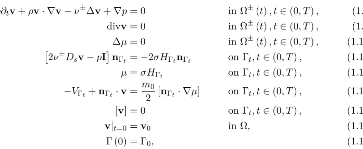
ρ∂tv+ρv· ∇v−ν^±∆v+∇p= 0 inΩ^±(t), t∈(0, T), (1.8) divv= 0 inΩ^±(t), t∈(0, T), (1.9)

∆µ= 0 inΩ^±(t), t∈(0, T), (1.10) 2ν^±D_sv−pI

n_Γ_t =−2σH_Γ_tn_Γ_t onΓ_t, t∈(0, T), (1.11) µ=σH_Γ_t onΓ_t, t∈(0, T), (1.12)

−V_Γ_t+n_Γ_t ·v= m₀

2 [n_Γ_t · ∇µ] onΓ_t, t∈(0, T), (1.13) [v] = 0 onΓt, t∈(0, T), (1.14)

v|t=0=v0 inΩ, (1.15)

Γ (0) = Γ₀, (1.16)

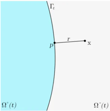
closed by suitable boundary conditions on∂Ω×(0, T). HereΩis the disjoint union ofΩ⁺(t), Ω⁻(t)andΓtfor everyt∈[0, T0], whereΓt=∂Ω⁺(t),nΓt is the exterior normal with respect toΩ⁻(t), andH_Γ_t and V_Γ_t denote the mean curvature and normal velocity of the interface Γt. Furthermore, we use the notations

[g] (p, t) := lim

h↘0(g(p+nΓt(p)h)−g(p−nΓt(p)h)) forp∈Γt, σ:= 1

2 ˆ1

−1

p2f(s)ds, (1.17)

and denote byΓ0 a given initial surface and byν^± the viscosity in the bulk phases.

Figure 1.1.: A schematic representation of the general situation.

The identities (1.8), (1.9) correspond to the conservation of linear momentum and mass in the ﬂuids, while (1.11) represents the jump in the stress tensor and (1.13) is a Stefan type

(11)

condition for the evolution of the interface. If m0 vanished, i.e. no diffusion of mass was taken into account, the latter would reduce to a pure transport equation. The system of equations (1.10), (1.12) and (1.13) (with v= 0) are also known as the Mullins–Sekerka flow and may be obtained as the H⁻¹ gradient flow of the area functional, see e.g. [34]. Hence, system (1.8)–(1.16) is commonly referred to as a Navier–Stokes/Mullins–Sekerka system.

Regarding the existence of solutions for (1.1)–(1.5) we refer to [2, 19]; short time existence of strong solutions of (1.8)–(1.16) was shown in [11] and existence of weak solutions for long times in [9]. Despite these analytic results and the formal findings for the sharp interface limit, there are only few attempts at rigorously showing the convergence of solutions of the diffuse interface system (1.1)–(1.5) to solutions of the sharp interface system (1.8)–(1.16) as → 0. This does not only hold true for the model H, but reflects the general situation in the theory of two-phase flows in fluid mechanics. One approach to rigorously proving sharp interface limits uses the notion of varifold solutions discussed in [25]; in the setting of two phase flows, such results for large times were shown in [9] for the model H and in [5] also for the more general situation of fluids with different densities. The pursued strategy in these works is to show (weak) compactness for the families of weak solutions to the corresponding diffuse interface system in suitable spaces, which then allows for the extraction of a convergent subsequence. It is then proven that the limit of such a subsequence is given by a varifold solution of the affiliated sharp interface system. The limitations of this technique are inherent to the underlying mathematical principles, as the notion of varifold solutions is rather weak and no convergence rates may be obtained from the compactness arguments.

Another approach is based on the works [42] and [14], where the method of formally matched asymptotics is used as a basis. It is assumed that both the considered diffuse and sharp interface model have smooth solutions in a short time interval (0, T); in the case of [14] these systems consist of the Cahn-Hilliard equation and the Mullins-Sekerka (or Hele- Shaw) system. Using matched asymptotic expansions, an explicit approximate solution to the diffuse interface system is constructed, usually consisting of significantly more terms than needed for an only formal investigation. The key element of the argumentation is then to show that the difference between the real solutions and the approximate solutions tends to 0 in suitable (strong) norms as → 0. As the detailed structure of the approximate solutions is known, it may then easily be verified that they in turn converge to solutions of the underlying sharp interface system, yielding a result for the sharp interface limit. This strategy has been successfully adapted to a lot of different problems over the years: in [26]

the mass conserving Allen-Cahn equation was connected to the volume preserving mean curvature flow, in [10] it was used to show the convergence of the Cahn–Larché system to a modified Hele–Shaw problem and in [22] several phase field models were considered. Most recently the approach has also been used to show the sharp interface limit for an Allen-Cahn system with 90^◦-contact angle, see [8].

However, in view of two-phase flow models in fluid mechanics and the arising difficulties therein, the first and so far only convergence result with convergence rates in strong norms is [6]. Considering a coupled Stokes/Allen-Cahn system in two dimensions, it is shown that smooth solutions of the diffuse interface system converge for short times to solutions of a sharp interface model, where the evolution of the free surface is governed by a convective mean curvature flow coupled to a two-phase Stokes system with a modified stress tensor, accounting for capillary forces. The Stokes/Allen-Cahn system is analyzed as it allows for the study of arising problems in the context of two phase flows within a simplified setting, neither having to take into account the instationary character and the nonlinearities of Navier-Stokes type equations, nor having to deal with a fourth order partial differential equation like the

(12)

Cahn-Hilliard equation and its more technically involved asymptotic expansion.

This contribution builds upon the ideas introduced in [6] and aims to establish the ﬁrst rigorous result in strong norms for a sharp interface limit of a two phase ﬂow model involving the Cahn-Hilliard equation with convergence rates. In doing so, we hope to build another cornerstone on the way to rigorously showing the sharp interface limit for model H.

More precisely we consider the Stokes/Cahn-Hilliard system

−∆v^ϵ+∇p^ϵ =µ^ϵ∇c^ϵ inΩ_T, (1.18)

divv^ϵ = 0 inΩT, (1.19)

∂tc^ϵ+v^ϵ· ∇c^ϵ = ∆µ^ϵ inΩT, (1.20)

µ^ϵ =−∆c^ϵ+1

f^′(c^ϵ) inΩ_T, (1.21)

c^ϵ|t=0 =c^ϵ₀ inΩ, (1.22)

(−2D_sv^ϵ+p^ϵI)·n_∂Ω =α₀v^ϵ on∂_TΩ, (1.23)

µ^ϵ = 0 on∂_TΩ, (1.24)

c^ϵ =−1 on∂_TΩ, (1.25)

where Ω ⊂R² is a domain with smooth boundary, α₀ >0 is ﬁxed and c^ϵ₀ is certain “well- chosen” initial data (see Theorem 4.1 for more details; we allow perturbations of some order ofaround a given value). Note that forψ∈C_0,σ^∞ (Ω) :=

n

ψ∈C₀^∞(Ω)²divψ= 0 o

we have by (1.21)

ˆ

Ω

µ^ϵ∇c^ϵ·ψdx= ˆ

Ω

−∆c^ϵ∇c^ϵ+1

∇(f(c^ϵ))

·ψdx=− ˆ

Ω

div(∇c^ϵ⊗ ∇c^ϵ)·ψdx,

where we used integration by parts and div(∇c^ϵ⊗ ∇c^ϵ)−¹₂∇ |∇c^ϵ|²=∇c^ϵ∆c^ϵin the second equality. Thus, in the case of a no-slip boundary condition forv^ϵ instead of (5.86), the right hand sides of (1.1) and (1.18) coincide in the weak formulation.

Existence of smooth solutions to (1.18)–(1.25) can be shown with similar methods as in [2], where the considered model is in fact way more complicated, as it involves the full Navier-Stokes equation. A word is in order about the unusual choice of boundary conditions (1.23)–(1.25). (1.23) can be thought of as a modified do-nothing boundary condition (−2Dsv^ϵ+p^ϵI)·n∂Ω = 0, which is equivalent to the case α0 = 0 or as an altered Navier boundary condition. Physically, it would be sensible to consider (1.23) whenΩis enclosed by a porous medium or a membrane, which allows for a flow in normal direction to the boundary, tied to the occurrence of certain stresses. The only reason we prescribe such boundary conditions instead of periodic, no-slip or Navier boundary conditions, are major difficulties which arise in the construction of the approximate solutions for v^ϵ. A more detailed account is given in Remark 5.23. Classically, the Cahn-Hilliard system is complemented with Neumann boundary conditions for c^ϵ and µ^ϵ. While it is rather unproblematic to adapt the present work to Neumann boundary conditions for c^ϵ, major issues arise when considering

∂n∂Ωµ = 0 instead of (1.24), see Remark 7.12. To circumvent these problems and as the focus of our interest and analysis lies in the obstacles and diﬃculties occurring close to the interfaceΓ_t, we decided on the present choice of boundary conditions.

(13)

We will show that the sharp interface limit of (1.18)–(1.25) is given by the system

−∆v+∇p= 0 inΩ^±(t), t∈[0, T₀], (1.26) divv= 0 inΩ^±(t), t∈[0, T₀], (1.27)

∆µ= 0 inΩ^±(t), t∈[0, T₀], (1.28)

(−2Dsv+pI)n_∂Ω=α0v on∂T0Ω, (1.29)

µ= 0 on∂T0Ω, (1.30)

[2Dsv−pI]nΓt =−2σHΓtnΓt onΓt, t∈[0, T0], (1.31) µ=σH_Γ_t onΓ_t, t∈[0, T₀], (1.32)

−V_Γ_t+n_Γ_t·v= 1

2[n_Γ_t· ∇µ] onΓ_t, t∈[0, T₀], (1.33) [v] = 0 onΓ_t, t∈[0, T₀], (1.34)

Γ (0) = Γ₀, (1.35)

where we used the same notations as before and T₀ >0. Regarding the existence of local strong solutions of (1.26)–(1.35), the proof in [11] may be adapted, where a coupled Navier- Stokes/Mullins-Sekerka system was treated. Regularity theory for parabolic equations and the Stokes equation may then be used to show smoothness of the solution for smooth initial values.

Through the course of this thesis, we will present an inductive scheme for the construction of approximate solutions{c^ϵ_A, µ^ϵ_A,v^ϵ_A, p^ϵ_A}_ϵ>0 to (1.18)–(1.25) and show the existence of some T₁ >0 such that the diﬀerence between c^ϵ and c^ϵ_A goes to zero inL^∞ 0, T₁;H⁻¹(Ω)

with H⁻¹(Ω) := H₀¹(Ω)_′

, L²(Ω_T₁), L² 0, T₁;H¹(Ω)

and many other norms as → 0 with explicit convergence rates, for some small T1 >0. These rates will depend on the order up to which the approximate solutions have been constructed. Moreover, we will also present convergence rates for the errorv^ϵ−v^ϵ_AinL¹(0, T₁;L^q(Ω))forq ∈(1,2). This result is stated in Theorem 4.1. The key to this endeavors will be a modiﬁcation of the spectral estimate for the linearized Cahn-Hilliard operator as given in [24], see Theorem 3.12 in this thesis. As in [6], the main diﬃculties which arise in the treatment of the Stokes/Cahn-Hilliard system are due to the appearance of the capillary term µ^ϵ∇c^ϵ in (1.18) and the convective term v^ϵ · ∇c^ϵ in (1.20). Although we may build upon the insights gained in the cited article, several new and severe obstacles arise in the context of system (1.18)–(1.25) which have to be overcome with sophisticated techniques. Apart from the already mentioned improvement of the spectral estimates, we would like to highlight three of these ideas and approaches that are central to this thesis:

First, we need to get higher order terms in the construction of the approximate solutions than in [6] to ensure that the error estimates hold. Additionally, the outer expansion in the situation of a Cahn-Hilliard system is, in contrast to the Allen-Cahn case, not trivial. Thus, we devise an inductive scheme for the construction of arbitrarily high orders of the asymptotic expansion, which also includes the construction of a boundary layer expansion. This ensures that the approximate solutions also satisfy the boundary conditions (1.23)–(1.25). The construction scheme is based on a mixture of [14] and [26], with alterations and additions necessary to adapt to the coupling of the Stokes system.

Second, terms of fractional order are considered in the asymptotic expansions. The neces- sity of such terms is at its core a consequence of our treatment of the convective termv^ϵ·∇c^ϵ. Omitting them would result in insuﬃcient estimates for the so-called remainder terms, which consist of the error that occurs when considering the approximate solutions in (1.18)–(1.21)

(14)

instead of the real solution. A similar problem in [6] is solved by the intricate analysis of a second order, parabolic, degenerate partial diﬀerential equation, see Theorem 2.12 in the cited work. However, in the present situation a similar approach leads to a fourth order, parabolic, degenerate equation of Cahn-Hilliard type on an unbounded domain, presenting extreme diﬃculties. The introduction of fractional order terms renders such considerations unnecessary, with the caveat that while the produced terms are smooth, they may not be estimated uniformly in in arbitrarily strong norms. This is the cause for many technical subtleties in Chapter 6.

Third, we use a spectral decomposition as shown in [24] to gain a better structural under- standing of the differenceR:=c^ϵ−c^ϵ_Aclose to the interface. To be able to more accurately describe the decomposition, we introduce the so-called optimal profile θ0 :R→ R, which is the solution to the ordinary differential equation

−θ^′′₀ +f^′(θ0) = 0 inR θ₀(0) = 0, lim

ρ→±∞θ₀(ρ) =±1 (1.36)

and appears frequently in the context of the Allen-Cahn and Cahn-Hilliard equation. With the help of this function, we will be able to show that in the leading order R resembles θ^′₀

_d

Γt

ϵ

Z(P rΓt) in the interfacial region, where dΓt denotes the signed distance function to the interface, Z : Γ_t→ R a suitable function and P r_Γ_t the projection onto the interface (for precise information see Assumptions 1.1). This reflects well upon the intuition that c^ϵ acts like an optimal profile multiplied by tangential terms close to its zero-level set, since the leading order of c^ϵ_A turns out to be a scaled θ₀ and thus the above resemblance could be interpreted as the first order of a Taylor expansion. Throughout the course of this work, most notably in Subsection 5.2 and Chapter 6, this decomposition of R allows for many improved estimates without which we would not be able to show the main result of this thesis, Theorem 4.1.

This thesis is organized as follows: In Chapter 2, we give a short overview of the most important tools used throughout this thesis, which include existence results for certain ordinary diﬀerential equations arising in the process of the later performed inner expansion. More- over, we review some diﬀerential geometric results in Section 2.3, which will be useful when working close to the interfaceΓtand discuss results for a class of functions with exponential decay in R, referred to as remainder terms, in Section 2.4. While Section 2.2 is concerned with the existence of weak and strong solutions for inhomogeneous Stokes equations with boundary conditions akin to (1.23), Section 2.6 includes existence results for evolution equations on the interface coupled to certain two-phase systems. The analysis of the latter is important for the construction of the outer expansion in Chapter 5.

Chapter 3 consists of detailed adaptations and modifications of results from [24], Chapter 2. We need this adaptation since we work with a different stretched variable and need to ensure that all results, in particular the ones involving the decomposition of c^ϵ −c^ϵ_A and the spectral estimate for the Cahn-Hilliard operator, also hold for our scaling. The main result of this part is the modified spectral estimate presented in Theorem 3.12, which is of paramount importance in Section 7.2. Corollary 3.11 together with Lemma 3.9 yield structural information which will be applied to our situation in Proposition 5.28, showing the aforementioned decomposition for R.

The centerpiece of this work is presented in Chapter 4, where Theorem 4.1 – the main result – is stated and a precise account of the properties of the approximate solutions is given in Theorem 4.3. In detail, we rigorously show the sharp interface limit for the coupled

(15)

Stokes/Cahn-Hilliard system (1.18)–(1.25), establishing the ﬁrst non-formal result for strong solutions of a coupled Cahn-Hilliard system in the setting of two phase ﬂows. We prove that during the time of existence of smooth solutions to (1.18)–(1.25) and (1.26)–(1.35) there is someT > 0such that the errors c^ϵ−c^ϵ_A and v^ϵ−v^ϵ_A tend to0 as→0 in suitable norms.

We show this under the assumption that the initial values c^ϵ₀ are of some predeﬁned form.

To gain a ﬁrst, weak control of the quantitiesc^ϵ, µ^ϵ and v^ϵ we show some energy estimates in Section 4.1. All subsequent parts following Chapter 4 consist of auxiliary results needed to prove Theorem 4.1.

The construction of approximate solutions in Chapter 5 is the ﬁrst of these. Based upon the approaches in [14, 26, 6] we devise an inductive scheme for the construction of inner, outer and boundary terms of arbitrarily high order of the asymptotic expansions for solutions of (1.18)–(1.25). At the end of Section 5.1, we shortly discuss necessary changes in the argumentation if an instationary Stokes system or the Navier-Stokes equations were considered instead of (1.18)–(1.19) or if the right hand side of (1.18) was replaced by−div(∇c^ϵ⊗ ∇c^ϵ).

In Section 5.2, we introduce an auxiliary functionw˜^ϵ₁, which turns out later to be the leading term of the error in the velocity v_A^ϵ −v^ϵ. The results in this section are already formulated in preparation of the following section, causing some rather complicated notations. These will however pay oﬀ in Section 5.3 and more precisely in one of the main results of this part, Theorem 5.32. At its core, this theorem proves the existence of certain fractional order terms in the asymptotic expansion, which are deﬁned with the help of solutions to a nonlinear evolution equation involving w˜^ϵ₁ on the interface coupled to a two-phase Stokes and linearized Mullins-Sekerka system. Additionally, -independent control of certain norms is provided.

This becomes an issue due to an implicit dependency of the fractional order terms on ∇c^ϵ, which blows up as →0(cf. Lemma 4.4).

To rigorously justify that the “approximate solutions” constructed up to this point in the work really are a good approximation of solutions, it is necessary to analyze the so-called remainder in Chapter 6. This remainder is nothing else than the error that occurs when the functionsc^ϵ_A,µ^ϵ_A, v_A^ϵ,p^ϵ_A are plugged into the equations (1.18)–(1.21). The majority of Chapter 6 is thus made up of estimates for the diﬀerent appearing terms, with Theorem 6.12 connecting the parts. The major reason for most of the technical and cumbersome analysis in this part of the thesis is that we have no-independent control of arbitrarily strong norms of the fractional terms. Furthermore, some terms appearing in the remainder are of a relatively low order in and thus demand for special techniques to be applied. The most prominent example of this is Lemma 6.9.

The last part of this thesis, Chapter 7, is dedicated to putting the different pieces together and proving Theorem 4.1. However, in an attempt to make the final proof more accessible, many auxiliary results are outsourced and shown before the actual “main proof”. This is in particular true for the necessary estimates of the error in the velocity v^ϵ−v^ϵ_A, which is treated in detail in Subsection 7.1.1. The final proof in Section 7.2 is then again based upon the ideas presented in [6].

Throughout this contribution, we work under the following assumptions.

Assumption and Deﬁnition 1.1 (General Setting).

1. Let M ≥4, α0 >0 and Ω⊂R² be a domain with smooth boundary.

2. Let Γ₀ ⊂⊂ Ω be a given, smooth, non-intersecting, closed initial curve. Let moreover (v, p, µ,Γ)be a smooth solution to (1.26)–(1.35) and(c^ϵ, µ^ϵ,v^ϵ, p^ϵ)be a smooth solution to (1.18)–(1.25) for some T0 >0. We assume that (Γt)_t_∈_[0,T₀_] is a family of smoothly evolving, compact, non-intersecting, closed curves inΩ, such thatΓ =∪_t∈[0,T0]Γ_t×{t}.

(16)

3. We deﬁneΩ⁺(t)to be the inside ofΓtand setΩ⁻(t)such thatΩis the disjoint union of Ω⁺(t),Ω⁻(t) andΓt. Moreover we deﬁneΩ^±_T =∪t∈[0,T]Ω^±(t)× {t}, Ω_T := Ω×(0, T) and also ∂_TΩ :=∂Ω×(0, T) for T ∈[0, T₀].

4. We deﬁne n_Γ_t(p)for p∈Γ_t as the exterior normal with respect to Ω⁻(t) andV_Γ_t, and H_Γ_t as the normal velocity and mean curvature of Γ_t with respect ton_Γ_t, t∈[0, T₀].

5. Let

d_Γ: Ω_T₀ →R, (x, t)7→

(

dist(Ω⁻(t), x) if x /∈Ω⁻(t)

−dist(Ω⁺(t), x) if x∈Ω⁻(t) be the signed distance function to Γ such that d_Γ is positive inside Ω⁺_T

0. 6. We write

Γ_t(α) :={x∈Ω| |d_Γ(x, t)|< α} for α >0 and set

Γ (α;T) := [

t∈[0,T]

Γ_t(α)× {t}

for T ∈[0, T0].

7. We assume that δ > 0 is a small positive constant such that dist(Γt, ∂Ω) > 5δ for all t ∈ [0, T0] and such that P r_Γ_t : Γt(3δ) → Γt is well-deﬁned and smooth for all t∈[0, T₀] (cf. Lemma 2.11 for existence of such δ). In the following we often use the notation

Γ (2δ) := Γ (2δ;T0) as a simpliﬁcation.

8. We also deﬁne a tubular neighborhood around ∂Ω: For this let dB : Ω → R be the signed distance function to ∂Ω such that d_B <0 in Ω. As for Γ_t we deﬁne a tubular neighborhood by

∂Ω (α) ={x∈Ω|−α < dB(x)<0} and

∂_TΩ (α) ={(x, t)∈Ω_T|d_B(x)∈(−α,0)}

for α > 0 and T ∈ (0, T₀]. Moreover, we denote the outer unit normal to Ω by n_∂Ω and denote the normalized tangent by τ_∂Ω, which is ﬁxed by the relation

n_∂Ω(p) =

0 −1 1 0

τ_∂Ω(p)

for p ∈ ∂Ω. Finally we assume that δ > 0 is chosen small enough such that the projection P r_∂Ω :∂Ω (δ) → ∂Ω along the normal n_∂Ω is also well-deﬁned and smooth (existence of such δ may be shown as in Lemma 2.11).

(17)

Figure 1.2.: The tubular neighborhoods around Γt and ∂Ω.

We also consider the following properties for the potential f .

Assumption 1.2 (Double Well Potential). In the following we will consider a double well potential f which satisﬁes the following assumptions:

f :R→R is a polynomial of fourth order satisfying f(±1) = 0, f^′(±1) = 0, f^′′(±1)>0 andf(s) =f(−s)>0for alls∈(−1,1). Moreover we assume that there existsC >0such that

sf⁽³⁾(s)>0 if |s| ≥C and that k_f :=f⁽⁴⁾ >0.

Figure 1.3.: Typical form of the double-well potential f represented by f(x) = ¹₄ x²−12

.

(18)

2. Preliminaries

Since we will make extensive use of the following function later on, we will deﬁne it here and always reference back to this deﬁnition.

Deﬁnition 2.1(A cut-oﬀ function). Letδ >0be given as in Assumption 1.1 andξ ∈C^∞(R) be a function such that

1. ξ(s) = 1if|s| ≤δ,

2. ξ(s) = 0if|s|>2δ,

3. 0≥sξ^′(s)≥ −4 ifδ≤ |s| ≤2δ.

We call this functionthe cut-oﬀ function.

2.1. Important Ordinary Diﬀerential Equations

The inner expansion that we construct in Subsection 5.1.2 will require intricate knowledge of certain ordinary diﬀerential equations and their solutions. This section is dedicated to the collection of results regarding these problems. The proofs of the statements in this section can be found in detail in [47], pages 14 pp., and will thus not be repeated here.

Lemma 2.2. Let f ∈C^∞(R)be given as in Assumption 1.2. Then the ordinary diﬀerential equation (1.36) allows for a unique, monotonically increasing solution θ₀ : R → (−1,1).

This solution furthermore satisﬁes the decay estimate

θ²₀(ρ)−1+θ⁽ⁿ⁾₀ (ρ)≤C_ne⁻^α^|^ρ^| ∀ρ∈R, n∈N\ {0} (2.1) for constants Cn>0, n∈N\ {0} and ﬁxed α∈

0,minnp

f^′′(−1),p f^′′(1)

o .

Proof. See [47], p. 14, Lemma 2.6.1.

(19)

Figure 2.1.: Form ofθ0 in the case of f(x) = ¹₄ x²−1₂ .

Lemma 2.3. Let U ⊂R^d, θ₀ be given as in Lemma 2.2 and let A :R×U → R, (ρ, x)7→

A(ρ, x) be given and smooth. Assume that for all x ∈ U there exists A^±(x) such that A(±ρ, x)−A^±(x) =O(e⁻^αρ) as ρ→ ∞. Then for each x∈U the system

w_ρρ(ρ, x)−f^′′(θ₀(ρ))w(ρ, x) =A(ρ, x) ∀ρ∈R w(0, x) = 0,

has a solutionw(., x)∈C²(R)∩L^∞(R) if and only if ˆ

R

A(ρ, x)θ^′₀(ρ) dρ= 0.

In addition, if the solution exists, then it is unique and satisﬁes for every x ∈ U and l ∈ {0,1,2}

D^l_ρ

w(±ρ, x) + A^±(x) f^′′(±1)

=O e⁻^αρ

as ρ→ ∞,

where α is given as before. Furthermore, if there are some M, L ∈ N such that A(ρ, x) satisﬁes for every x∈U

D^m_xD^l_ρ

A(±ρ, x)−A^±(x)

=O e⁻^αρ

as ρ→ ∞ for all m∈ {0, . . . , M} and l∈ {0, . . . , L}, then

D^m_xD^l_ρ

w(±ρ, x) + A^±(x) f^′′(±1)

=O e⁻^αρ

as ρ→ ∞ (2.2)

for all m∈ {0, . . . , M} and l∈ {0, . . . , L+ 2}.

Proof. See [47], p. 16, Lemma 2.6.2.

(20)

2.1. Important Ordinary Diﬀerential Equations Lemma 2.4. Let U ⊂Rⁿ be an open subset and let B :R×U → R, (ρ, x) 7→ B(ρ, x) be given and smooth. Assume that for all x ∈ U the decay property B(±ρ, x) = O(e⁻^αρ) as ρ→ ∞ is fulﬁlled.

Then for each x∈U the problem

w_ρρ(ρ, x) =B(ρ, x) ∀ρ∈R has a solutionw(., x)∈C²(R)∩L^∞(R) if and only if

ˆ

R

B(ρ, x) dρ= 0. (2.3)

Furthermore, ifw_∗(ρ, x) is such a solution, then all the solutions can be written as w(ρ, x) =w_∗(ρ, x) +c(x),

where c:U →R is an arbitrary function.

In particular, if (2.3) holds,

w_∗(ρ, x) = ˆρ

0

ˆr

−∞

B(s, x) dsdρ (2.4)

is a solution.

Additionally, if ´

RB(ρ, x) dρ= 0 for all x∈U and there exist M, L∈N such that D_x^mD_ρ^lB(±ρ, x) =O e⁻^αρ

as ρ→ ∞

for allm∈ {0, . . . , M} andl∈ {0, . . . , L} then there exist functionsw⁺(x) andw⁻(x)such that

D^m_xD^l_ρ

w(±ρ, x)−w^±(x)

=O e⁻^αρ

asρ→ ∞ for all m∈ {0, . . . , M} and l∈ {0, . . . , L+ 2}.

Proof. See [47], p. 19, Lemma 2.6.3.

(21)

2.2. Stationary Stokes Equation in One Phase

As the stationary Stokes equation will play an important role in later parts of this work we will give a short reminder of some results. For a thorough work on steady-state problems related to the Navier-Stokes equation, albeit with diﬀerent boundary conditions, see [31].

Throughout this Section, we assume that Assumption 1.1 holds.

We consider the one-phase stationary Stokes equation

−∆v+∇p=f inΩ, (2.5)

divv=g inΩ, (2.6)

(−2Dsv+pI)n∂Ω=α0v on ∂Ω (2.7)

for given f ∈ V_g^′(Ω) and g ∈ L²(Ω). We denote C_σ^∞ Ω :=

n

u∈C^∞ Ω2divu= 0 o

, H_σ¹(Ω) :=C_σ^∞ Ω^H¹^(Ω)

and set

Vg(Ω) :=

(

H_σ¹(Ω) ifg= 0,

H¹(Ω)² else, (2.8)

H_g(Ω) :=

(

L²_σ(Ω) ifg≡0, L²(Ω)² else.

and let V_g^′(Ω)denote the dual space ofVg(Ω).

We call v∈Vg(Ω)a weak solution of (2.5)–(2.7) if 2

ˆ

Ω

Dsv:Dsψdx+α0

ˆ

∂Ω

v·ψdH¹(s) =hf, ψi_V′

g,Vg (2.9)

holds for all ψ∈C_σ^∞ Ω and

divv=g inL²(Ω). (2.10)

Note that in the case g = 0 the condition (2.10) is already included in the deﬁnition of the space V0 and can thus be omitted. Moreover, a classical solution to (2.5)–(2.7) is a weak solution, ifg≡0almost everywhere on∂Ω. The following lemma immediately implies coercivity of the bilinear form induced by (2.9).

Lemma 2.5 (Modiﬁed Korn Inequality). Let n∈Nand Ω⊂Rⁿ be a bounded domain with C¹-boundary and letγ ⊂∂Ωbe an open subset. Then there existC1, C2 >0, depending only onΩ and γ, such that

kuk_H¹_(Ω)≤C1kDsuk_L²_(Ω)+C2kuk_L²_(γ) ∀u∈H¹(Ω)ⁿ. Proof. See [13], p. 10, Corollary 5.8.

Theorem 2.6. For eachg∈L²(Ω)andf ∈V_g^′(Ω)there is a unique weak solutionv∈Vg(Ω) of (2.5)–(2.7). Moreover there exists a constantC(Ω, α₀)>0which is independent off such that

kvk_H¹_(Ω)≤C(Ω, α0) kfk_V′

g(Ω)+kgk_L²_(Ω)

. (2.11)

(22)

2.2. Stationary Stokes Equation in One Phase Proof. We ﬁrst consider the case g= 0. Then the statement is a direct consequence of the Lax-Milgram Lemma if we can show that

B :V0×V0→R,(u,v)7→2 ˆ

Ω

Dsu:Dsvdx+α0

ˆ

∂Ω

u·vdH¹(s)

is bounded and coercive. The boundedness of B follows immediately from the Trace The- orem, as tr_∂Ω :H¹(Ω)→ L²(∂Ω) is continuous and the coercivity is a direct consequence of Lemma 2.5. Thus there exists a unique solution v ∈ H_σ¹(Ω) of B(u, ψ) = f(ψ) for all ψ∈H_σ¹(Ω)and we have the estimate

kvk_H¹_(Ω) ≤C(Ω, α0)kfk_V^′

0(Ω).

Let nowg∈L²(Ω)be arbitrary andf ∈V_g^′(Ω). By standard elliptic theory there is a unique solution q∈H²(Ω)∩H₀¹(Ω)of

−∆q=g inΩ,

q= 0 on∂Ω,

with kqk_H²_(Ω) ≤ Ckgk_L²_(Ω). As in the ﬁrst part of the proof, there is a unique solution v˜ ∈H_σ¹(Ω)to (2.9) for the right hand side

˜f(ψ) :=f(ψ)−2 ˆ

Ω

Ds(∇q) :Dsψdx−α0

ˆ

∂Ω

∇q·ψdH¹(s)

Now we deﬁne v:= ˜v+∇q and immediately ﬁnd divv=g inL²(Ω). Moreover B(v, ψ) = ˜f(ψ) + 2

ˆ

Ω

D_s(∇q) :D_sψdx+α₀ ˆ

∂Ω

∇q·ψdH¹(s)

=f(ψ)

for allψ∈H_σ¹(Ω). Now the deﬁnition of v and v˜ together with the H²–estimate forq and the Trace Theorem yield

kvk_H¹_(Ω)≤C(Ω, α0) kfk_V′

g(Ω)+kgk_L²_(Ω) .

The following corollary yields existence of a pressure term.

Corollary 2.7. Let g ∈ L²(Ω) and f ∈ L²(Ω)². Then there is a unique weak solution (v, p)∈V_g×L²(Ω) of (2.5)–(2.7) in the sense that

2 ˆ

Ω

Dsv:Dsψ−pdivψdx+α0

ˆ

∂Ω

v·ψdH¹(s) = ˆ

Ω

f ·ψdx

for all ψ∈H¹(Ω)and (2.10) holds. Moreover, there is a constant C >0, independent of v and p, such that

k(v, p)k_H¹_(Ω)_×_L²_(Ω)≤C

kfk_L²_(Ω)+kgk_L²_(Ω) .

(23)

Proof. Let v be the weak solution to (2.9)–(2.10) as given by Theorem 2.6. Elliptic theory implies that ∆_D : H²(Ω)∩H₀¹(Ω) → L²(Ω) is bijective, where ∆_D denotes the Laplace operator supplemented with Dirichlet boundary conditions. Thus, the adjoint operator (∆D)^′ : L²(Ω)^′ → H²(Ω)∩H₀¹(Ω)_′

is also bijective. Using the Trace Theorem and Hölder’s inequality we ﬁnd that the operator

F(ϕ) :=

ˆ

Ω

2D_sv:D_s(∇ϕ)−f· ∇ϕdx+α₀ ˆ

∂Ω

v· ∇ϕdH¹(s) ∀ϕ∈H²(Ω)∩H₀¹(Ω)

is bounded and linear and thus the Riesz Representation Theorem yields the existence of p∈L²(Ω)such that

(p,∆ϕ)_L2 =

∆^′_D((p, .)_L2), ϕ

(^H²^(Ω)∩H₀¹(Ω))^′^,H²^(Ω)∩H₀¹(Ω) =F(ϕ) (2.12) for all ϕ∈H²(Ω)∩H₀¹(Ω). The operator (∆_D)^′₋1

is bounded and we ﬁnd kpk_L²_(Ω) ≤CkFk(^H²^(Ω)∩H₀¹(Ω))^′

≤C

kvk_H¹_(Ω)+kfk_L²_(Ω)

≤C

kfk_L²_(Ω)+kgk_L²_(Ω) , where we used (2.11) in the last line.

Let now ψ∈H¹(Ω)² and letq ∈H²(Ω)∩H₀¹(Ω)be the unique solution to

∆q =divψ inΩ,

q = 0 on∂Ω.

Moreover set ψ₀ :=ψ− ∇q, which satisﬁes divψ₀ = 0. Then, ˆ

Ω

2Dsv:Dsψ−pdivψdx+α0

ˆ

∂Ω

v·ψdH¹(s) = ˆ

Ω

f ·ψ0dx+ ˆ

Ω

2Dsv:Ds(∇q)−p∆qdx +α0

ˆ

∂Ω

v· ∇qdH¹(s)

= ˆ

Ω

f ·ψdx,

where we used (2.9) in the ﬁrst equality and (2.12) in the second. As ψ ∈ H¹(Ω)² was arbitrary, this yields the claim.

Theorem 2.8(Existence of Strong Solutions). Let g≡0andf ∈L²(Ω)². Then there exists a unique solution (v, p)∈H²(Ω)²×H¹(Ω) to (2.5)–(2.7), which satisﬁes the estimate