International Journal of Housing Markets and Analysis

(1)

International Journal of Housing Markets and Analysis

Sentiment-based predictions of housing market turning points with Google trends Marian Alexander Dietzel

Article information:

To cite this document:

Marian Alexander Dietzel , (2016),"Sentiment-based predictions of housing market turning points with Google trends", International Journal of Housing Markets and Analysis, Vol. 9 Iss 1 pp. 108 - 136 Permanent link to this document:

http://dx.doi.org/10.1108/IJHMA-12-2014-0058 Downloaded on: 21 April 2016, At: 01:25 (PT)

References: this document contains references to 58 other documents.

To copy this document: permissions@emeraldinsight.com

The fulltext of this document has been downloaded 42 times since 2016*

Users who downloaded this article also downloaded:

(2016),"Aging and real estate prices: evidence from Japanese and US regional data", International Journal of Housing Markets and Analysis, Vol. 9 Iss 1 pp. 66-87 http://dx.doi.org/10.1108/

IJHMA-11-2014-0053

(2016),"Neighbourhood satisfaction: responses from residents of green townships in Malaysia", International Journal of Housing Markets and Analysis, Vol. 9 Iss 1 pp. 137-155 http://

dx.doi.org/10.1108/IJHMA-01-2015-0001

(2016),"Space standardisation of low-income housing units in India", International Journal of Housing Markets and Analysis, Vol. 9 Iss 1 pp. 88-107 http://dx.doi.org/10.1108/IJHMA-12-2014-0057

Access to this document was granted through an Emerald subscription provided by emerald- srm:517865 []

For Authors

If you would like to write for this, or any other Emerald publication, then please use our Emerald for Authors service information about how to choose which publication to write for and submission guidelines are available for all. Please visit www.emeraldinsight.com/authors for more information.

About Emerald www.emeraldinsight.com

Emerald is a global publisher linking research and practice to the benefit of society. The company manages a portfolio of more than 290 journals and over 2,350 books and book series volumes, as well as providing an extensive range of online products and additional customer resources and services.

Emerald is both COUNTER 4 and TRANSFER compliant. The organization is a partner of the Committee on Publication Ethics (COPE) and also works with Portico and the LOCKSS initiative for digital archive preservation.

*Related content and download information correct at time of download.

Downloaded by UNIVERSITAETSBIBLIOTHEK REGENSBURG At 01:25 21 April 2016 (PT)

(2)

Sentiment-based predictions of housing market turning points

with Google trends

Marian Alexander Dietzel

International Real Estate Business School (IRE/BS), University of Regensburg, Regensburg, Germany

Abstract

Purpose– Recent research has found significant relationships between internet search volume and real estate markets. This paper aims to examine whether Google search volume data can serve as a leading sentiment indicator and are able to predict turning points in the US housing market. One of the main objectives is to find a model based on internet search interest that generates reliable real-time forecasts.

Design/methodology/approach– Starting from seven individual real-estate-related Google search volume indices, a multivariate probit model is derived by following a selection procedure. The best model is then tested for its in- and out-of-sample forecasting ability.

Findings– The results show that the model predicts the direction of monthly price changes correctly, with over 89 per cent in-sample and just above 88 per cent in one to four-month out-of-sample forecasts.

The out-of-sample tests demonstrate that although the Google model is not always accurate in terms of timing, the signals are always correct when it comes to foreseeing an upcoming turning point. Thus, as signals are generated up to six months early, it functions as a satisfactory and timely indicator of future house price changes.

Practical implications– The results suggest that Google data can serve as an early market indicator and that the application of this data set in binary forecasting models can produce useful predictions of changes in upward and downward movements of US house prices, as measured by the Case–Shiller 20-City House Price Index. This implies that real estate forecasters, economists and policymakers should consider incorporating this free and very current data set into their market forecasts or when performing plausibility checks for future investment decisions.

Originality/value– This is the first paper to apply Google search query data as a sentiment indicator in binary forecasting models to predict turning points in the housing market.

Keywords Forecasting, Real estate, Sentiment, Google trends, Online search query data, Turning points

Paper typeResearch paper

1. Introduction

Being able to explain the behaviour of house prices and foreseeing their future progression constitutes one of the key issues for real estate forecasters. Housing represents the largest share of wealth of an average household, and the industry itself constitutes about 18 per cent of gross domestic product in the USA. In 2006, the bursting of the US housing bubble triggered one of the largest global economic crises ever (Kouwenberg and Zwinkels, 2014). These facts alone highlight the magnitude and significance of the housing market. Hence, changes in house prices are relevant to a wide number of stakeholders such as developers, owners and tenants at a regional level, but The current issue and full text archive of this journal is available on Emerald Insight at:

www.emeraldinsight.com/1753-8270.htm

IJHMA 9,1

108

Received 12 December 2014 Revised 25 March 2015 Accepted 28 May 2015

International Journal of Housing Markets and Analysis Vol. 9 No. 1, 2016 pp. 108-136

DOI10.1108/IJHMA-12-2014-0058

(3)

also for lenders, politicians and economists at a national level, and in the case of the recent US housing bubble, even at a global level.

The Case–Shiller Home Price Index is regularly quoted by major financial information providers, as it is a recognised indicator for the US housing market and thereby the state of the economy.Shiller (2008)states that over the past decades, housing booms and busts have always been accompanied by substantial psychological elements, and therefore, cannot be explained fully by underlying more fundamental economic factors. This brings him to the conclusion that house prices reflect buyer willingness to pay and that, therefore, a change in this willingness mustper seimpact on prices. Hence, in his view, it would be wrong to work on the basis that markets are driven solely by fundamentals, just because the underlying “sentiment” cannot be measured accurately. Up to this point, a variety of research has been dedicated to predicting housing markets with either sentiment or leading indicators (Weber and Devaney, 1996;

Nanda, 2007; Croce and Haurin, 2009; Marcato and Nanda, 2014). While leading economic indicators (e.g. export orders, real money supply M0, industrial production, etc.) are usually available at an early point of time and are therefore quite suitable for producing forecasts, they are largely detached from the housing market. Furthermore, researchers have, so far, failed theoretically to explain the leading characteristics of such indices, particularly when it comes to the time lag between indicator and housing market. This is different for sentiment indices, as they are specifically geared towards finding out about people’s attitudes and expectations towards the market. Nonetheless, these indicators come with some drawbacks that should be mentioned at this point.

First, survey-based indicators are time-consuming and expensive with regard to data collection. Consequently, they are inevitably published with a delay of up to two months.

Another issue is the reliability of the responses, as it is impossible to ensure that the person answering the questionnaire is actually the one who was designated to do so.

Respondents may also be concerned about the anonymity of their answers, potentially leading to biased results.

This paper makes use of a fairly new kind of sentiment data, namely, Google search volume. After a seminal article fromGinsberget al.(2009), Google search data have found their way into the field of economic science research for several reasons. First, Google provides its data freely and with a delay of only two days through the toolGoogle Trends.Second, it offers researchers various ways to extract information from “society”, as a wide assortment of interests from online searchers can be downloaded over the period since 2004. Moreover, the abovementioned issues concerning anonymity and reliability are not as severe in this context. Lastly, the sample size is vast in comparison to other sentiment indicators, as Google is the unchallenged leading search engine in the USA, with a market share of 67.3 per cent, constituting about 12.1 billion explicit searches as of August 2014[1]. The challenge in using Google data, however, lies in the extraction of search volume indices (SVI) to use them for forecasting purposes. While a handful of studies have established the relationship between Google data and the housing market by applying vector-autoregressive models (Hohenstatt et al., 2011;

Hohenstatt and Kaesbauer, 2014;Dietzelet al., 2014), this is the first paper to put search volume indices to the test in binary forecasting models to explicitly look into the future direction changes of US house prices. Accordingly, this is the first article applying probit models specifically geared to predict swings in the housing market.

109 Housing market turning points

(4)

The basic idea is straightforward and in line with existing research. The real estate market is heterogeneous and less efficient than most other asset markets (Clayton, 1998;Claytonet al., 2009). Hence, in preparation of a home purchase or sale, people gather a significant amount of information about the market, the economy, specific locations, financing conditions, agents, etc. before making a transaction. It follows that the more/

less households that gather information, the greater the chance of an increase/decrease in transactions and consequently in prices over time, depending on the relationship between searches and the market (i.e. whether certain searches are conducted by individuals willing to sell or to buy). For illustrative purposes, Exhibit 1 plots the relationship between Google search data and the housing market as annual differences of the Google search volume index for the real estate category and the Case–Shiller 20-City Home Price Index, respectively.

Although mere graphical inspection tends to be vague, one can reasonably assume a leading character of Google data with respect to the house price index in terms of turning points. These characteristics will be examined more thoroughly in the remainder of this paper which is structured as follows.

Section 2 contains a summary of the relevant literature. Section 3 introduces the data tool Google Trends and explains the extractions and transformation of the search volume data, as well as the conversion of the Case–Shiller Home Price Index into a binary time series. Section 4 highlights the models used for this research and describes the variable selection process for the multivariate probit models. Section 5 presents the in- and out-of-sample forecast results. Section 6 concludes.

2. Literature review

Predicting the future has always been a field of great interest among economists. The appeal of knowing what will happen is linked to various issues related to money or financial stability. However, due to a progressively more globalised world, which leads to ever more complex intertwinements of economies, financial markets and all sorts of events, the forecastability of markets and other considerations have certainly not become easier over time. A number of studies have been directed at finding early signals of changes in asset prices or economic activity. For this purpose, various leading indicators, such as surveys of consumer confidence and expectations, certain economic or financial series like the real money supply or export orders and synthetic indicators like the spread between short- and long-term interest rates, have been identified (Matysiak and Tsolacos, 2003; Krystalogianni et al., 2004; Anderson et al., 2007;

Bandholz and Funke, 2003;Banerjee and Marcellino, 2006;Lemmenset al., 2005;Taylor and McNabb, 2007). Many of these leading indicators are intended to reflect investor sentiment, which can be categorised into direct measures (i.e. Conference Board Consumer Index[2] or the University of Michigan Consumer Sentiment Index[3]) and indirect measures. The most common of the latter kind are mutual fund flows (Randall et al., 2003;Brownet al., 2003;Frazzini and Lamont, 2008), trading volume (Amihud, 2002;Jones and Lamont, 2002; Barber et al., 2009), market volatility (Whaley, 2009;

Kaplanski and Levy, 2014) and closed-end fund discounts (Leeet al., 1991;Chopraet al., 1993;Neal and Wheatley, 1998). More recently, a number of articles have established Google search volume as a new kind of sentiment indicator with a pronounced ability to predict changes in the economy, stock markets and retail or house sales (Choi and Varian, 2012;Drakeet al., 2012;Daet al., 2013;Preiset al., 2013).

IJHMA 9,1

110

(5)

Especially in terms of predicting housing markets, a wide range of literature finds that sentiment plays a significant role in pricing and that future price expectations cannot always be explained by fundamentals alone. Clayton (1996, 1997, 1998) investigates in a series of studies the price efficiency of single-detached houses and multifamily condominiums. He concludes that a model based on fundamentals fails to fully capture asset price dynamics, particularly during volatile market phases. His empirical results, which focus on the Vancouver housing market, point clearly towards a rejection of the null hypothesis of rational expectations, perfect markets and no risk premium. In 2007, Shiller (2007) examined a broad array of evidence of the recent housing boom and warned that the US housing market was due to correct (substantially) because the boom in prices could not be explained by fundamentals such as rent increases or construction costs. This is confirmed by Wheaton and Nechayev (2008), who also empirically observed that the price appreciation of US homes could not be fully explained by demand fundamentals.Shiller (2007)further explains these exuberances through a psychological theory he describes as a feedback mechanism or social epidemic. In essence, he argues that an ongoing rise in prices may lead to somewhat distorted public conceptions and ideas that lead to speculative interest in the markets, which, in turn, causes prices to rise even further, as these public conceptions are reproduced. The rally ends when it becomes evident that feedback cannot go on forever, causing public interest and thus prices to drop sharply.Case and Shiller (2003)survey households about their expectations of future prices, and find that average households certainly do include speculative elements into their predictions. Such elements comprise, for example, purchase decisions that are influenced by “excitement”, the fear that a delay in purchase would lead to not being able to afford a home at a later point in time or the extent of talk about real estate in the community.Weber and Devaney (1996)test whether the University of Michigan’s Index of Consumer Sentiment and the Index of Housing Sentiment can be used to forecast the market for new homes, and come to the conclusion that the market is indeed influenced to some degree by consumer attitudes and perceptions.Nanda (2007)finds that the Housing Market Index (HMI) from the National Association of Home Builders, which gauges builder sentiment, provides early signals about the state of the market and therefore has significant explanatory power for the prediction of housing starts and permits. Two years later,Croce and Haurin (2009) compare the commonly used HMI and a housing-specific “Good Time To Buy (GTTB)”

indicator, which they extract from the Survey of Consumers from the University of Michigan, with respect to the forecasting abilities of those two indicators towards home sales, housing starts and permits. Their results indicate that the sentiment index (GTTB) performs better than the HMI.Jurgilas and Lansing (2013)state that the latest house price bubble in the USA was driven by over-optimistic attitudes towards price changes, which caused credit institutions to relax their lending standards. They further conclude that by measuring people’s opinions about future prices, economists can gain information about the existence of a bubble. By orthogonalizing a number of sentiment measures against a broad set of housing market fundamentals,Linget al.(2014)find that the sentiment measures predict house price appreciation in the following quarters, even after accounting for the change in fundamentals and in market liquidity.

Regressing excess residential market return per risk on fundamental factors in an error correction model,Jinet al.(2014)show that non-fundamental consumer sentiment plays a significant role in the pricing pattern of residential properties. They conclude that

111 Housing market turning points

(6)

non-fundamental-based consumer sentiment affects house prices and can lead to euphoric behaviour.Marcato and Nanda (2014)use a vector auto-regression framework to test the efficacy of several real estate sentiment indices and other economic indicators.

In line with existing research, their main conclusion is that real estate sentiment conveys valuable information for predicting forthcoming returns.

As mentioned above, more and more studies use Google search volume as a new form of sentiment. and particularly in the case of property markets, as online search interest is regarded as reflecting buyer interest before making a purchase.Dietzelet al.(2014) focus on commercial real estate and find that the inclusion of Google search volume indices into forecasting models can reduce forecasting errors by up to 54 and 35 per cent for prices and transactions, respectively.Beracha and Wintoki (2013),Hohenstattet al.

(2011) and Hohenstatt and Kaesbauer (2014), on the other hand, concentrate on residential real estate markets. Their main findings include that housing-related search interest at national and mean statistical area (MSA) levels Granger-causes abnormal price movements in the housing markets, such that the inclusion of Google data into fundamental housing market models significantly improves the explanatory power for prices and transactions and that the subcategory for “Home Financing”, filtered by mortgage approvals, serves as a potential stress indicator for market soundness. In a related research,Wu and Brynjolfsson (2014)conduct out-of-sample tests and provided evidence that a simple linear forecasting model based on Google search volume would outperform the predictions of experts from the National Associations of Realtors by 23.6 per cent.Rochdi and Dietzel (2015), for the first time, apply Google search volume to the real estate investment trust (REIT) market and show that real-estate-related search indices have the ability to predict weekly market movements and would have outperformed a buy-and-hold strategy for the REIT market by over 15 per cent p.a. They conclude that there is a connection between real-estate-related search interest and REIT market investor behaviour.

Generally, the amount of literature on predicting markets and forecasting models is large. The majority of studies, however, conduct point forecasts, that is, they try to predict the exact value of an index or economic indicator. Yet, point forecasts are often very limited in their informative value, as the results tend to be rather vague and are prone to a large margin of error.Tsolacoset al.(2014)point out that directional (binary) forecasting models are of greater use in practice than point forecasts, when it comes to determining the probability of an upcoming increase or decrease in market movement (i.e. market turning points), as the derived signals are to some extent more explicit than those derived from point forecasts. They furthermore state that especially probit models are suitable for directional forecasts, as they are specifically geared towards forecasting binary dependent variables. This, of course, is particularly due to the fact that binary models only describe two distinctly different situations and hence yield very clear signals, i.e. a phase of growth or decline. The current article concentrates on the latter group of models (probit models), as it concentrates primarily on whether the housing market will switch from a growth phase to one of decline and vice versa.

Originally, turning point forecasts (e.g. probit or logit models) have their basis in the business cycle and finance literature.Estrella and Mishkin (1998)were one of the first to apply leading indicators in a probit model to predict US recessions. Using a similar methodology,Filardo (1999), as well asChauvet and Potter (2005), use the yield curve in different specifications of a probit model to do the same thing. Among other financial

IJHMA 9,1

112

(7)

variables,Nyberg (2010a)uses the spread between long- and short-term interest rates in an extended dynamic version of the probit model used byEstrella and Mishkin (1998)to predict recessions in Germany and the USA. He reports an outperformance over the standard static model and that the spread between two countries can serve as a useful additional predictor. In terms of predicting the direction of stock markets, Nyberg (2010b)applies a binary-dependent dynamic probit model to forecast monthly excess stock returns. He states that the results would have outperformed a buy-and-hold strategy. In a related context and by applying a similar methodology asEstrella and Mishkin (1998),Chen (2009)investigates the suitability of macroeconomic variables in predicting recession phases in the Standard&Poor’s S&P 500 Index. He finds that yield curve spreads and inflation rates perform best in foreseeing US stock market downturns.

In terms of real-estate-related research, there is a substantial body of literature on housing market activity, but articles particularly interested in upswings, downswings and turning points are rather rare. WhileCroce and Haurin (2009)test Granger-causality and apply a Bayesian predictor to produce housing market turning point forecasts, most other articles in this field use probit models and mostly on commercial real estate markets. Krystalogianni et al. (2004) test 25 leading indicators in univariate and multivariate probit models to predict changes in UK property capital values for office, industrial and retail markets. They find the outcome to be satisfactory, although not all phases of decline are captured by the model over a quarterly observation period from 1986 to 2002. Tsolacos (2012) applies monthly European Economic Sentiment Indicators, which are based on various business and consumer surveys, to predict turning points in rental growth for three large European office locations, namely, London, Paris and Frankfurt. The results are convincing and provide evidence that sentiment indices are able to generate advance signals for periods of change in office rents.Tsolacoset al.(2014)test four leading indicators within a probit and a Markov switching framework for their ability to generate early signals of the directional movement of rental values in the US commercial real estate market. They come to the conclusion that despite the better goodness-of-fit of the Markov switching models, the probit models are, on average, more suitable for generating advance signals for upcoming rent increases or declines. The current study includes two innovations, as it is the first to examine the relationship between housing market turning points and (Google) sentiment data, and it applies a binary (probit) forecasting model on the Case–

Shiller House Price Index.

3. Data

3.1 Internet search query data

Since 2008, Google provides access to data about (searcher) interest in specific queries over time. The data commence in January 2004 and are freely available through the tool Google Trends(www.google.com/trends/). The search volume indices are not provided in absolute numbers, but in normalised and scaled values ranging from 100 to 0, where 100 always represents the highest relative search volume. Therefore, the scaling procedure changes the search indices to a certain degree, with new data points coming in every week, and especially when a new peak or low has been reached.

Google Trends provides its users with a number of different filtering options, which are helpful tools for finding information about specific search interests in a more

113 Housing market turning points

(8)

efficient and directed way. The first set of filters are geographical, allowing the user to look at searches on global, national, state or MSA levels. Also, Google provides category (e.g. Real Estate) and subcategory (e.g. Real Estate Listings) filters. Users have three options, as they can decide between downloading an SVI for a specific search term either unfiltered or from within a category or simply an entire category by itself. A fairly new feature is the “topics” application, which clusters all kinds of searches belonging to a certain topic (e.g. “Home”). Finally, users can apply the time filter option and choose their observation period. For this research, all SVI have been downloaded for a time span from January 2004 to June 2014 and were only downloaded for searches within the USA.

Exhibit 2gives an overview of the search indices applied in this study.

While the real estate category, its three subcategories (Property Inspections and Appraisals, Agencies and Listings), keywords for the housing market and the topic for

“Home”, are all intended to reflect overall interest in the US housing market, the subcategory Construction and Maintenance is thought to represent the supply side.

3.2 Sampling noise

Due to the considerably high number of absolute searches, Google Trends only approximates its SVI from a representative sub-sample of the entire universe of searches within the abovementioned filters. However, this sub-sample varies over time. In short, when a search index is downloaded for an unchanged observation period, but at different points in time (with a few days in between), it might experience slight changes[4]. This inconsistency has already been noted byCarriere-Swallow and Labbé (2013),Daet al.(2011,2013),Baker and Fradkin (2011)andPreiset al.(2013). Hence, all Google search volume indices used for this current research were downloaded on three different occasions and averaged into one index to account for sampling noise (Preis et al., 2013).

3.3 Smoothing, seasonality and detrending

Search volume is measured daily and made available weekly; hence, there is a natural amount of fluctuation and noise in the data. Because the purpose of this study is to find a forecasting model for a monthly index, all Google SVI were first converted into monthly data and smoothed into a three-month moving average to reduce the impact of short-term erratic fluctuations. These fluctuations could stem from trivial events that impact on internet usage over short periods of time, such as good/bad weather, bank holidays or simply events that gain the attention of the masses and, consequently, cause a short-term decline in relative search interest for real estate-related searches, as other events are temporarily of greater interest to the public (e.g. sports events, elections, media scandals, etc.). Furthermore, the forecasted index in this paper, namely, the Case–

Shiller-20-City Index, is measured as a weighted three-month moving average.

In particular, because of the summer vacation and holiday season, during which people spend less time in front of their computers, Google indices are usually characterised by seasonal effects. As a consequence, all SVI were adjusted for seasonality, using the X-12-Arima method developed by the US Bureau of the Census.

Another issue with Google search volume is the fact that search interest in a particular term is always calculated in relation to the total number of overall searches that were conducted during the viewed time span, which is why many search indices experience a falling trend. This is not necessarily because of a decreasing number of

IJHMA 9,1

114

(9)

searches for real estate-related terms, for instance, but rather because the number of Google searches overall has increased rapidly over the past years, while the number of real-estate-related searches has remained largely the same or at least experienced lower growth rates in total. An unwanted side-effect of this is non-stationarity in the time series. To resolve this issue, all SVI were detrended by applying the Hodrick–Prescott filter and only the cyclical component is retained (Hodrick and Prescott, 1997). All abovementioned adjustments were made to the raw indices directly downloaded from Google Trends. The summary statistics including the unit root tests for all Google search volume indices can be found inAppendix 1.

3.4 Housing market data

As a proxy for the US housing market, the Case–Shiller 20-City Index is one of the most familiar and commonly used house price measures. It captures the 20 largest MSAs of the USA and thereby represents the most important and influential markets that affect national housing prices. The observation period ranges from January 2004 to June 2014.

To gain a better understanding of sustainable house price changes, the seasonally adjusted version provided byThomson Reuters Datastreamis used. This is because short-term seasonal effects potentially conceal underlying changes in the market. As it is the convention in existing literature on probit models, growth periods are described with 0, periods of decline with 1[5]. Thus, from the given index, a binary time series is then generated as follows:

P_t⫽

兵

^0, ^{if P}^Index,t^ⱖ ^P^Index,t^⫺¹^, phase of price growth

1, if P_Index,t⬍ P_Index,t⫺1, phase of price decline (1)

where P_Indexis the Case–Shiller 20-City Index described above and P_tis the binary time series used as the dependent variable for the probit models in this analysis.

This method of dating phases of contraction or expansion is somewhat different from those in the existing literature, such asKrystalogianniet al.(2004), who first convert the time series into a three-month moving average and then date turning points based on specific requirements like continuous price declines or rises for at least six months after the turn. Because the Case–Shiller Indices are reported as moving averages anyway, for this present paper, the capital values series are left in their raw form and simple monthly changes provide the signals (see above). This, of course, means more changes in the time series over the entire observation period and makes it harder for forecasting models to predict, but, at the same time, it more closely resembles actual market behaviour as would be observed in practice. Moreover, due to the limited length of the observation period, it provides more variance which, in turn, provides better raw data for a regression analysis.Exhibit 3depicts the respective phases of growth and decline.

4. Probit models

As already mentioned, probit models are among the most practical methodologies when it comes to dating and predicting changing market climate or turning points, as they are geared specifically towards generating directional forecasts. The underlying idea is that the dependent variable is dichotomous and can, therefore, only take two values (0 and 1 as is the convention in the literature on probit models, 1 should resemble a phase of negative growth;Tsolacos, 2012;Krystalogianniet al., 2004). Here, the probit method is

115 Housing market turning points

(10)

applied to compute the probability that a contraction in prices will take place at a certain point in timetas:

Pr(P_t⫽ 1

ⱍ

^X)^⫽^Pr(P^t^⫽ ¹

ⱍ

^x¹^…x^k⁾ ⁽²⁾

where, as stated above:

P_t⫽1 for a period of declining prices;P_t⫽0 otherwise; and the vectorXrepresents a set of explanatory variables (x₁…x_k) which contains the Google search volume indices (Google SVI).

The empirical probit model is therefore defined as:

Pr_t[R_t⫽ 1]⫽ ⌽(␣ ⫹ ␤1x_1,t⫺i ⫹…⫹␤kx_k,t⫺i⫹ ␧t) (3) Pr_tis the predicted probability of declining prices for periodt, and is estimated by⌽, which is the cumulative density function of the normal distribution. The constant is denoted as␣,␤stands for the coefficients [1…k] of thek[6] independent variables and␧t

resembles the normally distributed error term. The lag length of the independent variables is denoted asi, which, as described in the following section, is varied from 1 to 12 in univariate probit models to determine the optimum lag orders.

4.1 Univariate probit models

Given the number of variables being examined in this analysis, it is reasonable to first run univariate probit models with every search index to determine the optimal lag lengths of the series and to find out whether the Google indicators are significant. The general form for the univariate probit models looks as follows:

Pr_t[R_t⫽ 1]⫽ ⌽(␣ ⫹ ␤x_t_⫺_i⫹ ␧t) (4) A total of seven univariate probit models, each with a different Google index as the independent variable are estimated.xdenotes the Google variable andiresembles the lags and is varied between 1 and 12, as it is likely that a one-year period provides enough time for the housing market to adapt to the changes in real-estate-specific interest with a reasonable degree of accuracy (Hohenstattet al., 2011). Interpreting the results may, at first sight, seem somewhat counter-intuitive. This is because variables with positive coefficients are inversely correlated to the movement of the house price index. This stems from how the literature defines a phase of decline with a value of 1 in the binary time series. Hence, a rise of the dependent variable (i.e. the probability for a decline in prices) suggests falling prices. In summary, an increase in Google search indices with positive coefficients and under consideration of the suggested respective lag order, points towards a decrease of the house price index and vice versa.Exhibit 4depicts the results.

The optimal lag order was determined by minimizing the Akaike Information Criterion (AIC). As shown inExhibit 4, all Google variables are significant at the 1 per cent significance level. The results provide an initial impression of the search behaviour.

Search indices with positive z-statistics are positively related to the probability of decreasing prices. The results suggest that search indices with the most explanatory power for phases of decline at higher lag orders (G_RE, G_AG and G_APR with 10, 11 and 12, respectively) are probably conducted by people who are willing to sell, as

IJHMA 9,1

116

(11)

indicated by the positive z-statistic. On the other hand, the explanatory power of searches by potential buyers (negativez-stat) is highest at only four lags (G_LIST and G_HOM). This could be interpreted (cautiously) as meaning that the market reaction, on average, to an increase in willing buyers is faster than to an increase in willing sellers.

The SVI for the housing market, with a lag of only one month, is assumed to represent short-term searcher concern about the state of the housing market. The case of the construction SVI (G_CONS) is straightforward, as it represents the supply side and a rise in supply usually takes pressure off prices. These preliminary results form the basis for specifying the multivariate models in the forthcoming section.

4.2 Multivariate probit models

As a next step, combinations of the explanatory variables are tested in multivariate probits as to how much the models’ goodness-of-fit and forecasting ability can be improved. The lag orders from the variables are chosen, as suggested by the AIC in the univariate models from the previous section (Exhibit 4). Hence, the used Google indicators are applied with the derived lag specification as shown in Section 4.1.

From this point forward, a selection procedure is applied which operates as follows.

As a first step, it starts with a given variable and its determined lag order, e.g. the Real Estate Category with a lag order of 10. Every additional variable now has to decrease the AIC measure and all coefficients have to be statistically significant at the 10 per cent level of significance or less. The maximum number of explanatory variables in the probit model is limited to three[7]. The estimation equation is as follows:

Pr_t⫽ ⌽(␣ ⫹ ␤1G_{A PR}

T⫺12⫹ ␤2G_LIST

t⫺4⫹␤2G_CONS

t⫺9⫹ ␧t) (5)

Exhibit 5shows the regression output of the best performing model as indicated by the lowest AIC.

The selected model contains variables for the Google real estate subcategories “Real Estate Appraisals” (G_APR), “Real Estate Listings” (G_LIST) and the Business &

Industrial subcategory for “Construction” (G_CONS). Thus, the model incorporates the buyer side (G_LIST), the seller side (G_APR) as well as the supply side (G_CONS), as explained in the previous section. All presented variables are significant at the 1 per cent significance level. The McFadden’sR²value represents the equivalent to²in an ordinary least squares regression.

To determine whether the model is well-specified, goodness-of-fit tests based on the Andrews (1988)test statistic are carried out. The Andrews test groups the data inton⫽ 1, 2, …, N groups. Because the dependent variable is binary, there are 2N possible ways any observation can fall. The 2N vector of the actual number of observations is then compared to those predicted from the model and put into quadratic form. If the model is specified correctly, this quadratic form follows an asymptotic ␹² distribution. As presented inExhibit 6, the goodness-of-fit tests are statistically significant for different estimation samples, which suggests that the estimated model is correctly specified over the entire observation period.

117 Housing market turning points

(12)

5. Forecast performance 5.1 In-sample forecasts

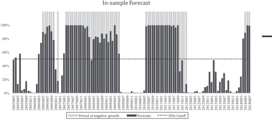
Now that a well-specified probit model has been selected, the next step is to evaluate its forecasting abilities. Preliminary tests with models containing more than three input variables have shown that models with high explanatory power are not necessarily suitable for forecasting purposes, especially when it comes to predicting market turning points. First, the selected model is tested for its gains over a constant probability model, also referred to as the naïve model, which makes predictions based only on a constant probability, i.e. it assumes rising prices for every observation period.Exhibit 7presents the prediction results in contrast to the constant probability model.

As can be seen on the right-hand-side of Exhibit 7, among the 112 observation periods a total of 55 periods experienced negative growth, which reflects a proportion of 49.1 per cent. Following this, the cut-off point is set to 0.5, which means that probabilities of 50 per cent and above are intended to indicate falling house prices. The model achieves total in-sample prediction correctness, i.e. the percentage of correct forecasts, of 89.3 per cent, which translates to correctly predicting 100 out of the 112 monthly observations within the observation period. It thereby achieves a significant gain over the naïve model of 38.4 per cent, which is only able to correctly predict 50.9 per cent of all periods. Furthermore, the mean-squared forecasting error is calculated, reflecting not only the correctness of the predictions (at the given cut off point) but providing insight into the overall accuracy of the predictions:

MSE⫽ 1 n兺

i⫽1 n

(A_i,t_⫹_m⫺ F_i,t_⫹_m)² (6) wheretis the point of time at which the prediction is made,mmarks the prediction horizon,A_i,t⫹mdenotes the actual realisations (as derived from the Case–Shiller House Price index) at timet⫹mandF_i,t_⫹_mthe forecasts. Because of the binary character of the probit model, A_i can only be either 1 or 0.F_i resembles a probability and can, therefore, only range between 0-100 per cent. ndenotes the number of observations within the forecast period. The in-sample MSE is reported at 0.07.Exhibit 8plots the in-sample forecast results for March 2005 to July 2014.

As is clearly evident, the few incorrect predictions were mostly around actual turning points, e.g. the beginning of negative growth phases in May 2006, March 2007 or the latest, one starting in May 2014.

Especially the beginning of the extreme drop in prices of 2006 following the bursting of the housing bubble would have been indicated by distinct signals with probabilities around 100 per cent. The only time the model suggests a switch from falling to rising prices a bit too soon, is the period around the beginning of 2012, when after a 20-month recession, prices started to pick up again in February 2012. Appendix 3shows the forecast results in comparison to the actual realisations of the Case–Shiller House Price Index.

5.2 Out-of-sample forecasts

Because one of the objectives of this study is to find a forecasting model that can be applied in practice, the model under review also needs to be tested for its out-of-sample forecasting performance. This is necessary, as it is the only way to realistically re-enact

IJHMA 9,1

118

(13)

real-time conditions in terms of data availability. The lowest lag order of our model is four months (Real Estate Listings subcategory), which automatically determines the maximum out-of-sample forecasting horizon. Thus, 1- to 4-month out-of-sample forecasts are conducted as “real-time” predictions. This means that, first, the model is estimated from the start of the observation sample up to June 2008. This can be considered as the estimation or training period. The model is then used to perform rolling projections one to four months ahead, starting from July 2008. This procedure is repeated over and over again, adding one more observation to the estimation (training) period with every new forecast, and thereby extending the training period with each extra step. From this point onwards, regressions are rolled through every following month, until the end of the estimation period in June 2014. Hence, the entire out-of-sample forecast period ranges from July 2008 to June 2014, which comprises a total of six years (72 observations).

By way of example, equation (7) shows the forecast equation for the first one-month-ahead out-of-sample prediction for July 2008.

Estimation sample January 2004-June 2008:

Pr_2008m07⫽ ⌽(␣ ⫹ ␤1G_APR_2007m07⫹␤2G_LIST_2008m03⫹ ␤3G_CONS_2007m10

⫹ ␧2008m07) (7)

The equation resembles the same lag structure as in equation (5). Note that the predicted probability is one month ahead of the estimation sample and thus “out-of-sample”. As mentioned above, the variable with the lowest lag order G_LIST (four lags) determines the maximum forecast horizon (Tsolacos, 2012). For an estimation sample of January 2004-June 2008, this would be October 2008. As the model is recursive, the presented equation variables in equation (7) advance one month with every further step.

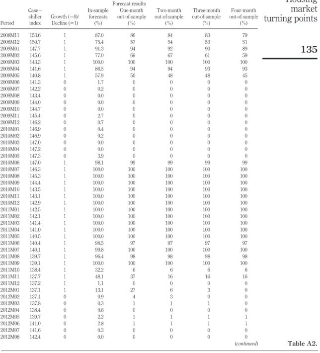
During the out-of-sample period of six years, three phases of negative growth took place, as can be seen inExhibit 9. The two- to four-month-ahead forecast results can be found inAppendices 2and3.

Overall, the prediction accuracy of the one-month-ahead out-of-sample forecasting model for this time period is 88.9 per cent and thus only slightly less than the in-sample prediction accuracy. As expected, the MSE of 0.082 is slightly larger than that in the in-sample forecast. Very similar to the in-sample forecasts, most of the incorrect predictions occur towards the beginning or end of a negative growth phase. In accordance with the in-sample results, the model, for example, already suggests a switch from decline to growth in October 2011, although prices did not start to rise until February 2012. Similarly, but not quite as early, it would have predicted a switch one month ahead early in May 2009 and April 2014. Although not very strong (71 and 53 per cent), the only exceptions where incorrect predictions do not occur around an actual turning point are two false signals in February and March 2013. Thus, one important finding should be mentioned; apart from the two false signals that have just been pointed out, the remaining incorrect predictions are always early, and never late. This is an important fact, when it comes to judging the model’s ability as an early indicator of upcoming switches from a phase of price growth to one of decline and vice versa. The results for the two- to four-month forecasts are in line with this finding (Appendices 2 and3).

119 Housing market turning points

(14)

As it has now been established that a probit model based on real-estate-specific Google search volume data is able to deliver satisfactory forecasting results and can be used to predict turning points in prices of the US housing market, another handy advantage of Google data should be mentioned. While the Case–Shiller House Price Index is released with an approximate two-month delay, Google search volume data are available after only two days. This means a time advantage of nearly two months in addition to the four-month prediction horizon of the suggested model. As outlined in Exhibit 10, with respect to forecasting the Case–Shiller House Price Index, the first two months can (due to the time delay) be considered a “nowcast”, and the following four months an actual “forecast”. Consequently, because the model is based on Google data only, the prediction horizon increases to six months.

6. Conclusion

The world has fairly recently experienced and suffered from the devastating economic aftermath of a bursting real estate bubble in the USA. This demonstrated the incredible impact the housing market can have on an economy and how important it is to monitor its development. If the pending major price correction of the US housing market had been indicated to a broader public in 2005, politically driven economic adjustments might have prevented, or at least alleviated, one of the worst economic crises since the early twentieth century.

This paper focuses on analysing turning points in the housing market, which, to date, is a fairly under-researched subject. Furthermore, it deploys a relatively new set of sentiment indicators, namely, Google search volume, which offers some advantages over other more common sentiment indicators, particularly in terms of availability, timing and its high degree of flexibility in extracting information. One of the main objectives is to find a forecasting model that is able to produce reliable real-time predictions of turning points in the US housing market.

For this purpose, binary probit models, which are geared specifically towards predicting directional changes, are used as a forecasting tool. WhileKrystalogianniet al.

(2004),Tsolacos (2012)andTsolacoset al.(2014)confirm the usefulness of probit models for turning-point predictions in the commercial real estate market, this paper is the first to apply this methodology to the housing market, and with promising results. After selecting a multivariate probit model, which is based on three individual real-estate-related Google search indices, a number of in- and out-of-sample tests provide evidence that online search data serve as a robust indicator for predicting directional changes in the housing market. The out-of-sample-forecast tests of one- to four-month forecasts demonstrate that the selected model correctly predicts 89 per cent of the time. Most importantly, however, apart from two false predictions (assuming a cut off point at 0.5) in 2012, the model indicates every upcoming turning point correctly, while the few signals that are slightly off on the timing are always early, but never late.

This clearly indicates that real-estate-specific internet search interest has the ability to serve as a robust indicator for future upcoming house price changes. Moreover, due to the immediate availability of Google data, in contrast to the two-month-delayed Case–

Shiller House price index, the effective prediction horizon increases to six months.

The results are relevant to a large number of stakeholders in the housing market, including developers, policymakers and, of course, prospective buyers and sellers. With respect to its applicability in practice, particularly investors with short investment

IJHMA 9,1

120

(15)

horizons (“house flipping”) and also lenders can potentially profit from the presented concept. Especially in light of the recent US housing bubble that mainly resulted from the combination of high loan-to-equity ratios and rapidly declining prices, lenders have learned for the future and will very likely adjust their pricing and lending standards more carefully and prudently, and in accordance with the market outlook.

Because the effective prediction horizon is six months, the findings of this research could also be relevant to investors who trade Case–Shiller House-Price-Index-based derivatives (futures and options) as offered by the CME group. Because the expiration dates are February, May, August and November, six months could potentially be long enough for an investor to estimate whether or not those products are fairly priced.

Future research should exploit the unique features of Google search volume data and make use of the flexibility of search indices, which can be configured very individually by simply combining different search queries. This, in combination with an intelligent use of filters (e.g. regional and topic filters), creates the opportunity to take the present research to an MSA/city level and thus become more appealing to private and institutional investors or local policymakers, given the heterogeneity of local real estate markets across the USA. Particularly, the respective relationships between very liquid and dynamic markets (e.g. San Francisco, NYC), in comparison to more stable markets which experience lower levels of market activity, and region-specific Google search volume constitute an interesting field for further research.

Notes

1. According to comScore, the market share of Google sites is 67.3 per cent with approximately 12.1 billion explicit searches:www.comscore.com/Insights/Market-Rankings/comScore- Releases-August-2014-US-Search-Engine-Rankings

2. www.conference-board.org/data/consumerconfidence.cfm 3. www.sca.isr.umich.edu/

4. The changes in the search indices are minor and practically negligible, especially when converted to monthly data. The joint correlation of every search index used in this present study across the index downloads from different days lies above 0.99.

5. In the case of an unchanged index (i.e. a growth rate of zero per cent), the binary time series is ascribed a value of zero.

6. In this current research,kis set to a maximum of three in the multivariate probit models.

7. The analysis was limited to three explanatory variables, as goodness-of-fit tests showed that models including more than three variables are largely over-specified. Furthermore, parsimonious models, which are also preferred by the literature (Tsolacos et al., 2014), perform better in out-of-sample forecasts, which was also confirmed in preliminary tests.

References

Amihud, Y. (2002), “Illiquidity and stock returns: cross-section and time-series effects”, The Journal of Financial Markets, Vol. 5 No. 1, pp. 31-56.

Anderson, H.A., Athanasopoulos, G. and Vahid, F. (2007), “Nonlinear autoregressive leading indicator models of output in G-7 countries”,Journal of Applied Econometrics, Vol. 22 No. 1, pp. 63-87.

121 Housing market turning points

(16)

Andrews, D.W.K. (1988), “Chi-square diagnostic tests for econometric models: theory”, Econometrica, Vol. 56 No. 6, pp. 1419-1453.

Baker, S.R. and Fradkin, A. (2011), “What drives job search? Evidence from Google search data”, Working Paper, Stanford Institute for Economic Policy Research, Stanford, available at:

SSRNeLibrary.

Bandholz, H. and Funke, M. (2003), “In search of leading indicators of economic activity in Germany”,Journal of Forecasting, Vol. 22 No. 4, pp. 277-297.

Banerjee, A. and Marcellino, M. (2006), “Are there any reliable leading indicators for US inflation and GDP growth?”,International Journal of Forecasting, Vol. 22 No. 1, pp. 137-151.

Barber, B., Odean, T. and Zhu, N. (2009), “Do retail trades move markets?”,Review of Financial Studies, Vol. 22 No. 1, pp. 151-186.

Beracha, E. and Wintoki, B.M. (2013), “Forecasting residential real estate price changes from online search activity”,Journal of Real Estate Research, Vol. 35 No. 3, pp. 283-312.

Brown, S.J., Goetzmann, W.N., Hiraki, T., Shiraishi, N. and Watanabe, M. (2003), “Investor sentiment in Japanese and US daily mutual fund flows”, NBER Working Paper No. 9470, Cambridge.

Carrière-Swallow, Y. and Labbé, F. (2013), “Nowcasting with Google Trends in an Emerging Market”,Journal of Forecasting, Vol. 32 No. 4, pp. 289-298.

Case, K.E. and Shiller, R.J. (2003), “Is there a bubble in the housing market? An analysis”, Brookings Papers on Economic Activity, Vol. 34 No. 2, pp. 299-362.

Chauvet, M. and Potter, S. (2005), “Forecasting recessions using the yield curve”, Journal of Forecasting, Vol. 24 No. 7, pp. 77-103.

Chen, S. (2009), “Predicting the bear stock market: macroeconomic variables as leading indicators”,Journal of Banking & Finance, Vol. 33 No. 2, pp. 211-223.

Choi, H. and Varian, H. (2012), “Predicting the present with Google trends”,The Economic Record, Vol. 88 No. 1, pp. 2-9.

Chopra, N., Lee, C.M., Shleifer, A. and Thaler, R. (1993), “Yes, discounts on closed-end funds are a sentiment index”,The Journal of Finance, Vol. 48 No. 2, pp. 801-808.

Clayton, J. (1996), “Rational expectations, market fundamentals and housing price volatility”,Real Estate Economics, Vol. 24 No. 4, pp. 441-470.

Clayton, J. (1997), “Are housing price cycles driven by irrational expectations?”,Journal of Real Estate Finance and Economics, Vol. 14 No. 3, pp. 341-363.

Clayton, J. (1998), “Further evidence on real estate market efficiency”, Journal of Real Estate Research, Vol. 15 No. 1, pp. 41-57.

Clayton, J., Ling, D.C. and Naranjo, A. (2009), “Commercial real estate valuation: fundamentals versus investor sentiment”,The Journal of Real Estate Finance and Economics, Vol. 38 No. 1, pp. 5-37.

Croce, R.M. and Haurin, D.R. (2009), “Predicting turning points in the housing market”,Journal of Housing Economics, Vol. 18 No. 4, pp. 281-293.

Da, Z., Engelberg, J. and Gao, P. (2011), “In search of attention”,The Journal of Finance, Vol. 66 No. 5, pp. 1461-1499.

Da, Z., Engelberg, J. and Gao, P. (2013), “The sum of all fears: investor sentiment and asset prices”, Review of Financial Studies, Vol. 28 No. 1.

Dietzel, M.A., Braun, N. and Schaefers, W. (2014), “Sentiment-based commercial real estate forecasting with Google search volume data”,Journal of Property Investment & Finance, Vol. 32 No. 6, pp. 540-569.

IJHMA 9,1

122

(17)

Drake, M.S., Roulstone, D.T. and Thornock, J.R. (2012), “Investor information demand: evidence from Google searches around earning announcements”,Journal of Accounting Research, Vol. 50 No. 4, pp. 1001-1040.

Estrella, A. and Mishkin, F.S. (1998), “Predicting US recessions: financial variables as leading indicators”,Review of Economics and Statistics, Vol. 80 No. 1, pp. 45-61.

Filardo, A.J. (1999), “How reliable are recession prediction models?”,Federal Reserve Bank of Kansas City Economic Review, Vol. 84 No. 2.

Frazzini, A. and Lamont, O.A. (2008), “Dumb money: mutual fund flows and the cross-section of stock returns”,Journal of Financial Economics, Vol. 88 No. 2, pp. 299-322.

Ginsberg, J., Mohebbi, M.H., Patel, R.S., Brammer, L., Smolinski, M.S., Brilliant, L. and Zimmermann, K.F. (2009), “Detecting influenza epidemics using search engine query data”, Nature, Vol. 457 No. 1.

Hodrick, R.J. and Prescott, E.C. (1997), “Postwar US business cycles: an empirical investigation”, Journal of Money, Credit and Banking, Vol. 29 No. 1, pp. 1-16.

Hohenstatt, R. and Käsbauer, M. (2014), “GECO’s weather forecast for the UK housing market: to what extent can we rely on Google econometrics?”,Journal of Real Estate Research, Vol. 36 No. 2, pp. 253-281.

Hohenstatt, R., Käsbauer, M. and Schäfers, W. (2011), “’GECO’ and its potential for real estate research: evidence from the US housing market”,Journal of Real Estate Research, Vol. 33 No. 4, pp. 471-506.

Jin, C., Soydemir, G. and Tidwell, A. (2014), “The US housing market and the pricing of risk:

fundamental analysis and market sentiment”,Journal of Real Estate Research, Vol. 36 No. 2, pp. 187-216.

Jones, C.M. and Lamont, O.A. (2002), “Short sale constraints and stock returns”, Journal of Financial Economics, Vol. 66 Nos 2/3, pp. 207-239.

Jurgilas, M. and Lansing, K.J. (2013), “Housing bubbles and expected returns to homeownership:

lessons and policy implications”, Working Paper, available at SSRN: eLibrary.

Kaplanski, G. and Levy, H. (2014), “Seasonality in perceived risk: a sentiment effect”, Working Paper, available at SSRN: eLibrary.

Kouwenberg, R. and Zwinkels, R. (2014), “Forecasting the US housing market”,International Journal of Forecasting, Vol. 30 No. 3, pp. 415-425.

Krystalogianni, A., Matysiak, G. and Tsolacos, S. (2004), “Forecasting UK commercial real estate cycle phases with leading indicators: a probit approach”,Applied Economics, Vol. 36 No. 20, pp. 2347-2356.

Lee, C.M.C., Shleifer, A. and Thaler, R.H. (1991), “Investor sentiment and the closed-end fund puzzle”,The Journal of Finance, Vol. 46 No. 1, pp. 75-109.

Lemmens, A., Croux, C. and Dekimpe, M.G. (2005), “On the predictive content of production surveys: a pan-European study”, International Journal of Forecasting, Vol. 21 No. 2, pp. 363-375.

Ling, D.C., Ooi, J.T.L. and Le, T.T.T. (2014), “Explaining house price dynamics: isolating the role of non-fundamentals”,Journal of Money, Credit, and Banking, Vol. 47 No. 1.

Marcato, G. and Nanda, A. (2014), “Information content and forecasting ability of sentiment indicators: case of real estate market”,Journal of Real Estate Research, Vol. 1 No. 1.

Matysiak, G. and Tsolacos, S. (2003), “Identifying short-term leading indicators for real estate rental performance”,Journal of Property Investment and Finance, Vol. 21 No. 3, pp. 212-232.

123 Housing market turning points

(18)

Nanda, A. (2007), Examining the NAHB/Wells Fargo Housing Market Index (HMI), Housing Economics, National Association of Home Builders, WA, DC, March 2007.

Neal, R. and Wheatley, S.M. (1998), “Do measures of investor sentiment predict returns?”,Journal of Financial and Quantitative Analysis, Vol. 33 No. 4, pp. 523-547.

Nyberg, H. (2010a), “Dynamic probit models and financial variables in recession forecasting”, Journal of Forecasting, Vol. 29 Nos 1/2, pp. 215-230.

Nyberg, H. (2010b), “Forecasting the direction of the US stock market with dynamic binary probit models”,International Journal of Forecasting, Vol. 27 No. 2, pp. 561-578.

Preis, T., Moat, H.S. and Stanley, E. (2013), “Quantifying trading behavior in financial markets using Google trends”,Nature – Scientific Reports, Vol. 3 No. 1684, pp. 1-6.

Randall, R.J., Suk, D.Y. and Tully, S.W. (2003), “Mental fund cash flows and stock market performance”,Journal of Investing, Vol. 12 No. 1, pp. 78-81.

Rochdi, K. and Dietzel, M.A. (2015), “Outperforming the benchmark: online information demand and REIT market performance”,Journal of Property Investment and Finance, Vol. 33 No. 2, pp. 169-195.

Shiller, R.J. (2007), “Understanding recent trends in house prices and home ownership”, paper presented at the Federal Reserve Bank of Kansas City’s Jackson Hole Symposium, Kansas, 31 August – 1 September.

Shiller, R.J. (2008), “Historic turning points in real estate”,Eastern Economic Journal, Vol. 34 No. 1, pp. 1-13.

Taylor, K. and McNabb, R. (2007), “Business cycles and the role of confidence: evidence for Europe”,Oxford Bulletin of Economics and Statistics, Vol. 69 No. 2, pp. 185-208.

Tsolacos, S. (2012), “The role of sentiment indicators for real estate market forecasting”,Journal of European Real Estate Research, Vol. 5 No. 2, pp. 109-120.

Tsolacos, S., Brooks, C. and Nneji, O. (2014), “On the predictive content of leading indicators: the case of US real estate markets”,Journal of Real Estate Research, Vol. 36 No. 4, pp. 541-573.

Weber, W. and Devaney, M. (1996), “Can consumer sentiment surveys forecast housing starts?”, Appraisal Journal, Vol. 4 No. 1, pp. 343-350.

Whaley, R.E. (2009), “Understanding VIX”, Journal of Portfolio Management, Vol. 35 No. 3, pp. 98-105.

Wheaton, C.W. and Nechayev, G. (2008), “The 1998 –2005 housing ‘Bubble’ and the current

‘correction’: what’s different this time?”,Journal of Real Estate Research, Vol. 30 No. 1, pp. 1-26.

Wu, L. and Brynjolfsson, E. (2014), “The future of prediction: how Google searches foreshadow housing prices and sales”,Economics of Digitization, University of Chicago Press, Chicago.

IJHMA 9,1

124

(19)

Exhibit 1

–40 –30 –20 –10 0 10 20 30 40

2005M03 2005M06 2005M09 2005M12 2006M03 2006M06 2006M09 2006M12 2007M03 2007M06 2007M09 2007M12 2008M03 2008M06 2008M09 2008M12 2009M03 2009M06 2009M09 2009M12 2010M03 2010M06 2010M09 2010M12 2011M03 2011M06 2011M09 2011M12 2012M03 2012M06 2012M09 2012M12 2013M03 2013M06 2013M09 2013M12 2014M03

Case-Shiller House Price Index Google Real Estate Category

Note: This graph depicts the Case-Shiller House Price Index and the Google search volume index for the real estate subcategory in terms of annual changes

Figure E1.

Case–Shiller House Price Index vs Google real estate category

International Journal of Housing Markets and Analysis