Risk Management in International Real Estate and Capital Markets

I

Risk Management in International Real Estate and Capital Markets

Dissertation zur Erlangung des Grades eines Doktors der Wirtschaftswissenschaft

eingereicht an der Fakultät für Wirtschaftswissenschaften der Universität Regensburg

vorgelegt von:

Cay Philip Oertel

Berichterstatter:

Prof. Dr. Sven Bienert, Universität Regensburg Prof. Dr. Steffen Sebastian, Universität Regensburg

Tag der Disputation:

22. Juli 2020

Contents

List of Tables ...III List of Figures ... IV

1 Introduction ...1

1.1 Risk in real estate, the impact of securitization and derived research ...2

1.2 Bibliography ...7

2 The relationship between domestic and global Economic Political Uncertainty and European Direct Commercial Real Estate Returns ...9

2.1 Introduction ... 10

2.2 Theoretical background, related literature and hypotheses derivation ... 11

2.3 Research design and measurement of uncertainty ... 15

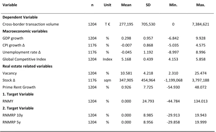
2.4 Data and descriptive statistics ... 17

2.5 Methodology ... 20

2.6 Empirical results ... 21

2.7 Conclusion and further remarks ... 24

2.8 Bibliography ... 28

2.9 Appendix ... 32

3 Do Cross-Border Investors Benchmark Commercial Real Estate Markets? Evidence from Relative Yields and Risk Premia for a European Investment Horizon ... 33

3.1 Introduction ... 34

3.2 Related literature and hypotheses derivation ... 35

3.3 Data, sample description and methodology ... 38

3.4 Empirical results ... 46

3.5 Conclusion and further aspects ... 53

3.6 Bibliography ... 55

3.7 Appendix ... 58

4 Volatility Targeting for US Equity REITs – A strategy for Minimizing Extreme Downside Risk? ... 59

II

4.4 Methodology ... 66

4.5 Empirical results ... 68

4.6 Conclusion, practical implications and further research ... 75

4.7 Bibliography ... 77

4.8 Appendix ... 80

5 AR-GARCH-EVT-Copula for Securitized Real Estate: An approach to improving risk forecasts? .... 83

5.1 Introduction ... 84

5.2 Literature review and hypothesis derivation ... 86

5.3 Methodology ... 86

5.4 Data and descriptive statistics ... 96

5.5 Empirical results ... 99

5.6 Conclusion ... 111

5.7 Bibliography ... 113

5.8 Appendix ... 118

6 Conclusion ... 119

6.1 Conclusion ... 120

6.2 Bibliography ... 124

Table 1: Data description and variable selection for total return models ... 17

Table 2: Descriptive statistics for variables of the total return models ... 18

Table 3: Correlation matrix of the total return data set ... 19

Table 4: Pooled OLS estimation results (total return) ... 22

Table 5: Explanatory power of total return models without DEPUI / GEPUI ... 24

Table 6: Levin-Lu-Chu stationarity test for total return model variables ... 32

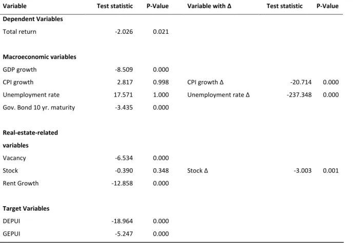
Table 7: Control variable description for cross-border volume models ... 42

Table 8: Descriptive statistics for variables of the cross-border transaction volume models ... 43

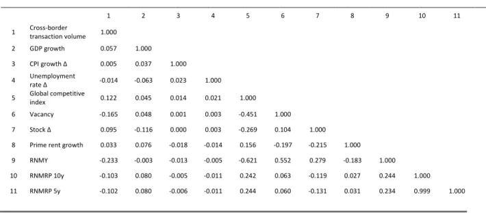
Table 9: Correlation matrix for cross-border transaction volume model variables ... 44

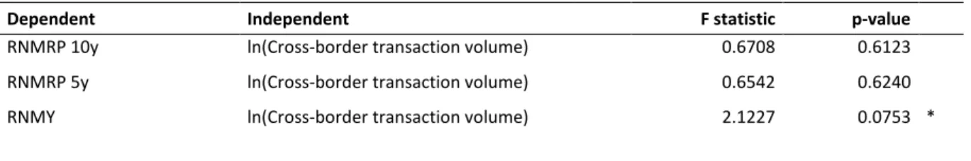
Table 10: Granger causality test (RNMRP & RNMY – cross-border transaction volume) ... 46

Table 11: Pooled OLS estimation results (cross-border transaction volume) ... 47

Table 12: GAMM estimation results for penalized spline functions of non-parametric covariates ... 50

Table 13: Levin-Lin-Chu stationarity test for cross-border transaction volume model variables ... 58

Table 14: Descriptive statistics of daily US equity REIT returns (01/01/1999 – 01/01/2019)... 64

Table 15: Maximum STARR (Buy and Hold & VT (hist. Vol, VIX & GARCH)) ... 74

Table 16: Correlation matrix (Office REITs) ... 80

Table 17: Correlation matrix (Residential REITs) ... 80

Table 18: Correlation matrix (Industrial REITs) ... 80

Table 19: Correlation matrix (Retail REITs) ... 81

Table 20: Correlation matrix (Diversified REITs) ... 82

Table 21: Correlation matrix (Health Care REITs) ... 82

Table 22: Correlation matrix (Lodging & Resorts REITs) ... 82

Table 23: Descriptive statistics ... 98

Table 24: Empirical results for VaR forecasts ... 101

Table 25: Empirical results for CVaR forecasts ... 104

Table 26: Results of the autoregressive modelling ... 106

Table 27: Empirical results for the copulae estimation ... 109

Table 28: List of applied copulae ... 118

IV

Figure 1: Adjusted GEPUI scores (Q1/2008 – Q3/2018) ... 16

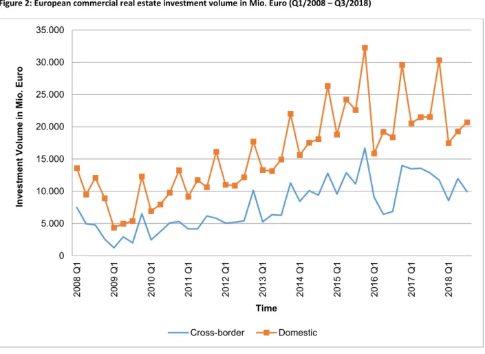
Figure 2: European commercial real estate investment volume in Mio. Euro (Q1/2008 – Q3/2018) .. 39

Figure 3: Penalized spline functions of RNMPR 10y and RNMRP 5y – models G.2 & G.3 ... 51

Figure 4: Efficiency frontiers within mean-CVaR0.95-framework (All REITs) ... 69

Figure 5: Efficiency frontiers within mean-CVaR0.95-framework (Office REITs) ... 70

Figure 6: Efficiency frontiers within mean-CVaR0.95-framework (Retail REITs) ... 70

Figure 7: Efficiency frontiers within mean-CVaR0.95-framework (Industrial REITs) ... 71

Figure 8: Efficiency frontiers within mean-CVaR0.95-framework (Residential REITs) ... 71

Figure 9: Efficiency frontiers within mean-CVaR0.95-framework (Diversified REITs) ... 72

Figure 10: Efficiency frontiers within mean-CVaR0.95-framework (Lodging and Resort REITs) ... 72

Figure 11: Efficiency frontiers within mean-CVaR0.95-framework (Health Care REITs) ... 73

Figure 12: VaR0.95 estimates for Real Estate–Stocks portfolio (US) ... 85

Figure 13: Cumulated return series for real estate, stocks and bonds (US) ... 97

Figure 14: VaR0.95-fr estimates for Real Estate – Stocks & Real Estate - Bonds portfolio (US) ... 100

1 Introduction

2

1.1 Risk in real estate, the impact of securitization and derived research

The presence of risk is an essential part of finance since risk-taking is the natural economic necessity to generate excess returns (dating back to Knight, 1921). Although a single and unanimously accepted definition of the term is missing across different sciences, the meaning of risk in finance entails two decisive elements: The potential of a negative divergence from expected values and a corresponding monetary loss due to the negative divergence (McNeil et al., 2015).

Based on these two components, the term risk in academia is strongly connected to uncertainty and randomness. Investors face situations in which the future financial performance of assets, like real estate, is uncertain. Thus, any decision entails ex ante uncertainty about its outcome in the future. In terms of statistical language and real estate, the interpretation is that these risks or concrete risk factors, such as rental growth, maintenance expenses, construction costs, financing costs, etc., are modelled as random variables (French & Gabrielli, 2004).

Financial risk management has focused on the application of probability theory to model these random variables in a decision under uncertainty. According models were introduced by Kolmogorov (1933) to oppose purely deterministic models. This pioneering work still provides the common terminology for risk-related scientific discussion. The application of probability in the real estate literature and in the context of risk represents the class of so-called stochastic models. In contrast to deterministic models, their stochastic peers allow the explicit modelling of risk using the corresponding distribution functions of the risk factors in the future to account for their randomness (Pfnür & Armonat, 2013).

The financial risk management of investment positions is implemented in practice by institutional investors using a comprehensive and recursive risk management system, which is supposed to ensure the identification, quantification, steering, and surveillance of risks. This procedure applies to investors of classic capital market products, such as stocks or bonds and alternatives, like real estate mostly alike, because legal requirements generally do not differ between the assets of the investment company. In this context, a clear development of legal tightening can be observed in the aftermath of the global financial crisis in 2008.

Additionally, risk management has moved into the center of attention from an economic point of view because of concerns about potential over-valuations of property assets have risen due to the extensive global monetary expansion (Hayunga & Lung, 2011;

Abildgren et al., 2018; Fabozzi & Xiao, 2019) and the economic turmoil due to the COVID-19 pandemic.

1 In Germany, for example, the introduction of the “Kapitalanlagegesetzbuch” in 2013, and subsequently the

“Mindestanforderungen an das Risikomanagement von Kapitalverwaltungsgesellschaften” in 2017. Both regulatory adjustments are based on European law, namely the Alternative Investment Fund Manager Directive (AIFMD), illustrating an international scale of regulation.

However, the concrete methodological implementation of a stochastic approach is subject to the asset class specifics of the managed positions. These asset class specifics are highly relevant for the present thesis because the articles address the abovementioned types of products: Firstly, alternative investments like direct real estate and secondly, classic investment products like stocks including securitized real estate and bonds. The decisive mechanism that separates the articles and the methodology is the securitization function of indirect investment vehicles in capital markets. On the one hand, direct real estate as an asset class can be characterized as heterogeneous, illiquid, having high transaction costs and durations, and entailing low fungibility and transparency (or information respectively), among others. Indirect or securitized real estate, on the other hand, transforms these specifics of the underlying assets. Accordingly, the risk management methodology changes as well, because capital markets provide homogeneity, liquidity, fungibility, information, relatively low transaction costs and durations. Lastly, debt positions focus methodologically on aspects arising from the individual credit agreement and the borrower, urging to model metrics like probability of default (PD), loss given default (LGD) or exposure at default (EAD), etc. (for a summary see Booth et al., 2002).

The modelling within the real estate industry focused historically on qualitative approaches to manage the risk of their positions. However, due to the legal requirements as well as higher data availability and probability functions of risk factors (Amédée-Manesme & Barthélémy, 2018), more quantitative approaches including stochastic modelling in the sense of Kolmogorov (1933) have been established.

Accordingly, for direct real estate, the most feasible stochastic approach to quantify the residual risk of the assets is the Monte Carlo Simulation (MCS; Hoesli et al., 2006; Baroni et al., 2007). For the simulation of the cash flows of the properties, however, the macroeconomic environment and the relevant risk factors of the assets need to be identified correctly because real estate assets are highly dependent on the macroeconomic circumstances. Central for this modelling is the question, what risk factors can affect the cash flows of the property? Therefore, it is crucial to identify the functional chain in risk factors models (e.g., as described by Ho et al., 2015) before quantifying the impact on the individual asset level. The thesis derived the following selected aspects of risk management in international real estate and capital markets based on these considerations of risk identification, quantification, steering, and surveillance in direct as well as securitized real estate markets.

The first article of the thesis presents a typical fundamental risk factor model described above. It aims

at assessing the potential impact of domestic and global economic political uncertainty on commercial

real estate markets. Recently, politics-related uncertainties like Brexit have gained large interest

(French, 2019). However, the existing body of literature has mainly focused on residential markets in

this context (e.g., Monfared & Pavlov, 2019). Thus, the paper “The relationship between domestic and

4

Europe. Additionally, the independent covariates are divided into domestic and global economic political uncertainty to find thinkable cross-border effects of uncertainty after controlling for the domestic peer to detect a potential “safe haven effect,” namely a positive influence of foreign uncertainty on domestic properties.

The second article on direct property markets “Do Cross-Border Investors Benchmark Commercial Real Estate Markets? Evidence from Relative Yields and Risk Premia for a European Investment Horizon”

addresses the determinants of cross-border investment flows in real estate markets. So far, literature has widely focused on economic or institutional pull factors, which attract capital (e.g., Lieser & Groh, 2014). The article extends the existing literature by constructing a synthetic index for European investment locations to test for the relative attractiveness of a market as a determinant of inflowing capital. Methodologically, linear as well as non-linear regression models are used for European panel data. Nonetheless, one may ask about the connection between foreign capital flows and risk management. Market liquidity of direct real estate markets can be an important risk factor, which may cause deviations from expected values of, e.g., transaction durations, time on the market, etc. Thus, the article contributes to the understanding of the underlying functional chain of market liquidity, which is a commonly known risk factor.

Next, the thesis turns towards the risk management of securitized real estate positions in capital markets. As outlined above, the transformation functions of indirect vehicles allow investors to steer the risk of their indirect positions differently from their direct peers. Here, the paper “Volatility Targeting for US Equity REITs – A Strategy for Minimizing Extreme Downside Risk?” presents the so- called Volatility Targeting rebalancing algorithm for REIT securities as an active management tool for risk steering. Since daily returns of REITs are showing even stronger volatility clustering and leverage effect than classic equities (Cotter & Stevenson, 2007; Jirasakuldech et al., 2009), the asset class appears to be very promising for research on volatility-based risk strategies. To the author’s knowledge, no article has carried out an empirical study on the specified technique of REIT securities to analyze the characteristics of REIT volatility explicitly from an applied risk management point of view. To provide insight, at first a back testing approach simulates returns from the volatility targeting algorithm. The strategy bases on various volatility estimators, such as historical volatility, the CBOE Volatility Index based on broader stock market option prices, and on one-day-ahead forecasts of a generalized autoregressive conditional heteroscedasticity (GARCH) model. The realized returns of the strategies are then analyzed in a portfolio optimization framework to identify the strategies’ economic efficiency compared to a classic buy and hold investment scenario.

The last paper extends the investment horizon to classic stocks and bond positions. The paper “AR-

GARCH-EVT-Copula for Securitized Real Estate: An approach to improving risk forecasts” is the first

study to apply the so-called AR-GARCH-EVT-Copula model to bivariate portfolios, which contain securitized real estate in addition to the abovementioned capital market products. Different from the previous article, this paper does not aim at economic efficiency and its frontiers but forecasting risk metrics. The primary motivation for the paper is the stylized facts about financial market data. The data have repeatedly shown leptokurtosis, skew and fat tails (largely discussed by McNeil & Frey, 2000), which provokes the application of a GARCH-standardization to model the dependency of securitized real estate and other asset classes. In addition, dynamic and asymmetric dependency appears to be necessary since real estate is an asset class, which co-moves to stocks and bonds in timely variant, skewed, and over-proportional fashion. The approach aims at solving for the named issues and compares the method to classic historical simulation or variance-covariance method to obtain risk metric forecasts. Based on the entire aforementioned derived research, the following questions are central for the empirical studies of the thesis:

1. The relationship between domestic and global Economic Political Uncertainty and European Direct Commercial Real Estate Returns

I. Does domestic economic political uncertainty affect total returns of direct office property investments?

II. Is foreign economic political uncertainty a driver of domestic direct commercial property returns?

2. Do Cross-Border Investors Benchmark Commercial Real Estate Markets? Evidence from Relative Yields and Risk Premia for an European Investment Horizon

I. Is there a relationship between the relative yield or risk premia attractiveness of an investment location and inflowing cross-border transaction volumes?

II. Is there empirical evidence for a non-linear relationship between the relative attractiveness proxy and inflowing cross-border transaction volumes?

III.

3. Volatility Targeting for US Equity REITs – A Strategy for Minimizing Extreme Downside Risk?

I. Is the application of Volatility Targeting for US Equity REITs economically efficient compared to a benchmark buy and hold strategy in a mean-tail-risk-optimization framework?

II. What volatility measurement provides the highest economic efficiency in the mean-tail-risk-

6

4. AR-GARCH-EVT-Copula for Securitized Real Estate: An approach to improving risk forecasts?

I. Does the AR-GARCH-EVT-Copula approach provide more accurate risk metric forecasts compared to the variance-covariance or historical simulation method?

The thesis is structured as follows to provide insight. The next chapters reproduce the empirical studies

that are related to the abovementioned research questions. Every article is introduced by a page that

states the full list of authors in the order of the publication, the status of the article, and a short

abstract. The abstract matches the submitted or published article abstract in case the respective

medium reports an abstract. In case this does not apply, an unpublished abstract has been added. The

last chapter contains the conclusion stating a summary of the articles, the definite answer of the

derived hypothesis, the joint conclusions of the thesis, the research limitations, and potential future

research in real estate risk management.

1.2 Bibliography

Abildgren, K., Hansen, N. L., & Kuchler, A. (2018). Overoptimism and house price bubbles. Journal of Macroeconomics, 56(1), pp. 1–14.

Amédée-Manesme, C.H. & Barthélémy, F. (2018). Ex-ante real estate Value at Risk calculation method.

Annals of Operations Research, 262(2), pp. 257–285.

Baroni, M., Barthélémy, F., & Mokrane, M. (2006). Monte Carlo Simulations versus DCF in Real Estate Portfolio Valuation. ESSEC Working Papers. Cergy-Pontoise.

Booth, P., & Matysiak, G., Ormerod, P. (2002). Risk Measurement and Management for Real Estate Porfolios. Investment Property Forum. London.

Cotter, J., & Stevenson, S. (2007). Uncovering Volatility Dynamics in Daily REIT Returns. The Journal of Real Estate Portfolio Management, 13(2), pp. 119–128.

Fabozzi, F. J., & Xiao, K. (2019). The Timeline Estimation of Bubbles: The Case of Real Estate. Real Estate Economics, 47(2), pp. 564–594.

French, N. (2019). Brexit and the Moon. Journal of Property Investment & Finance, 37(6), pp. 522–523.

French, N., & Gabrielli, L. (2004). The uncertainty of valuation. Journal of Property Investment &

Finance, 22(6), pp. 484–500.

Hayunga, D. K., & Lung, P. P. (2011). Explaining Asset Mispricing Using the Resale Option and Inflation Illusion. Real Estate Economics, 32(2), pp. 313–344.

Ho, D. K. & Addae-Dapaah, K. & Glascock, J. (2015). International Direct Real Estate Risk Premiums in a Multi-factor Estimation model. The Journal of Real Estate Finance and Economics, 51(1), pp.

52–85.

Hoesli, M., Jani, E., & Bender, A. (2006). Monte Carlo simulations for real estate valuation. Journal of Property Investment & Finance, 24(2), pp. 102–122.

Jirasakuldech, B., Campbell, R. D., & Emekter, R. (2009). Conditional Volatility of Equity Real Estate Investment Trust Returns: A Pre- and Post-1993 Comparison. The Journal of Real Estate Finance and Economics, 38(2), pp. 137–154.

Knight, F. H. (1921). Risk, uncertainty and profit. Mifflin. Boston & New York.

8

Kolmogorov, A. N. (1933). Sulla determinazione empirica di una legge di distribuzione. Giornale dell’Istituto Italiano degli Attuari, 4, pp. 83–91.

Lieser, K., & Groh, A. P. (2014). The Determinants of International Commercial Real Estate Investment.

The Journal of Real Estate Finance and Economics, 48(4), pp. 611–659.

McNeil, A. J., & Frey, R. (2000). Estimation of tail-related risk measures for heteroscedastic financial time series: an extreme value approach. Journal of Empirical Finance, 7(3), pp. 271–300.

McNeil, A. J., Frey, R., & Embrechts, P. (2015). Quantitative Risk Management. Priceton University Press. Princeton.

Monfared, S., & Pavlov, A. (2019). Political Risk Affects Real Estate Markets. The Journal of Real Estate Finance and Economics, 58(1), pp. 1–20.

Pfnür, A. & Armonat, S. (2013). Modelling uncertain operational cash flows of real estate investments using simulations of stochastic processes. Journal of Property Investment & Finance, 31(5), pp.

481–501.

2 The relationship between domestic and global Economic Political Uncertainty and European Direct Commercial Real Estate Returns

Cay Oertel, Sven Bienert, Werner Gleißner

Journal of European Real Estate Research (Revised)

Abstract

The aim of the study is to investigate the impact of domestic as well as global economic political

uncertainty on direct real estate returns at the European City-level. The empirical study uses OLS

estimation for a European direct real estate panel data set containing 20 cities across 9 European

countries, with quarterly observations from Q1/2008 – Q3/2018. After controlling for empirically

proven explanatory covariates of total returns, the model is extended by proxies for domestic and

global political uncertainty. The study finds c.p., on average a statistically significant lagged negative

influence of domestic economic political uncertainty on European direct commercial property total

returns. Global economic political uncertainty c.p. positively affects total returns, indicating a “safe

haven effect”.

10

2.1 Introduction

Economic political uncertainty (EPU) has recently moved into the center of attention. Brexit, the severe military tensions between the US and Iran, US-Chinese trade conflict, civil right activism in Hong Kong and persistent worrying signs from North Korea, all of which affect the international community are just a few prominent examples of a seemingly endless list of current political uncertainties with a potential economic impact. In this uncertain global environment, European real estate markets have been considered a “safe haven” for investors. Nonetheless, due to increased political uncertainties for example in the UK, the issue has reached European market participants as well (French, 2019). The question inevitably arises for market participants, as to whether and how this current domestic EPU (DEPU) is affecting real estate returns. The literature has repeatedly shown the impact of DEPU on direct residential property returns (e.g. Monfared & Pavlov, 2019). Does this also apply explicitly to commercial real estate returns and EPU in Europe?

Additionally, for various reasons not only domestic but also non-domestic or global economic political uncertainties (GEPU) may also reveal contagious spillover effects on European property returns. Most importantly, due to its central geographic location, Europe can be assumed to be exposed to GEPU.

Secondly, European economies are well-developed and thus globally integrated, for example through intense trade-related dependencies. Accordingly, these locations are expected to be more dependent on the global political environment, due to strong international economic connections (e.g. as recently discussed regarding European markets and the US by Oertel et al., 2019).

There is a literature on the impact of non-fundamental drivers such as EPU on real-estate-related parameters. However, these articles generally include market sentiment in terms of the economic environment, in order to quantify the impact on property market agents (e.g. Clayton et al., 2009;

Marcato & Nanda, 2016). To the best of the authors’ knowledge, there is no empirical study that isolates the impact of uncertainties from the economic political environment on direct commercial property returns. Accordingly, the central research question can be formulated as follows: Is there a statistically significant relationship between EPU and direct commercial real estate returns?

The article contributes to the existing body of literature in several ways. It is the first article to show

the relationship between European and especially city-level direct commercial property returns and

EPU at both the domestic and global levels. By contrast, previous articles have focused on national-

level index housing data in the US (e.g. Antonakakis et al., 2015). Secondly, not only country-specific

DEPU is assessed, but also GEPU as a potential factor that influences direct real estate returns. Thus,

the relationship is expanded by analyzing not only the relationship at the individual level, but also with

regard to the entire global environment.

The study is structured as follows. The next section outlines the theoretical related literature and derives the hypotheses for the empirical work. Based on the literature, the research design including the measurement for both types of EPU is described. The underlying data and the control variables for isolating the impact of the target variables are then explained. The ensuing sections contain the methodology and the empirical results. The final section concludes, describes practical implications and designs potential further research possibilities.

2.2 Theoretical background, related literature and hypotheses derivation

The present study considers total returns as the dependent variable of interest. The underlying theory for connecting EPU and returns stems mainly from a behavioral approach, which assumes investors to be affected by assumptions about future cash flows and investment risks (Baker & Wurgler, 2007). In order to derive the hypotheses and the methodological approach for a new empirical study, the literature on the following two issues needs to be considered: Theoretical transmission channels of DEPU and GEPU on total real estate returns, as well as existing empirical studies on other determinants of the specified returns. The latter part of the literature review is required to justify of the control variable set.

According to basic real estate theory, property returns are generated from changes in capital values and income (as formally expressed by the IPD):

𝑇𝑅_𝑡 =𝐶𝑉_𝑡− 𝐶𝑉_𝑡−1− 𝐶_{𝑒𝑥𝑝,𝑡}+ 𝐶_{𝑟𝑒𝑐,𝑡}+ 𝑁𝐼_𝑡 𝐶𝑉_𝑡−1+ 𝐶_{𝑒𝑥𝑝,𝑡}

(1)

where the total return, 𝑇𝑅

values can be broken down into more granular components, as formulated, for example, in Gunnelin et al. (2004):

𝐶𝑉_𝑡= ∑ 𝑅𝑡

(1 + 𝑖)^𝑡

𝑇

𝑡=1

+ 𝑅𝑇

(1 + 𝑖)^𝑇(𝑐 − 𝑔)

(2)

where

denotes the net rental income, discounted by the rate 𝑖. In the terminal period,

is

capitalized by an exit capitalization rate (𝑐) less an expected growth rate of cash-flows (𝑔). The exit

capitalization rate can further be decomposed by the Gordon model into risk-free interest 𝑟𝑓, and a

risk premium for placing capital in a property investment, 𝑟𝑝:

12

𝑐 = 𝑟𝑓 + 𝑟𝑝

(3)

Given these equations, the theoretical mechanisms for non-fundamental determinants such as EPU to affect the total returns, can be described. Firstly, the 𝐶𝑉

can be affected by the assumptions made by market participants about the abovementioned risky components of the future rental income components across the holding period,

income generation of commercial properties is time-lagged dependent on economic performance.

Economic performance again is partially a function of EPU (Smales, 2017). Secondly, increased uncertainty can also increase discount rates 𝑖, leading to a higher “penalization” of future cash-flows, and vice versa.

Lastly, the EPU can transmit through the exit capitalization (𝑐) of the property by means of a higher risk premium

assumptions and perceptions of market participants, as noted by Netzell (2009). Hence, it can be assumed from a theoretical point of view, that a statistically significant effect of EPU on the total returns is driven substantially by the appreciation return side. This assumption can be connected with the study of Chaney & Hoesli (2012), who identify the cap rates of commercial real estate as statistically significantly impacted by sentiment, thus potentially also by EPU. Since cap rates are highly relevant for the appreciation expressed in equations (2) and (3) above, this may provide an explanation. Due to the long-lasting nature of real estate rental agreements, however, this general finding should be evaluated as economically trivial.

For the income side on the other hand, the decisive determinants are net income receivables as a percentage of capital employed. These receivables from property investments are dependent on vacancy rates and expected rental growth (Gunnelin et al., 2004). Such receivables are theoretically potentially negatively affected by EPU through assumptions made by market agents, if potential tenants reduce their space demand or by negative rent growth, reducing 𝑁𝐼

. However, due to the above mentioned potential long-term rental agreements, especially short-term shocks in EPU are theoretically substantially eased for the income side of office property investments.

The empirical literature on non-fundamental determinants of property returns dates back to the work of Case & Shiller (1989), who introduce the impact of sentiment and the respective indices on residential property markets. Ensuing articles on residential and commercial real estate returns have broadly confirmed a statistically significant relationship between economic market sentiment and real estate market parameters and especially direct returns (e.g. Clayton et al., 2009; Tsolacos et al., 2014;

Ling et al., 2015; Marcato & Nanda, 2016).

Based on this broader term of market sentiment, the politics-related component of DEPU has been analyzed in only a few articles in the real estate literature. Monfared & Pavlov (2019) recently showed the impact of political uncertainty or risk on housing prices in London, by estimating difference-in- difference models to isolate the impact of the 2016 Brexit referendum. Since this study assessed a single political event, the universality of the results should nonetheless be questioned. Additionally, Antonakakis et al. (2015) modeled the time-varying relationship between DEPU and housing market returns for the US in a GCC-GARCH framework for conditional mean and variance estimation. The authors find evidence of a statistically significant negative impact of DEPU on the conditional mean and a positive impact on the conditional volatility. From a methodological point of view, the parameterization of conditional volatility models in direct real estate markets is problematic, due to the typically low frequency and absolute number of observations.

In addition to DEPU, the literature has also incorporated its foreign or global counterpart to explain domestic real estate market parameters. Badarinza & Ramadorai (2018) isolate a statistically significant positive effect of foreign country EPU on prices in the residential real estate market of London. However, the underlying explanation of increased migration, especially from countries with large migrant groups such as Russia, cannot be applied to commercial properties. For commercial real estate properties on the other hand, and from a theoretical perspective, GEPU does not impact on total returns through the abovementioned transmission channel of migration and the associated space demand. In this context, the decisive factor may be global economic integration and transmission due to spillover effects. In this respect, Colombo (2013) has shown that political uncertainty in the US leads to statistically significant negative shocks to European productivity and thus to economic stability.

Accordingly, as for its domestic peer, the GEPU is expected to negatively affect direct property returns.

These considerations about domestic and global EPU as part of market sentiment should then logically be linked to the body of existing empirical studies on determinants of direct real estate returns, so to as review other relevant variables, which are subsequently methodologically valuable as controlling covariates. Generally, the literature on determinants of direct real estate returns splits the relevant parameters into macroeconomic and property-related variables (e.g Ling, 1997; Kohlert, 2010;

Akinsomi et al., 2018). On the macroeconomic side, various studies quantify a statistically significant

coefficient for the GDP as the central impact factor on direct commercial real estate returns across the

UK (Kohlert, 2010), Finland (Karakozova, 2005) or globally (De Wit & Van Dijk, 2003). The positive

relationship between the overall economic development of a country and the corresponding real

estate markets is economically obvious. Secondly, unemployment rates are empirically proven to

14

been demonstrated empirically by Bond & Seiler (1998), explicitly for the US, abovementioned regions, by Karakozova (2005), Kohlert (2010), De Wit & Van Dijk (2003) and for the UK by Brooks & Tsolacos (1999). With regard to the broader capital market environment, Macgregor & Schwann (2003), Baum (2015), Clayton et al., (2009) and Marcato & Nanda (2016) revealed the statistically significant impact of bond yields on total returns.

Secondly, directly real-estate-related explanatory variables have repeatedly been the subject of empirical studies on commercial direct real estate returns. De Wit & Van Dijk (2003) reveal the statistically significant impact of rental prices on total returns. Other studies confirm these findings with regard to ex ante (Clayton et al., 2009) or ex post (De Wit & Van Dijk, 2003; Karakozova, 2005) rental growth. Since the rental growth is c.p. the central return generating determinant on the income side of a direct property investment, the relationship is economically well-justifiable due to an increased willingness-to-pay of tenants. West & Worthington (2006) contribute to the empirical literature by isolating the relationship between construction activities, or the stock of commercial real estate space respectively, and total returns for an Australian data set. Baker & Saltes (2005) suggest incorporating construction-related sentiment (Architecture Billing Index) into return models. Vacancy rates as a determinant on the demand side, which contributes to total returns, are quantified by De Wit & Van Dijk (2003) at the multi-national level, and by Akinsomi et al. (2018) for South Africa. Hekman (1985) empirically underlines the statistically significant negative relationship between vacancy and rental prices.

Based on the literature review, the hypothesis derivation for the empirical study can be presented. As the primary hypothesis, DEPU is c.p. and on average expected to show a statistically significant negative impact on direct commercial real estate returns. This hypothesis is mainly based on the reductions of appreciation returns due to decreased market agent expectations in ensuing market periods:

Hypothesis 1 – Domestic economic political uncertainty displays c.p. a timely lagged statistically

significant negative impact on European direct commercial real estate returns.

Secondly, not only domestic or internal political uncertainty affects real estate markets. After

controlling for DEPU, GEPU is also a significant factor in determining commercial direct real estate

returns. Global macroeconomic integration of real estate markets is the underlying theory for this

hypothesis:

Hypothesis 2 – After controlling for domestic economic political uncertainty, global economic political

uncertainty displays a lagged statistically significant negative impact on direct real estate returns in Europe.

2.3 Research design and measurement of uncertainty

Based on the abovementioned empirically proven determinants of direct commercial real estate returns, the aim of the present study is to isolate the potential impact of EPU on direct commercial real estate returns. EPU proxies generally quantify the exposure of a region to insecurities caused by political events with a potential impact on economic performance. Methodologically, these indices condense information through textual analysis of national newspapers and their relative frequency of using terms that indicate EPU. These indices quantify the level of uncertainty expressed by public media, which is also available to real estate market agents. The typically applied index within the relevant body of real estate literature (e.g. Antonakakis et al., 2015) is the Economic Policy Uncertainty Index (EPUI), introduced by Baker et al. (2011).

The EPUI publishes two different data series. Firstly, a country-level index is published for 20 countries across the globe. This index is used as the study’s proxy for the domestic EPUI (DEPUI) [1]. The DEPUI counts native language newspaper articles containing the combination of terms “economy” (E),

“policy” (P) and “uncertainty” (U) or similar words as the share of the total number of articles in the same period. Based on this ratio, the calculated value is then normalized by the total number of words and rescaled by multiplying it by 1,000 (based on Davis, 2016). Thus, a higher DEPUI represents a higher level of uncertainty and vice versa. Examples of newspapers in the countries of the data set are Handelsblatt and Frankfurter Allgemeine Zeitung (Germany), Le Figaro and Le Monde (France), The Times of London and Financial Times (UK) or Corriere Della Sera and La Republicca (Italy).

Secondly, the global EPUI (GEPUI) is calculated as the GDP-weighted national DEPUI scores, which are calculated as described above. The GDP-weighting is in line with logical expectations of economically larger nations exerting a stronger impact on the overall global political environment. The constituents of the GEPUI account for about 70% of the PPP-adjusted global economic output.

Nonetheless, a decisive methodological adjustment needs to be made at this point. As described, the

GEPUI condenses all national EPUI scores into a single figure. Thus, the proxy includes the country’s

own score as well. This inclusion, however, is inappropriate for the present approach of separating the

impact of the GEPU from the DEPU. Therefore, an adjusted GDP-weighted GEPUI is calculated, which

is the mean over all other countries (n -1), but explicitly without the country’s own score:

16

𝑛 − 1∑ 𝐺𝐷𝑃_𝑗,𝑡

∑^𝑛−1 _𝑘=1𝐺𝐷𝑃_𝑘,𝑡 × 𝐷𝐸𝑃𝑈𝐼_𝑗,𝑡

𝑛−1

𝑗≠𝑖

(4)

In addition, the adjustment of the GEPUI is important for econometric reasons. A missing adjustment causes a missing variation across the individuals of the data set, because the value would be identical for all individuals in the same period. Accordingly, the only variation was across time. Time fixed effects, however, capture exactly the specified variation across time.

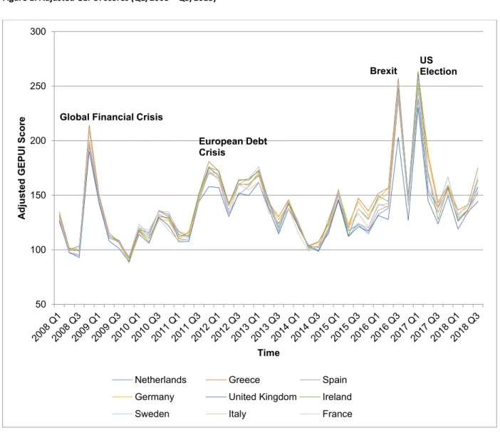
In order to assess the sensitivity of the calculated index optically, Figure 1 displays the development of the adjusted GEPUI across time for the European countries of the data set:

Figure 1: Adjusted GEPUI scores (Q1/2008 – Q3/2018)

Source: Own presentation.

2 The exact econometric specification can be found below in the section “methodology”.

50 100 150 200 250 300

Adjusted GEPUI Score

Time

Netherlands Greece Spain

Germany United Kingdom Ireland

Sweden Italy France

Global Financial Crisis

European Debt Crisis

Brexit US Election

The adjusted GEPUI clearly shows spikes in phases of prominent recent political events, which are generally associated with periods of increased political uncertainty, like the global financial crisis in 08/09, the European debt crisis in 11/12, the 2016 Brexit referendum and the election of the 45

President of the US. In sum, due to the extensive coverage of global economic output and clear measurement of political turmoil, the DEPUI and the adjusted GEPUI both appear to be legitimate proxies for DEPU and GEPU.

2.4 Data and descriptive statistics

The panel data covers observations from 20 European cities (n = 20) in 9 countries [2], with quarterly observations for office properties from Q1/08 to Q3/18 (t = 43). The limiting factor for including markets in the data set is the availability of the DEPUI, which needs to be observable for each market in each period.

On the dependent side, total returns represent the variable of interest, because they are a classic and well-known proxy for property investment performance. The total returns were obtained from CoStar.

The named data provider aggregated the returns from cash-flows as well as from a repeated-sale regression model, which accounts for potential autocorrelation of the data. In order to isolate the impact of the DEPU and GEPU on the direct total returns of direct real estate investments in Europe, the literature review provides the foundation for the variable selection process of the controls. Here, the empirically proven macroeconomic and real-estate-market-related variables were taken from the literature for similar markets and data sets, in order to construct a robust set of control variables to model the remaining variance of the total returns. The variable selection process needs to be conducted particularly carefully, because macroeconomic models are particularly prone to multicollinearity (see Table 1):

Table 1: Data description and variable selection for total return models

Variable Description Proxy for Level Source

Total return The total returns represent the overall appreciation and income return generation of direct real estate investments, as previously used by Akinsomi et al. (2018).

Property Returns

City CoStar

GDP growth Among others, Kohlert (2010) or Akinsomi et al. (2018) argue that the GDP is the most dominant indicator of macroeconomic stability of the direct environment and returns. Hence, the models control for economic output by including quarter-on-quarter GDP growth.

Economic stability

Country OECD

CPI growth Inflation is included in order to control for price Asset price Country OECD

18

noted by e.g. Bond & Seiler (1998) or Brooks & Tsolacos (1999).

Unemployment rate

Employment is often perceived as another indicator of economic health and success. E.g. Liang & McIntosh (1998) use the proxy to isolate the effect of labour- market-related return generation.

Labor market and income

Country OECD

Gov. bond (10 year maturity)

In line with previous literature (e.g. Macgregor &

Schwann, 2003; Baum, 2015), the government bond as an indicator of the overall interest level of other investments is incorporated.

Investment environment

Country OECD

Economic Sentiment Index

In order to distinguish between economic sentiment and EPU, a proxy for the former is introduced (e.g. Tsolacos et al., 2014; Ling et al., 2015). Only by doing so, can the impact of EPU be isolated from the overall economic sentiment.

Economic sentiment

Country Eurostat

Vacancy Office vacancy serves as an indication of the current state of demand in a real estate market, so as to isolate the impact of the markets’ demand side (e.g. in line with De Wit & Van Dijk, 2003; Akinsomi et al., 2018).

Office demand City CoStar

Stock Stock indicates the available office floor space and therefore shows the size of the market and / or the building activity. It is supposed to control for the office supply, in line with West & Worthington (2006).

Office supply

City CoStar

Rent growth Year-on-year rent growth shows the income growth potential of office buildings in the respective market, as proposed by Clayton et al. (2009).

Income expectations

City CoStar

Source: Own presentation.

Based on this selection of variables, the subsequent univariate analysis provides descriptive information about the data. Firstly, since panel data models may be subject to potential non- stationarity, a unit root test to check for temporal econometric distractions is carried out (see Table 6). The non-stationary covariates were differenced, in order to generate a stationary time series, denoted by ∆(x). Table 2 displays the descriptive statistics for both dependent and independent variables, including the target variables:

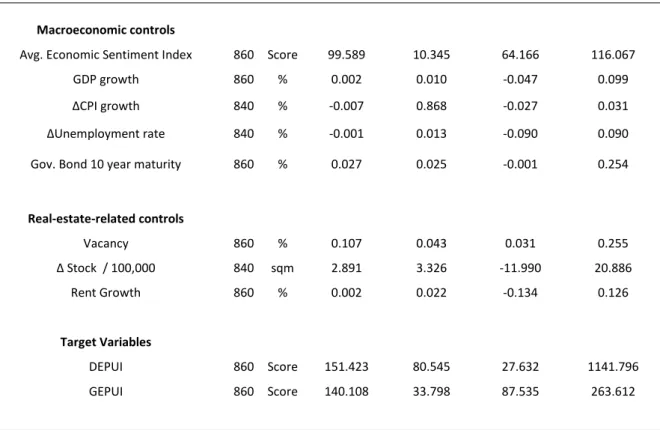
Table 2: Descriptive statistics for variables of the total return models

Variable n Unit Mean SD Min. Max.

Dependent Variable

Total return 860 % 0.016 0.021 -0.092 0.114

Macroeconomic controls

Avg. Economic Sentiment Index 860 Score 99.589 10.345 64.166 116.067

GDP growth 860 % 0.002 0.010 -0.047 0.099

∆CPI growth 840 % -0.007 0.868 -0.027 0.031

∆Unemployment rate 840 % -0.001 0.013 -0.090 0.090

Gov. Bond 10 year maturity 860 % 0.027 0.025 -0.001 0.254

Real-estate-related controls

Vacancy 860 % 0.107 0.043 0.031 0.255

∆ Stock / 100,000 840 sqm 2.891 3.326 -11.990 20.886

Rent Growth 860 % 0.002 0.022 -0.134 0.126

Target Variables

DEPUI 860 Score 151.423 80.545 27.632 1141.796

GEPUI 860 Score 140.108 33.798 87.535 263.612

Note: ∆ indicates the first differences of the variable. Thus, these variables contain one observation less per individual. Sqm stands for square meters.

Source: Own presentation.

From the descriptive statistics table, the need for a natural logarithm transformation of multiple variables becomes apparent, because they differ substantially with regard to their absolute values.

These variables include the target variables and the economic sentiment indicator. The study incorporates all monetary values in Euros to ensure a consistent currency base across all values in the dataset. In addition to the univariate description of the data set, the correlation matrix is reported below (see Table 3):

Table 3: Correlation matrix of the total return data set

1 2 3 4 5 6 7 8 9 10 11

1 Total Return 1.000

2 GDP growth 0.385 1.000

3 ∆CPI growth 0.050 0.053 1.000

4 ∆Unemployment rate 0.044 0.073 0.021 1.000

5 Gov. bond -0.456 -0.338 -0.025 -0.148 1.000

6 Economic Sentiment Index 0.662 0.543 0.176 0.023 -0.532 1.000

7 Vacancy -0.211 -0.024 -0.086 -0.280 0.451 -0.212 1.000

8 ∆Stock 0.020 0.009 -0.013 0.144 -0.151 0.005 -0.291 1.000

9 Rent growth 0.438 0.128 0.027 0.039 -0.172 0.308 -0.171 0.047 1.000

10 DEPUI 0.131 -0.026 -0.069 0.041 -0.173 0.018 -0.278 0.403 0.039 1.000

11 GEPUI 0.119 -0.144 -0.093 -0.110 -0.154 0.036 -0.048 -0.025 0.036 0.405 1.000

Note: ∆ indicates the first differences of the variable.

20

From the correlation matrix, various insights can be obtained. Most importantly, the matrix displays linear correlations that differ from zero for the dependent variable on one hand and the target variables of interest on the other (DEPUI: 0.131; GEPUI: 0.119). Additionally and from a methodologic point of view, other positive correlation values above 0.25 (in line with e.g. Oertel et al., 2020) are defined as the threshold for econometric issues among the independent controlling covariates to monitor multicollinearity (namely GDP growth, rent growth, vacancy and economic sentiment). Thus, the estimation of a clean relationship between the dependent and the target variable are ensured.

Nonetheless, it needs to be highlighted, that the target variables potentially yield information and thus reveal a correlation with other macroeconomic controls.

Accordingly, a base model with all variables is estimated, because the variable selection process above suggests the inclusion of all these variables from an economic perspective. However, from an econometric perspective, the variables mentioned above are systematically excluded in order to carry out robustness checks against potential distractions due to the outlined multicollinearity.

2.5 Methodology

The methodological framework is a classic OLS estimation for the described panel data set. Total returns are the dependent variable, and a multivariate model is specified to estimate the parameters for the covariates:

Total Return_i,t= β_i,t−km_i,t−k+ β_i,t−kr_i,t−k+ β_i,t−kdomestic EPU_i,t−k

+ β_t−kglobal EPU_i,t−k+ β_ttime_t+ β_icity_i+ ε_i,t

(5) Here, the dependent total return observed in a market

abovementioned domestic macroeconomic controls captured in vector m

, and real-estate-related variables in the vector r

. More importantly, the scalars domestic EPU

and global EPU

yield the proxies for the variables of interest:

m_i,t−k= {

ln (Economic Sentiment) GDP growth

∆(CPI growth)

∆(Unemployment rate) Gov. Bond 10 yr maturity

(6)

r_i,t−k= {

Vacancy

∆(Stock) Rent growth

(7)

3 The orthogonalization of the relationship can be an alternative methodological approach to separate the information from the target variable and the control set.

domestic EPUi,t−k= ln (DEPUI)

(8)

(9) Since there may be temporal heterogeneity of returns, dummy variables labeled as time for each year of the sample are incorporated (base = 2008). City heterogeneity is captured throughout all models by including city dummies (as noted by Monfared & Pavlov, 2019). Frankfurt is chosen as the reference, because of its geographic centrality, and ε

represents the error term for each specification.

Furthermore, the relationship between non-fundamentals and direct real estate returns are known for their lagged effects (Case & Shiller, 2003; Case et al., 2014). Accordingly, each model contains lagged terms up to the fourth quarter for the covariates (k = 4, in line with Antonakakis et al., 2015).

An additional remark needs to be made concerning the potential autocorrelation of the dependent variable. In order to account for potential autocorrelation, literature has repeatedly used vector autoregressive models (e.g. Clayton et al., 2009). However, since the present study uses a ML-based OLS estimation in line with Akinsomi et al. (2018), it needs to be highlighted, that the data uses transaction-based capital value returns. In contrast to appraisal-based appreciation, these returns generally do not suffer from appraisal smoothing due to anchoring (in line with Geltner et al., 2003).

Therefore, no autoregressive component is added.

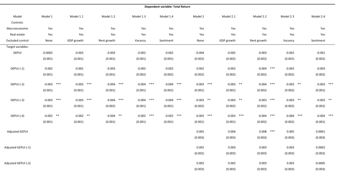
2.6 Empirical results

The results for the OLS models can be found below (see Table 4). The base model in the first column includes all control variables, which were identified above in related studies as important determinants of the total returns. The subsequent models individually exclude the variables of GDP growth, rent growth, vacancy and the economic sentiment index, so as to check for econometric robustness of the beta coefficients of the target variables. The specified variables were systematically exchanged, due to the reported correlation findings. From an economic point of view, the first column displays the central and most important econometric models, containing all relevant controls. Subsequent models are used to conduct various robustness checks.

The models 2.x are specified to assess the second hypothesis regarding the impact of the GEPU. Here,

the DEPUI scores are considered to be part of the control variables in addition to the remaining controls

of the base model specification. The models are then extended by the adjusted GEPUI scores.

22

Table 4: Pooled OLS estimation results (total return)

Dependent variable: Total Return

Model Model 1 Model 1.1 Model 1.2 Model 1.3 Model 1.4 Model 2 Model 2.1 Model 2.2 Model 2.3 Model 2.4

Controls:

Macroeconomic Yes Yes Yes Yes Yes Yes Yes Yes Yes Yes

Real estate Yes Yes Yes Yes Yes Yes Yes Yes Yes Yes

Excluded control None GDP growth Rent growth Vacancy Sentiment None GDP growth Rent growth Vacancy Sentiment

Target variables:

DEPUI -0.0002 -0.003 -0.003 -0.002 -0.002 -0.004 -0.005 -0.003 -0.002 -0.001

(0.001) (0.001) (0.001) (0.001) (0.001) (0.002) (0.002) (0.002) (0.002) (0.002)

DEPUI (-1) -0.002 -0.002 -0.003 -0.002 -0.002 0.002 -0.002 -0.004 *** -0.003 -0.003

(0.001) (0.001) (0.001) (0.002) (0.002) (0.002) (0.002) (0.002) (0.002) (0.002)

DEPUI (-2) -0.003 *** -0.003 *** -0.004 *** -0.004 *** -0.004 *** -0.003 *** -0.003 ** -0.004 *** -0.003 ** -0.003 ***

(0.001) (0.001) (0.001) (0.001) (0.001) (0.001) (0.001) (0.002) (0.002) (0.001)

DEPUI (-3) -0.003 *** -0.003 *** -0.004 *** -0.004 *** -0.004 *** -0.003 ** -0.003 ** -0.003 *** -0.003 ** -0.003 **

(0.001) (0.001) (0.002) (0.001) (0.001) (0.002) (0.002) (0.002) (0.002) (0.002)

DEPUI (-4) -0.002 ** -0.002 ** -0.004 ** -0.002 *** -0.002 *** -0.003 *** -0.003 *** -0.004 *** -0.004 *** -0.004 ***

(0.001) (0.001) (0.001) (0.001) (0.001) (0.001) (0.001) (0.002) (0.002) (0.001)

Adjusted GEPUI 0.005 0.004 0.008 *** 0.005 0.0001

(0.003) (0.003) (0.003) (0.003) (0.003)

Adjusted GEPUI (-1) 0.002 0.003 0.003 0.003 0.0002

(0.002) (0.003) (0.003) (0.003) (0.002)

Adjusted GEPUI (-2) 0.002 0.002 0.003 0.003 -0.0005

(0.003) (0.003) (0.003) (0.003) (0.003)

(0.003) (0.003) (0.003) (0.003) (0.003)

Adjusted GEPUI (-4) 0.008 *** 0.008 *** 0.010 *** 0.010 ** 0.008 ***

(0.003) (0.003) (0.003) (0.003) (0.003)

Time dummies Yes Yes Yes Yes Yes Yes Yes Yes Yes Yes

City dummies Yes Yes Yes Yes Yes Yes Yes Yes Yes Yes

Constant -0.140 *** -0.099 *** -0.303 *** 0.090 *** -0.009 *** -0.276 *** -0.238 *** -0.490 *** -0.368 *** 0.031

(0.056) (0.049) (0.065) (0.014) (0.014) (0.075) (0.067) (0.082) (0.079) (0.036)

Observations 760 760 760 760 760 760 760 760 760 760

Adjusted R² 0.766 0.764 0.702 0.722 0.753 0.767 0.767 0.707 0.726 0.755

Notes: The estimations are based on pooled OLS panel regressions with year and city dummies. “(-t)” denotes the t-th lag of the covariate. The estimation results of the control variables are available upon request. Dummies are included but not reported.

Heteroscedasticity and autocorrelation-robust standard errors were used. ***, ** and * represent statistical significance at 0.01, 0.05 and 0.10 levels, respectively. Standard errors are displayed in parentheses.

Source: Own presentation.

24

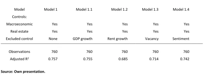
With regard to the overall explanatory power of the econometric models, the results generally yield adjusted R² values around 0.75 – 0.80 for the total returns, which are in line with those in the literature (e.g. recently from Akinsomi et al., 2018). The potential threat of omitted variable bias is sufficiently accounted for, because the explanatory power of the models of the present study yields similar results to existing equivalent studies. Heavy distractions from omitted variables in the control variable set are unlikely to be present. The incremental value of the newly added variables cannot be extracted directly from Table 4. Therefore the same models as above are estimated, but without the DEPUI and GEPUI variables. By doing so, it is possible to show differences in explanatory power of the models without the targets and thus show the incremental value of the newly added target variables (see Table 5):

Table 5: Explanatory power of total return models without DEPUI / GEPUI

Model Model 1 Model 1.1 Model 1.2 Model 1.3 Model 1.4

Controls:

Macroeconomic Yes Yes Yes Yes Yes

Real estate Yes Yes Yes Yes Yes

Excluded control None GDP growth Rent growth Vacancy Sentiment

Observations 760 760 760 760 760

Adjusted R² 0.757 0.755 0.685 0.714 0.742

Source: Own presentation.

As displayed on Table 5, the explanatory power of the models without the DEPUI and the GEPUI reveal lower adjusted R² values for all specifications in comparison to the models reported above. Thus, the introduction of the DEPUI provides an initial value in explanatory power for the modelling of total returns. Since the explanatory power of the models with the GEPUI is again higher than the models including only the DEPUI, the incremental value for both variables can be confirmed (see Table 4).

However, the deltas of the explanatory power values between the models, including the GEPUI proxy and those excluding the specified variable are limited. Thus, general statistical significance can be observed, whereas the low explanatory power of the GEPUI proxy needs to be acknowledged.

Turning to the individual coefficients, the empirical results show c.p. on average a statistically significant negative impact of all lags between the second and fourth period on the DEPUI and the total returns across all specifications. The beta coefficients for the DEPUI reveal a range between -0.003 and -0.004. Since the target variables are transformed by a natural logarithm and the index is denoted in a

4 Estimates for the beta coefficients are explicitly not reported, because these are of minor interest only. In order to isolate the incremental value of the estimates for the DEPUI and GEPUI, however, the explanatory power of the models is sufficient.