Occurrence and characteristics of mesoscale eddies in the tropical northeastern Atlantic Ocean

www.ocean-sci.net/12/663/2016/

doi:10.5194/os-12-663-2016

© Author(s) 2016. CC Attribution 3.0 License.

Occurrence and characteristics of mesoscale eddies in the tropical northeastern Atlantic Ocean

Florian Schütte¹, Peter Brandt^1,2, and Johannes Karstensen¹

1GEOMAR Helmholtz Centre for Ocean Research Kiel, Kiel, Germany

2Christian-Albrechts-Universität zu Kiel, Kiel, Germany Correspondence to: Florian Schütte (fschuette@geomar.de)

Received: 6 November 2015 – Published in Ocean Sci. Discuss.: 18 December 2015 Revised: 26 April 2016 – Accepted: 27 April 2016 – Published: 13 May 2016

Abstract. Coherent mesoscale features (referred to here as eddies) in the tropical northeastern Atlantic Ocean (be- tween 12–22^◦N and 15–26^◦W) are examined and charac- terized. The eddies’ surface signatures are investigated us- ing 19 years of satellite-derived sea level anomaly (SLA) data. Two automated detection methods are applied, the ge- ometrical method based on closed streamlines around eddy cores, and the Okubo–Weiß method based on the relation between vorticity and strain. Both methods give similar re- sults. Mean eddy surface signatures of SLA, sea surface tem- perature (SST) and sea surface salinity (SSS) anomalies are obtained from composites of all snapshots around identified eddy cores. Anticyclones/cyclones are identified by an el- evation/depression of SLA and enhanced/reduced SST and SSS in their cores. However, about 20 % of all anticycloni- cally rotating eddies show reduced SST and reduced SSS instead. These kind of eddies are classified as anticyclonic mode-water eddies (ACMEs). About 146±4 eddies per year with a minimum lifetime of 7 days are identified (52 % cy- clones, 39 % anticyclones, 9 % ACMEs) with rather simi- lar mean radii of about 56±12 km. Based on concurrent in situ temperature and salinity profiles (from Argo float, shipboard, and mooring data) taken inside of eddies, distinct mean vertical structures of the three eddy types are deter- mined. Most eddies are generated preferentially in boreal summer and along the West African coast at three distinct coastal headland regions and carry South Atlantic Central Water supplied by the northward flow within the Mauretanian coastal current system. Westward eddy propagation (on av- erage about 3.00±2.15 km d⁻¹)is confined to distinct zonal corridors with a small meridional deflection dependent on the eddy type (anticyclones – equatorward, cyclones – pole-

ward, ACMEs – no deflection). Heat and salt fluxes out of the coastal region and across the Cape Verde Frontal Zone, which separates the shadow zone from the ventilated sub- tropical gyre, are calculated.

1 Introduction

The generation of eddies in coastal upwelling regions is strongly related to the eastern boundary circulation and its seasonal variations. Within the tropical Atlantic Ocean off northwestern Africa (TANWA; 12 to 22^◦N and 26 to 15^◦W), the large-scale surface circulation responds to the seasonal variability of the trade winds and the north–south migration of the Intertropical Convergence Zone (ITCZ) (e.g., Stramma and Isemer, 1988; Siedler et al., 1992; Stramma and Schott, 1999). The seasonal wind pattern results in a strong seasonal- ity of the flow field along the northwestern African coast and in coastal upwelling of different intensity. The coastal up- welling in the TANWA is mainly supplied by water masses of South Atlantic origin (Jones and Folkard, 1970; Hughes and Burton, 1974; Wooster et al., 1976; Mittelstaedt, 1991; Ould- Dedah et al., 1999; Pastor et al., 2008; Glessmer et al., 2009;

Peña-Izquierdo et al., 2015), which are relatively cold and fresh compared to the North Atlantic waters further offshore.

The water mass transition region coincides with the eastern boundary shadow zone, where diffusive transport pathways dominate (Luyten et al., 1983) with weak zonal current bands superimposed (Brandt et al., 2015). The oceanic circulation in the TANWA is most of the time weak and the velocity field is dominated by cyclonic and anticyclonic eddies. How- ever, global as well as regional satellite-based studies of eddy

distribution and characterization (Chelton et al., 2007, 2011;

Chaigneau et al., 2009) found high eddy activity in terms of eddy generation in the TANWA, but only rare occurrence of long-lived eddies (> 112 days referred to Chelton et al., 2007,

> 35 days, referred to Chaigneau et al., 2009). Karstensen et al. (2015) studied individual energetic eddy events based on a combination of in situ and satellite-based sea level anomaly (SLA) data, and reported eddy life times of more than 200 days in the TANWA region. These individual eddies car- ried water mass characteristics typical for the shelf region up to 900 km off the African coast. One possible genera- tion area for such eddies is the Cap-Vert headland at about 14.7^◦N near the Senegalese coast (Karstensen et al., 2015).

Analyzing surface drifter data and high-resolution satellite data, Alpers et al. (2013) described the evolution of an ener- getic sub-mesoscale eddy at the Cap-Vert headland that was presumably generated by flow separation of a wind-forced coastal jet. Earlier studies reported on the importance of eddy transport in the TANWA region (e.g., Hagen, 1985; Barton, 1987; Zenk et al., 1991). However, characteristics of the eddy field in the TANWA region such as seasonality in eddy gen- eration, eddy lifetime, vertical structure, or frequency of oc- currence are so far undocumented.

More comprehensive information on eddy dynamics was gained for the Pacific Ocean eastern boundary upwelling sys- tems. The eddy generation in the northeastern Pacific Ocean, off California and Mexico including the California Current System, was studied with high-resolution models applied to reproduce observed characteristics of the eddy field (Liang et al., 2012; Chang et al., 2012). These studies not only highlight hotspots of eddy generation associated with lo- cal wind fluctuations (e.g., over the Gulf of Tehuantepec and Papagayo), but also suggest an important role of low- frequency wind and boundary forcing. For the southeastern Pacific Ocean, off Peru and Chile, including the Peru–Chile Current System, Chaigneau et al. (2008, 2011) analyzed the seasonal to interannual variability of eddy occurrence as well as the mean vertical structure of eddies based on Argo floats.

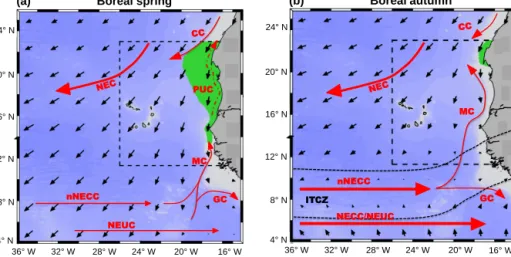
A schematic of the current system of the TANWA in bo- real spring and in boreal autumn is presented in Fig. 1. In the north of the TANWA the Canary Current (CC) transports cold water southwards along the African shelf. It detaches from the coast around Cap Blanc (more specifically at about 20^◦N during spring and 25^◦N during autumn) and joins the North Equatorial Current (NEC) (Mittelstaedt, 1983, 1991).

The dominant feature south of the TANWA is the eastward flowing North Equatorial Countercurrent (NECC) extending over a latitudinal range from 3^◦N to about 10^◦N. It has a pronounced seasonal cycle with maximum strength in bo- real summer and autumn, when the ITCZ reaches its north- ernmost position. During that period the NECC is a con- tinuous zonal flow across the entire tropical Atlantic (e.g., Garzoli and Katz, 1983; Richardson and Reverdin, 1987;

Stramma and Siedler, 1988; Polonsky and Artamonov, 1997).

When approaching the African coast, the current is partly de-

flected to the north feeding a sluggish northward flow along the coast. This current is referred to as Mauretania Current (MC) and reaches latitudes up to 20^◦N (Mittelstaedt, 1991).

The strength of the MC is strongly related to the seasonally varying NECC with a time lag of 1 month (Lázaro et al., 2005). During boreal winter and spring when the NECC is pushed to the Equator and becomes unstable, the MC be- comes weak and unsteady and only reaches latitudes south of Cap-Vert (Mittelstaedt, 1991; Lázaro et al., 2005). During this period the wind induced coastal upwelling is at its max- imum. Simultaneously, the large-scale pressure gradient set by the southward winds induces an along-slope subsurface current, known as Poleward Undercurrent (PUC) (Barton, 1989). During boreal summer the MC re-establishes contem- poraneously to the suppression of coastal upwelling south of Cap Blanc at 21^◦N (Peña-Izquierdo et al., 2012).

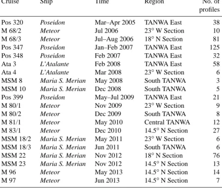
The eastern boundary upwelling is supplied by waters of South Atlantic origin through a pathway consisting of the North Brazil Current (NBC), the North Equatorial Undercur- rent (NEUC) and the PUC. Hence, the purest South Atlantic Central Water (SACW) within the TANWA is found close to the coast (Fig. 2), while further offshore a transition towards the more saline and warmer North Atlantic Central Water (NACW) is observed. The boundary between the regimes is associated with the Cape Verde Frontal Zone (CVFZ; Fig. 2), characterized by a sharp horizontal salinity gradient of 0.9 per 10 km (Zenk et al., 1991). In this study, salinities are reported dimensionless, defined by the UNESCO Practical Salinity Scale of 1978 (PSS-78). The efficiency of mesoscale eddies to transport cold and less saline SACW from their generation regions near the coast into the open ocean where NACW dominates is one topic investigated in this paper. In particular, the characteristics of these eddies (size, structure, frequency) and their potential role in the transport of heat and salt will be examined in more detail.

The paper is organized as follows: in Sect. 2, the different data types (satellite derived and in situ) will be introduced as well as the techniques to automatically detect and track ed- dies from satellite data and to derive their vertical structure.

In Sect. 3 the eddy characteristics (origin, pathways, sur- face signature) and statistics (frequency) are discussed and the temporal and spatial variability of eddy generation and eddy pathways are examined. The mean horizontal and ver- tical eddy structures are derived and, in combination with the eddy statistics, used to estimate the transport of volume, heat, and salt from the shelf region into the open ocean. Finally our results are summarized in Sect. 4.

nNECC

CC

MC GC NEC PUC

NEUC

(a) Boreal spring

24° N

20° N

16° N

12° N

8° N

20° W 24° W 28° W 32° W 36° W

ITCZ nNECC

NEC

CC

MC

GC NECC/NEUC

24° N

16° W 20° N

16° N

12° N

8° N

4° N

20° W 24° W 28° W 32° W 36° W

(b) Boreal autumn

4° N

16° W

Figure 1. Schematic of the current system of the eastern tropical North Atlantic (red arrows; North Equatorial Current (NEC), Canary Current (CC), Poleward Undercurrent (PUC), Mauretania Current (MC), North Equatorial Countercurrent (NECC), Guinea Current (GC), North Equatorial Undercurrent (NEUC)) (a) in boreal spring and (b) in boreal autumn. Black arrows are mean wind vectors, green areas indicate seasonal mean SST < 21^◦C. Blue colors represent topography and the dashed box indicates the TANWA area. The mean position of the Intertropical Convergence Zone (ITCZ) in autumn is indicated as the region bounded by the two black dashed lines in (b).

26 W 24 W 22 W 20 W 18 W 16 W ^{o o o o o o} 35.8 36 36.2 36.4 36.6 36.8

Coastal box: 173 profiles Offshore box: 296 profiles

12 ^oN 14 N ^o 16 N ^o 18 N ^o 20 N ^o 22 N ^o

° C 14 15 16 17 18 19 20

35 35.5 36 36.5 37

8 10 12 14 16 18 20 22 24

25

25

26

26

26

27

27

27

28

28

Salinity

Potential temperature

22° N

20° N

18° N

16° N

14° N

12° N

(a)

(b)

(c)

CVFZ CVOO

NACW

SACW

NACW SACW

26 W 24 W 22 W 20 W 18 W 16 W ^{o o o o o o}

Figure 2. Mean salinity (a) and potential temperature (b) at 100 m depth in the TANWA from the monthly, isopycnal/mixed-layer ocean (MIMOC) climatology (Schmidtko et al., 2013) andθ/Sdiagram (c). The thick black/white line in (a) and (b) indicates the CVFZ. In (a) crosses and dots represent all available profiles (from Argo floats and ships) in the marked coastal and offshore boxes, respectively. In (c), the thin dashed line mark cruise tracks of 20 research cruises to the TANWA taking profiles used in the present study. The black cross in (b) indicates the position of the Cape Verde Ocean Observatory (CVOO) mooring. In (c) data from the coastal and offshore boxes are marked by crosses and dots, respectively; superimposed are isolines of potential density.

2 Data and methods 2.1 Satellite data 2.1.1 SLA, SST, and SSS

The delayed-time reference data set “all-sat-merged” of SLA (Version 2014), which is used in the study, is produced by Ssalto/Duacs and distributed by AVISO (Archiving, Vali- dation, and Interpretation of Satellite Oceanographic), with support from CNES (http://www.aviso.altimetry.fr/duac/).

The data are a multi-mission product, mapped on a 1/4^◦× 1/4^◦Cartesian grid and has a daily temporal resolution. The anomalies are computed with respect to a 20-year mean. Data for the period January 1995 to December 2013 are consid- ered here. Geostrophic velocity anomalies derived from the SLA provided by AVISO for the same timespan are also used in this study. Given the interpolation technique applied to the along track SLA data Gaussian shaped eddies with a ra- dius >∼45 km can be detected; eddies of smaller diameter may be detected but their energy is damped (Fu and Ferrari, 2008).

For sea surface temperature (SST) the data set “Microwave Optimally interpolated Sea Surface Temperature” from Re- mote Sensing Systems (www.remss.com) is used. It is de- rived from satellite microwave radiometers, which have the capability to measure through clouds. It has a 25 km resolu- tion and contains the SST measurements from all operational radiometers for a given day. All SST values are corrected us- ing a diurnal model to create a foundation SST that represents a 12:00 LT temperature (www.remss.com). Daily data from the outset (1 January 1998 to 31 December 2013) are used here and mapped similar to the SLA data on a 1/4^◦×1/4^◦ Cartesian grid.

Our study also includes sea surface salinity (SSS) data.

We make use of the LOCEAN_v2013 SSS product avail- able from 1 January 2010 until the end of our analysis period (31 December 2013). The data are distributed by the Ocean Salinity Expertise Center (CECOS) of the Centre National d’Etudes Spatiales (CNES) – Institut Français de Recherche pour l’Exploitation de la Mer (IFREMER) Centre Aval de Traitemenent des Donnees SMOS (CATDS), at IFREMER, Plouzane (France). The data are created using the weight av- eraging method described in Yin et al. (2012) and the flag sorting described in Boutin et al. (2013). Finally the data are mapped on a 1/4^◦×1/4^◦Cartesian grid and consist of 10- day composites.

2.1.2 Eddy identification and tracking from satellite data

In order to detect eddy-like structures, two different meth- ods are applied to the SLA data. The first method, the Okubo–Weiß method (OW method; Okubo, 1970; Weiss, 1991), has been frequently used to detect eddies using satel-

lite data as well as the output from numerical studies (e.g., Isern-Fontanet et al., 2006; Chelton et al., 2007; Sangrà et al., 2009). The basic assumption behind the OW method is that regions, where the relative vorticity dominates over the strain, i.e., where rotation dominates over deformation, char- acterize an eddy. In order to separate strong eddies from the weak background flow field a threshold needs to be identi- fied. For this study the threshold is set toW₀= −0.2×σ, whereσis the spatial standard derivation of the Okubo–Weiß parameterW=s_n²+s_s²−ω². Here,s_n= ^∂u

∂x−^∂v

∂y is the normal strain,ss= ^∂v

∂x+^∂u

∂y is the shear strain andω= ^∂v

∂x−^∂u

∂y is the relative vorticity. A similar definition of the threshold was used in other eddy studies applying the OW method (e.g., Chelton et al., 2007). The maximum (minimum) SLA marks the eddy center.

The second method for eddy detection is based on a ge- ometric approach (in the following GEO method) analyz- ing the streamlines of the SLA-derived geostrophic flow. An eddy edge is defined as the streamline with the strongest swirl velocity around a center of minimum geostrophic ve- locity (Nencioli et al., 2010). For the detection of an eddy, the algorithm requires two parametersaandbto be defined.

The first parameter,a, is a search radius in grid points. In- side the search radius, the velocity reversal across the eddy center is identified (vcomponent on an east–west section,u component on a north–south section). The second parameter, b, is used to identify the point of minimum velocity within a region that extends up to b grid points (for a more de- tailed description of the method see Nencioli et al., 2010).

After a few sensitivity tests in comparison with the results of the OW method and following the instructions of Nencioli et al. (2010), we seta=3 andb=2. Optimal results were obtained when we linearly interpolated the AVISO velocity fields onto a 1/6^◦×1/6^◦grid before we applied the algorithm (for more information see also Liu et al., 2012). If an eddy is detected, then an eddy center is identified in analogy to the OW method as the maximum (anticyclone) or the minimum (cyclone) of SLA within the identified eddy structure.

When applying the two different eddy detection methods to the SLA data from the TANWA region, we used the same eddy detection thresholds for both methods; i.e., a feature only counts as an eddy, if its radius is larger than 45 km and it is detectable for a period of more than 7 days. Note, as the identified eddy areas are rarely circular we used the circle- equivalent of the area of the detected features to estimate the radius. For eddy tracking both eddy detection methods use the same tracking algorithm. An eddy trajectory was calcu- lated if an eddy with the same polarity was found in at least 7 consecutive SLA maps (corresponding to 1 week) within a search radius of up to 50 km. Due to, e.g., errors in SLA map- pings (insufficient altimetric coverage) an eddy could van- ish and re-emerge after a while. Therefore we searched in 14 consecutive SLA maps (corresponding to 2 weeks) in a search radius of up to 100 km after an eddy disappearance, if

eddies with the same polarity re-emerges. If more than one eddy with the same polarity emerge within the search radius, we defined the following similarity parameter to discriminate between these eddies:

X= s

distance 100

2

+ 1radius

radius₀ 2

+

1vorticity vorticity₀

2

+ 1EKE

EKE₀ 2

, (1)

which include four terms based on the distance between the disappeared and newly emerged eddies and the difference of their radii, mean vorticity, and mean eddy kinetic energy (EKE). Radius0, vorticity0, and EKE0 are the mean radius, vorticity and EKE of all identified eddies in TANWA. The newly emerged eddy with the smallest x is selected to be the same eddy. To give an idea of the uncertainty related to the detection technique, both methods are applied to the data.

Every step is computed separately with both methods and the results are compared.

2.1.3 Eddy classification and associated mean spatial surface pattern

From the geostrophic velocity data, anticyclones (cyclones) can be identified due to their negative (positive) vorticity.

In the SLA data anticyclones (cyclones) are associated with a surface elevation (depression). The maximum (minimum) SLA marks the eddy center. In general, anticyclones (cy- clones) carry enhanced (reduced) SST and enhanced (re- duced) SSS in their cores, respectively. However, we found that 20 % of all detected anticyclones had cold anomalies in their cores and a reduced SSS. This kind of eddies is clas- sified as an anticyclonic mode-water eddy (ACME) or in- trathermocline eddy (Kostianoy and Belkin, 1989) as will later be confirmed when considering the in situ observations (see below). Given that ACMEs show distinct characteristics, which are contrasting to anticyclones (see below), we distin- guish in the following three types of eddies: anticyclones, cyclones, and ACMEs.

Composites of satellite-derived SST and SSS anomalies with an extent of 300 km×300 km around the eddy centers yield the mean spatial eddy surface pattern of temperature and salinity for the respective eddy type. The information whether an eddy is cold/warm or fresh/saline in the core is obtained by subtracting the average value over the edge of the box from the average value over the eddy center and its clos- est neighboring grid points. To exclude large-scale variations in the different data sets, the SST and SSS fields are low-pass filtered with cutoff wavelength of 15^◦longitude and 5^◦lati- tude. Thereafter the filtered data sets are subtracted from the original data sets thus preserving the mesoscale variability.

The composite plots are based only on eddies with a radius between 45 and 70 km and an absolute SLA difference be- tween the eddy center and the mean along the edge of the 300 km×300 km box used for the composites greater than 2 cm.

2.2 In situ data 2.2.1 Argo floats

A set of irregular distributed vertical CTD (conductivity–

temperature–depth) profiles was obtained from the au- tonomous profiling floats of the Argo program. The freely available data were downloaded from the Global Data As- sembly Centre in Brest, France (www.argodatamgt.org) and encompasses the period from July 2002 to December 2013.

Here only pressure (P), temperature (T), and salinity (S) data flagged with Argo quality category 1 are used. The given uncertainties are±2.4 dbar for pressure,±0.002^◦C for tem- perature, and±0.01 for uncorrected salinities. In most cases the salinity errors are further reduced by the delayed-mode correction. For this analysis an additional quality control is applied in order to eliminate spurious profiles and to en- sure good data quality in the upper layers. In the following, we give the criteria applied to the Argo float profiles and in brackets the percentage, to which the criteria were fulfilled.

Selected profiles must (i) include data between 0 and 10 m depth (98.2 %), (ii) have at least 4 data points in the upper 200 m (98.8 %), (iii) reach down to 1000 m depths (95 %), with (iv) continuous and consistent temperature, salinity, and pressure data (78 %). This procedure reduced the number of profiles by around 30 % to 2022 Argo float profiles for the TANWA.

2.2.2 Shipboard measurements

In situ CTD profile data collected during 20 ship expe- ditions to the TANWA within the framework of different programs are used (Fig. 2b; see Table 1 for further de- tails). In total 579 profiles were available taken within the TANWA during the period March 2005 to June 2013. Data sampling and quality control followed the standards set by Global Ocean Ship-Based Hydrographic Investigations Pro- gram (GO-SHIP) (Hood et al., 2010). However, we as- sume a more conservative accuracy of our shipboard data of about twice the GO-SHIP standard, which is±0.002^◦C and

±0.004 for temperature and salinity, respectively.

2.2.3 CVOO mooring

The third set of in situ data stems from the Cape Verde Ocean Observatory (CVOO) mooring. The CVOO moor- ing is a deep-sea mooring deployed at a depth of about 3600 m, 60 km northeast of the Cabo Verdean island of São Vicente (Fig. 2b). The nominal mooring position is 17^◦36⁰N, 24^◦15⁰W. The mooring was first deployed in June 2006 and has been redeployed in March 2008, October 2009, May 2011, and October 2012. Temperature and salinity mea- surements in the upper 400 m have been typically recorded at depth of 30, 50, 70, 100, 120, 200, 300, and 400 m using MicroCAT instruments. Data calibration is done against ship-

Table 1. Data from the following research cruises were used.

Cruise Ship Time Region No. of

profiles

Pos 320 Poseidon Mar–Apr 2005 TANWA East 38

M 68/2 Meteor Jul 2006 23^◦W Section 10

M 68/3 Meteor Jul–Aug 2006 18^◦N Section 81

Pos 347 Poseidon Jan–Feb 2007 TANWA East 125

Pos 348 Poseidon Feb 2007 TANWA East 32

Ata 3 L’Atalante Feb 2008 TANWA East 58

Ata 4 L’Atalante Mar 2008 23^◦W Section 6

MSM 8 Maria S. Merian May 2008 South TANWA 3

MSM 10 Maria S. Merian Dec 2008 South TANWA 5

Pos 399 Poseidon May–Jul 2009 TANWA East 21

M 80/1 Meteor Nov 2009 23^◦W Section 9

M 80/2 Meteor Dec 2009 South TANWA 8

M 81/1 Meteor May 2010 Central TANWA 12

M 83/1 Meteor Dec 2010 14.5^◦N Section 27

MSM 18/2 Maria S. Merian May 2011 23^◦W Section 6

MSM 18/3 Maria S. Merian Jun 2011 South TANWA 6

MSM 22 Maria S. Merian Nov 2012 18^◦N Section 76

MSM 23 Maria S. Merian Nov 2012 14.5^◦N Section 13

M 96 Meteor May 2013 14.5^◦N Section 14

M 97 Meteor Jun 2013 14.5^◦N Section 7

P557

board CTD data during the service cruises. The uncertainties are±0.002^◦C for temperature and±0.01 for salinity.

The eddy detection method identifies 22 eddies passing the CVOO mooring. For these eddy events, the original time series with a temporal resolution of 15 or 20 min were low- pass filtered with a cutoff period of 24 h and consecutively subsampled to 1-day values in order to reduce instrument noise and to match the resolution of the SLA maps. In to- tal 429 profiles could be obtained.T /S(temperature/salinity) anomaly profiles were derived as the difference of profiles inside and outside of the eddies. The outside profiles were taken shortly before the eddy passage.

2.3 Determining the vertical structure of eddies detected in SLA data

In order to investigate the vertical structure of eddies identi- fied in SLA data, a combination of all available in situ data sets was used. We had a total of 3030 CTD profiles available for the time period 2002 to 2013, with about 67 % Argo float profiles, 19 % shipboard CTD profiles, and 14 % mooring- based profiles (Fig. 3). All profiles were vertically interpo- lated or re-gridded to 1 m vertical resolution in the depth range 5 to 1000 m. Missing data points within the first few meters of the water column were filled by constant extrapo- lation. For each profile, we determined the mixed layer depth (MLD) as the depth where the in situ temperature decreased by 0.2^◦C relative to 10m depth (de Boyer Montégut et al., 2004).

22 ° N

14 ° N

26° W 16° W

16 ° N 18 ° N 20 ° N

24° W 22° W 20° W 18° W

Figure 3. Locations of available temperature and salinity profiles obtained in the TANWA between 1995 and 2013. Red dots mark shipboard CTD stations, blue dots locations of Argo float profiles, and the black cross the location of the CVOO mooring.

By co-location, in space and time, of eddies, which are identified in the SLA data using a combination of the OW and the GEO method (an eddy has to be identified by both algorithms), with the combined in situ data set, the vertical structures of anticyclones and ACMEs (positive SLA) and cyclones (negative SLA) were assessed (Fig. 4). The classi- fication results in 675 profiles taken in anticyclones/ACMEs, 499 profiles taken in cyclones, and 1856 profiles taken out- side of detected eddies. Excluding the mooring-based pro-

24^oW 22^o 20^oW 18^o W 16^oW 12^oN

14^oN 16^oN 18^oN 20^oN 22^oN

CVOO

Okubo−Weiß Geometric Method

CVOO

Okubo−Weiß Geometric Method 22. Dec. 2010

SLA (cm)²

4 6 8 10 12 14

24^{o o} 20^o 18^o 16^oW 12^oN

14^oN 16^oN 18^oN 20^oN 22^oN

CVOO

Okubo−Weiß Geometric Method 22. Dec. 2010

SLA (cm)²

4 6 8 10 12 14

21^oW ^30’ 20^oW ^30’ 19^oW ^30’ 18^oW

19^oN 20’

40’

20^oN 20’

40’

21^oN

(b) (a)

6

4

2

0

-2

-4

-6

SLA [cm]

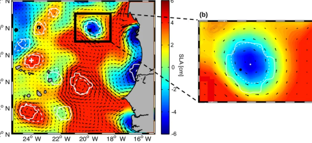
W

Figure 4. Snapshot of the SLA for 22 December 2010, with the results of the eddy-detection methods: OW method (solid white line) and the GEO method (dashed white line) with geostrophic velocities superimposed (black arrows). The black dots mark Argo float profiles, the white cross in (a) indicates the CVOO mooring. In (b) a zoom of a selected region with a cyclonic eddy is shown.

files, from which we only extracted eddy events, around

∼29 % of all profiles (Argo float and shipboard CTD pro- files) were taken coincidentally inside of an eddy. This pro- portion is in the range of earlier results derived by Chaigneau et al. (2011), who estimated that ∼23 % of their Argo float profiles in the eastern upwelling regions of the Pacific Ocean are conducted in eddies and Pegliasco et al. (2015), who found 38 % of all their Argo float profiles in the eastern up- welling areas conducted in eddies. We could also confirm with the result of Pegliasco et al. (2015) that the majority of all Argo float profile in eddies are conducted in long-lived anticyclones/ACMEs.

However, we are interested in the anomalous water mass characteristic inside the eddy compared to the surrounding water. Anomaly profiles of potential temperature,θ, salinity, S, and potential density,σ_θ, were derived as the difference of the profiles inside and reference profiles outside of an eddy.

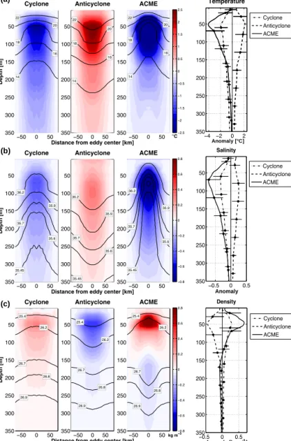
Profiles outside of eddies are required to be taken within a maximum distance of 120 km from the eddy center and at maximum±25 days apart from the time the profile inside of the eddy was taken (Fig. 4). For 176 profiles out of the 1174 profiles inside of eddies, no reference profile could be found fulfilling these criteria. In total 587 anomaly profiles for an- ticyclones/ACMEs and 411 anomaly profiles for cyclones were derived. As mentioned before it was useful to further separate anticyclonically rotating eddies into two types: con- ventional anticyclones with downward bending isopycnals (and isotherms) throughout and ACMEs with upward bend- ing isopycnals in the upper 50 to 100 m depth and downward bending isopycnals below. As a consequence, the MLD in- side the ACMEs is shallower compared to background val- ues, while it can be several tens of meters deeper in conven- tional anticyclones. We used the MLD difference to proof the separation into conventional anticyclones and ACMEs from the satellite-based surface signatures, described above. In all

cases, where the MLD inside of an anticyclonically rotating eddy was at least 10 m shallower than the MLD outside the eddy, the eddy was associated with a negative SST anomaly.

Hence, the eddy-type separation through satellite-based sur- face signatures appears to be accurate. The separation identi- fied 95 out of 587 profiles in anticyclonically rotating eddies as being taken in ACMEs (Fig. 5). Averaging all anomaly profiles for anticyclones, cyclones, and ACMEs yields mean anomaly profiles for potential temperature,θ⁰, salinity, S⁰, and potential density,σ_θ⁰, for the three different eddy types.

Profiles of available heat and salt anomalies available heat anomalies (AHA [J m⁻¹]) and available salt anomalies (ASA [kg m⁻¹]) per meter on the vertical were then derived as

AHA=π r²ρC_pθ⁰, (2)

ASA=0.001×π r²ρS⁰, (3)

whereρ is density (in kg m⁻³), C_p is specific heat capac- ity (4186.8 J kg⁻¹K⁻¹), andris the mean radius. The factor 0.001 in Eq. (2) is an approximation to convert PSS-78 salin- ity to salinity fractions (kg of salt per kg of seawater). These calculations are partly adapted from Chaigneau et al. (2011), where AHA and ASA are computed for eddies in the eastern Pacific. Integrating AHA and ASA per meter over the depth range 0 to 350 m, the AHAtotal(in J) and ASAtotal(in kg) was obtained. The lower boundary of integration was chosen as below; 350 m no significant temperature and salinity anoma- lies could be identified for the composite eddies of the three eddy types.

Eddies that pinch off from the eastern boundary are ex- pected to carry waters with SACW signature westward into areas where waters with NACW signature prevail. To quan- tify the amount of SACW carried by these eddies, we fol- low a method developed by Johns et al. (2003) used to quan- tify the amount of water of Southern Hemisphere origin car- ried by North Brazil Current rings. Accordingly the high-

22° N

18° N

14° N

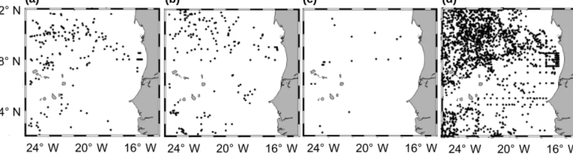
(a) (b) (c) (d)

24° W 20° W 16° W 24° W 20° W 16° W 24° W 20° W 16° W 24° W 20° W 16° W Figure 5. Location of all profiles taken in (a) cyclones, (b) anticyclones, (c) ACMEs, and (d) outside of an eddy.

est/lowest 10 % of the salinity values on potential density surfaces were averaged to define the mean NACW/SACW characteristics in the region as function of potential density.

The obtained characteristics were used to determine the per- centage of SACW contained in any profile taken inside and outside of eddies. Anomaly profiles of SACW percentage as function of potential density were then calculated as the dif- ference of the profiles inside and outside of eddies and were eventually transformed back into depth space using a mean density profile.

To illustrate mean anomalies in potential temperature, salinity, potential density, and SACW percentage for each eddy type as a function of depth and radial distance, the available profiles were sorted with respect to a normalized distance, which is defined as the actual distance of the pro- file from the eddy center divided by the radius of the eddy.

The profiles were grouped and averaged onto a grid of 0.1 between 0 and 1 of the normalized radial distance. Finally, the field was mirrored at zero distance and a running mean over three consecutive horizontal grid points was applied.

2.4 Determining the heat, salt, and volume transport The three-dimensional structures of composite cyclones, an- ticyclones, and ACMEs produced out of the combination of altimetry data and all available profiles were used to estimate the relative eddy contribution to fluxes of heat, salt, and vol- ume in the TANWA. Here we chose to define enclosed areas with area I representing the extended boundary current re- gion, area II the transition zone, and area III the subtropical gyre region. By multiplying the heat transport of the compos- ite eddies with the number of eddies dissolving during a year in a given area (corresponding to an flux divergence) a mean heat release (in W m⁻²)and a mean salt release (in kg m⁻²) were calculated. The mean heat release can be compared to the net atmospheric heat flux in the area here derived from the NOCS Surface Flux Dataset (Berry and Kent, 2011).

Using the volume of a composite eddy (defined by the mean radius and the depth range 0 to 350 m) and the mean SACW percentage within the eddy, the total volume trans- port of SACW of cyclones, anticyclones, and ACMEs was calculated.

ACME Ant Cyc

13 80 07 17 33 50 00 53 47 06 56 38 13 57 30 10 41 48 11 44 45 07 46 46 09 39 52 09 39 52 10 35 55

ACME Ant Cyc

09 74 17 00 20 80 00 53 47 00 53 48 14 47 39 07 43 51 09 32 59 10 40 50 08 44 48 09 40 52 10 39 51

OW-method GEO-method

Number of eddies 0 500 1000 1500 Number of eddies 1500 1000 500 0

>150 135 120

90 75 60 45 30 15 7 105

Cyclones AnFcyclones ACMEs

Figure 6. Number of eddies against lifetime in days from the OW method (left) and GEO method (right). Percentage of ACMEs, an- ticyclones (Ant), and cyclones (Cyc) is given in the tables on the right and left.

3 Results and discussion

3.1 Eddy statistics from SLA data

The two eddy tracking methods applied to the SLA data detected∼2800 eddies over the 19 years of analyzed data (Table 2, Fig. 6) with slightly more cyclones than anticy- clones/ACMEs (6 % more in the OW method, 2 % more in the GEO method). Note, that the given number of eddies must be seen as a lower limit due to the coarse resolution of the satellite products. All of the detected eddies are nonlin- ear by the metricU/c, whereU is the maximum circumpo- lar geostrophic surface velocity and c is the translation speed of the eddy. A value ofU/c>1 implies that fluid is trapped within the eddy interior (Chelton et al., 2011) and exchange with the surrounding waters is reduced. Many of the eddies are even highly nonlinear, with 60 % havingU/c>5 and 4 % havingU/c>10.

Table 2. Mean properties of anticyclones, cyclones, and ACMEs in the region of 12–22^◦N, 16–26^◦W (TANWA) and their standard deviation given in brackets, detected from the OW method and the GEO method (detectable longer than 1 week and with a radius > 45 km). Coastal area is defined as an∼250 km wide corridor near the coast (see Fig. 7).

Property

(based on SLA data between 95–2013)

OW method GEO method

Detected eddies 2741 (144 yr⁻¹) 2816 (148 yr⁻¹)

Anticyclones Cyclones ACMEs^∗ Anticyclones Cyclones ACMEs^∗

1041 (38 %)

1443 (53 %)

257 (9 %)

1137 (40 %)

1422 (51 %)

257 (9 %) Detected eddies

in coastal area

186 (10 yr⁻¹)

241 (13 yr⁻¹)

43 (2 yr⁻¹)

178 (9 yr⁻¹)

199 (10 yr⁻¹)

45 (3 yr⁻¹) Average lifetime (days) 30 (±31)

max 282

24 (±22) max 176

26 (±28) max 197

32 (±32) max 277

27 (±29) max 180

26 (±28) max 175

Average radius (km) 53 (±5) 51 (±5) 52 (±5) 60 (±20) 62 (±22) 59 (±20)

Average westward propagation (km d⁻¹)

2.8 (±2.4) 2.7 (±2.4) 2.8 (±2.5) 3.3 (±1.8) 3.1 (±1.9) 3.3 (±1.9)

∗Note, that the properties of ACMEs are based on fewer years of SLA data (1998–2013), due to the unavailable SST data.

Considering only the period after 1998, i.e., when our SST data set becomes available, a satellite data-based separation between anticyclones (positive SST anomalies) and ACMEs (negative SST anomalies) is possible. We found that about 20 % of the anticyclonically rotating eddies are ACMEs.

However, the number of ACMEs might be underestimated, because ACMEs are associated with a weak SLA signature and therefore more difficult to detect with the SLA-based al- gorithms. Also the nonlinearity of ACMEs is underestimated by using geostrophic surface velocity as they have a subsur- face velocity maximum.

Although the GEO method in general detects slightly more eddies than the OW method (in total 75 eddies more, which is 2.7 % more than the OW method) the situation is different near the coastal area where the OW method detects 30 eddies per year but the GEO method only 22 eddies per year. This results from the strong meandering of the boundary current, where meanders are sometimes interpreted as eddies by the OW method due to the high relative vorticity. In contrast, the GEO method uses closed streamlines and therefore does not detect meanders as eddies, which makes this method more suitable for eddy detection in coastal areas. The average eddy radius in the TANWA is found to be 56±12 km (given here as mean and standard derivation) with the GEO method re- sulting not only in around 10 km larger radii but also with a 4 times higher standard deviation when compared with the OW method. The difference in the standard deviation of the eddy radius derived from GEO and the OW method is partly due to the identification of relatively few very large eddies using the GEO method. In general, the OW method appears to be the more reliable tool for identifying the eddy surface area and the corresponding radius in the TANWA.

Both algorithms show that on average the anticyclones and ACMEs are larger and have a longer lifetime than the cyclones. The average westward propagation speed is 3.00±2.5 km d⁻¹for all eddy types, which is on the order of the first baroclinic mode Rossby wave phase speed at that latitude range (Chelton et al., 1998). The average tracking period (or lifetime) of an eddy in the TANWA is 28 days with a high standard deviation of 28 days. The longest con- secutive tracking period for a single eddy (found similar in both algorithms) was around 280 days for an anticyclone, 180 days for a cyclone and 200 days for an ACME. How- ever, most of the eddies were detectable for a period of 7 to 30 days. The number of eddies decreases rapidly with in- creasing tracking period (Fig. 6). Note that the OW method detects 450 eddies with a lifetime between 7 and 14 days, which is more than the GEO method. However, for longer lifetimes the GEO method detects more eddies than the OW method. As the tracking procedure in both algorithms is the same, the GEO method seems to be more reliable in identi- fying and following eddy-like structures from one time step to another. The percentage of tracked anticyclones/ACMEs and cyclones is close to 50 % for short tracking periods. For longer lifetimes anticyclonic eddies tend to dominate, this is also reflected in the slightly shorter mean lifetimes of cy- clones compared to anticyclones. The dominance of long- lived anticyclones is also shown in the observational studies of Chaigneau et al. (2009), Chelton et al. (2011), and theoret- ically suggested by Cushman-Roisin and Tang (1990). The latter authors showed that in an eddying environment anti- cyclonic eddies are generally more robust and merge more freely than cyclones producing long-lived eddies, while cy- clones show a higher tendency to self-destruction.

Note, that tracking of eddies in the TANWA is prone to errors in particular regarding the information about the ed- dies’ lifetime. Some eddies disappear in single SLA maps, which is at least partly due to the separation of the satellite ground tracks (Chaigneau et al., 2008). In order to avoid loos- ing an eddy, we search 2 weeks after its assumed disappear- ance within a defined radius for an eddy with the same po- larity (see Sect. 2.1.2). The fact that purest SACW, which in the TANWA occurs in the eastern boundary region, is found regularly in eddy cores at the CVOO mooring (∼850 km off- shore) (Karstensen et al., 2015) shows that long-lived eddies must exist in the TANWA. Hence, the eddy tracking algo- rithms underestimate the eddy lifetime and accordingly over- estimate the number of newly generated eddies.

This challenge for the eddy tracking algorithms in the TANWA is probably the reason why Chelton et al. (2011) and Chaigneau et al. (2009) could not detect many long-lived ed- dies in this area. Their definition of long-lived eddies requires eddies to be trackable for longer than 112 days (Chelton et al., 2011) or 35 days (Chaigneau et al., 2009). With the adap- tion of the method for the TANWA with the 2 weeks search radius as described above, eddy tracking has improved; how- ever, some eddies might still be lost. In addition, the mean eddy lifetime of eddies in TANWA is underestimated due to the restriction of eddy trajectories at the northern, southern, and western boundaries.

3.2 Generation areas and pathways

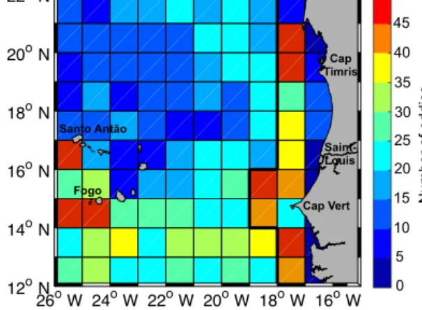
To identify hot spots of eddy generation, the locations of the first detection of each eddy is counted in 1^◦×1^◦boxes (Fig. 7). The OW method and the GEO method do not show a significantly different pattern, except near the coast, where the local maximum in the number of newly detected eddies is shifted slightly offshore for the GEO method compared to the OW method. However, the distribution shows that most ed- dies are generated in the coastal area along the shelf. Within this region the headlands of the coast seem to play an im- portant role as about nine newly detected eddies per year are found around Cap-Vert (Senegal), about four eddies per year off Saint-Louis (Senegal) and about five eddies per year off Cap Timris (Mauretania). At these spots the algorithms de- tect more than 70 % of the newly detected eddies (18 out of 25) per year in the coastal area. Another location of high eddy generation is southeast of the Cabo Verde islands, espe- cially south of the northwesternmost island Santo Antão with about two newly detected eddies per year and southwest of Fogo with about five newly detected eddies per year.

To identify the preferred eddy propagation pathways, the locations of eddy centers, which were tracked for longer than 1 month (35 days), were counted in 1/6^◦×1/6^◦boxes over all time steps. The spatial distribution of eddy activity indeed shows some structures and eddies tend to move along dis- tinct corridors westward, away from the coast into the open ocean (Fig. 8) as also shown for the Canary Island region

26^oW 24^oW 22^oW 20^oW 18^oW 16^oW 12^oN

14^oN 16^oN 18^oN 20^oN 22^oN

Number of Eddies

0 5 10 15 20 25 30 35 40 45 50

Saint- Louis

Cap Vert Cap Timris

Fogo Santo Antão

Number of eddies

50

40

0 45

35 30 25 20 15 10 5

Figure 7. Number of eddies generated in 1^◦×1^◦ boxes (colors) between 1995 and 2013 based on the results of the OW method.

Marked are the headlands Cap Timris (Mauretania), Saint-Louis (Senegal), Cap-Vert (Senegal), and the islands Santo Antão (Cabo Verde) and Fogo (Cabo Verde), which can be associated with high eddy generation. The thick solid black line along 18^◦W/19^◦W sep- arates the coastal region from the offshore region.

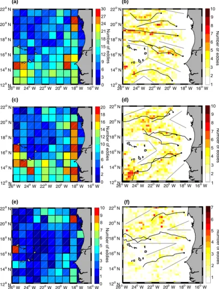
(Sangrà et al., 2009). The propagation pathways can be sep- arately investigated for the different eddy types: most of the anticyclones are generated along the coast south of Cap Tim- ris, off Saint-Louis, and north off Cap-Vert. They propagate either north of 18^◦N from their generation areas westward into the open ocean or south of 18^◦N with a southward de- flection offshore. Their mean westward propagation speed is 3.05±2.15 km d⁻¹. Other generation hotspots for anticy- clones are around the Cabo Verde islands south of Santo Antão and south of Fogo. For cyclones the generation ar- eas are more concentrated than for anticyclones. North of Cap Timris and off Cap-Vert are the main hotspots near the coast. On their way westwards cyclones tend to have a northward deflection in their pathways. The hotspot for cy- clone generation around the Cabo Verde islands is west of Fogo. Cyclones have a mean westward propagation speed of 2.9±2.15 km d⁻¹. Although not significantly different, the larger westward propagation speed of anticyclones com- pared to cyclones does agree with theoretical considerations regarding the westward eddy drift on a beta plane (Cushman- Roisin et al., 1990).

The main generation areas for ACMEs near the coast are north of Cap Timris and off Saint-Louis around 18^◦N.

ACMEs generated north of Cap Timris tend to have a slightly southward deflection on their way westwards into the open ocean, whereas the eddies generated off Saint-Louis show no meridional deflection and propagate along∼18^◦N into the open ocean. Their mean westward propagation speed is 3.05±2.1 km d⁻¹. The main generation area of ACMEs near Cabo Verde islands is located south of the northwesternmost island Santo Antão.

!

Number of Eddies

1 2 3 4 5 6 7 8 9 10

Number of Eddies

1 2 3 4 5 6 7 8 9 10

Number of Eddies

1 2 3 4 5 6 7

26 W 24 W 22 W 20 W 18 W 16 W ^{o o o o o o} 12 ^oN

14 N ^o 16 N ^o 18 N ^o 20 N ^o 22 N ^o

Number of Eddies

0 3 6 9 12 15 18 21 24 27 30

Number of Eddies

0 1 2 3 4 5 6 7 8 9 10

Number of Eddies

0 2 4 6 8 10 12 14 16 18 20

(a)

(c)

(e)

(b)

(d)

Number of Eddies

1 2 3 4 5 6 7

Number of Eddies

1 2 3 4 5 6 7 8 9 10

Number of Eddies

1 2 3 4 5 6 7 8 9 10

Number of eddies

30 27

21 18 15 12 9 6 3 0 24

Number of eddies

20 18

14 12 10 8 6 4 2 0 16

Number of eddies

10 9

7 6 5 4 3 2 1 0 8

Number of eddies

7

5 4 3 2 1 6

Number of eddies

10 9

7

5 6

4 3 2 1 8

Number of eddies

10 9

7

5 6

4 3 2 1 8

( f )

26 W 24 W 22 W 20 W 18 W 16 W ^{o o o o o o} 12 ^oN

14 N ^o 16 N ^o 18 N ^o 20 N ^o 22 N ^o

!

26 W 24 W 22 W 20 W 18 W 16 W ^{o o o o o o} 12 ^oN

14 N ^o 16 N ^o 18 N ^o 20 N ^o 22 N ^o

26 W 24 W 22 W 20 W 18 W 16 W ^{o o o o o o} 12 ^oN

14 N ^o 16 N ^o 18 N ^o 20 N ^o 22 N ^o

!

26 W 24 W 22 W 20 W 18 W 16 W ^{o o o o o o} 12 ^oN

14 N ^o 16 N ^o 18 N ^o 20 N ^o 22 N ^o

26 W 24 W 22 W 20 W 18 W 16 W ^{o o o o o o} 12 ^oN

14 N ^o 16 N ^o 18 N ^o 20 N ^o 22 N ^o

Figure 8. Number of eddies generated in 1^◦×1^◦boxes (a, c, e) and number of long-lived eddies detected in 1/6^◦×1/6^◦boxes based on the results of the OW method (b, d, f) for cyclones (a, b), anticyclones (c, d), and ACMEs (e, f). In (b), (d), and (f) only eddies with a lifetime larger than 35 days are counted. In (b), (d), and (f) main eddy propagation corridors are indicated by straight gray lines; black lines show trajectories of long-lived eddies with a lifetime larger than 150 days. The thick solid black line along 18^◦W/19^◦W in (a), (c), and (e) separates the coastal region from the offshore region.

3.3 Seasonal variability of eddy generation

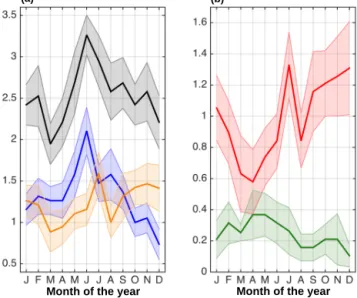
While the two eddy detection methods differ mostly in the number of identified eddies close to the coast, the season of peak eddy generation is very stable for both methods. A pro- nounced seasonality with a maximum of newly formed ed- dies during boreal summer (June/July) is obtained from both methods (Fig. 9). During April to June newly generated ed- dies are mostly cyclonic, while during October to Decem- ber newly generated eddies are mostly anticyclonic (anticy- clones plus ACMEs). These seasonal differences indicate dif- ferent eddy generation mechanisms at play in the TANWA during the different seasons. Different mechanisms for the generation of eddies in eastern boundary upwelling regions have been proposed (e.g., Liang et al., 2012). Barotropic and baroclinic instabilities of the near-coastal currents (Pantoja et

al., 2012) triggered by, e.g., the passage of poleward propa- gating coastal trapped waves (Zamudio et al., 2001, 2007), wind perturbations (Pares-Sierra et al., 1993), or interac- tions of the large-scale circulation with the bottom topog- raphy (Kurian et al., 2011) are the main processes identi- fied for the eddy generation in eastern boundary upwelling regions. In the TANWA, the period of maximum eddy gen- eration (June/July) is characterized by a strong near-surface boundary current, the MC (Lázaro et al., 2005) suggesting dynamic instabilities of the boundary current as an impor- tant generation mechanism. However, there is a difference in peak generation of cyclones and anticyclones. While the maximum generation of cyclones occurs in June during the acceleration phase of the MC, the seasonality of anticyclone generation is not as distinct with weaker maxima in July and at the end of the year. The generation of ACMEs has the main

(a) (b)

Month of the year Month of the year

Number of eddies

Figure 9. Seasonal cycle of the number of eddies generated in the costal region per year based on the results of the OW method as shown in Figs. 7 and 8. In (a) the seasonal cycle of all eddies is marked by the black line, of cyclones by the blue line and of all anticyclonic eddies by the orange line. In (b) the seasonal cycle of anticyclonic eddies is separated into anticyclones (red line) and ACMEs (green line). The shaded areas around the lines represent the standard error.

peak in April to May, which is at the end of the upwelling season. During that period the PUC is likely getting unstable and vanishes later on (Barton, 1989).

The seasonal peak in eddy occurrence appears to propa- gate westwards into the open ocean. To illustrate this, an- nual harmonics are fitted to the number of eddies detected per month in 2^◦×2^◦boxes (Fig. 10). Note, that the phase of a box is only shown when the amplitude is larger than 2.5 eddies per box. After the main generation of cyclones in the coastal area in June, the eddies enter the open ocean in late boreal autumn, passing the Cabo Verde islands and the ventilated gyre regime north of the CVFZ in boreal win- ter/spring. As mentioned before anticyclones are generated 1 to a few months later at the coast (July and October, Novem- ber). They dominantly reach the open ocean in boreal winter and spring and accordingly pass the Cabo Verde islands and the ventilated gyre regime north of the CVFZ in late boreal spring and summer. Note, that the relatively clear signal of the annual harmonic of eddy detections (Fig. 10) also sug- gests that eddies with lifetime > 9 months are more frequent in the TANWA than indicated by the statistical output of the algorithms.

3.4 Mean eddy structure

3.4.1 Surface anomalies related to eddies

For the three types of eddies, composite were constructed from daily SLA, SST, and SSS anomaly fields. An area of 300 km×300 km around every identified eddy center (cen- ter is the maximum value of SLA) was considered (Fig. 11).

Overall we had about 40 000 snapshots of eddies between 1993 and 2013 available to calculate the mean SLA and SST anomalies. To derive mean SSS anomalies, only about 10 000 snapshots were merged because of the shorter time period of the SSS satellite data record (2010–2013).

For anticyclones, we found a positive SLA (maximum value in the eddy core is 6.9 cm (3.02; 11.01 cm), given here as mean and the upper and lower limits of the 68 % quartile range), a positive SST anomaly (maximum value in the eddy core 0.13^◦C (0.03; 0.24^◦C)) and a positive SSS anomaly (maximum value in the eddy core is 0.20 (−0.04;

0.52)). For cyclones, we found a negative SLA (minimum value in core−5.5 cm (−1.57;−7.37 cm)), a negative SST anomaly (minimum value in the core is −0.15^◦C (−0.04;

−0.30^◦C)), and a negative SSS anomaly (minimum value in the core is−0.16 (0.08;−0.48)). However, for the ACMEs (about 20 % of the anticyclones) we found a negative SST anomaly (minimum value in the core is −0.15^◦C (−0.04;

−0.31^◦C)) was observed. The vertical structure of these an- ticyclones as obtained from temperature and salinity profiles revealed the characteristic pattern of ACMEs with a very shallow mode in the upper 100 m or so. ACMEs also have a negative SSS anomaly (minimum value in the core is−0.13 (0.10;−0.33)). For all eddy types, SST dominates sea sur- face density.

Compared to SLA and SST measurements, the satellite- based observations of SSS are afflicted with high uncertain- ties and large measuring gaps. However, in the composite it is possible to detect eddy-type dependent anomalies, even if they are not as clear and circular as the SLA and SST anomalies. The zonally stretched structures in the compos- ites of SSS anomalies may also result from the coarser tem- poral resolution of SSS data (i.e., 10 days) resulting in a smearing of the eddy signal in the direction of propagation.

Note, that the composites of SSS anomalies showed only co- herent eddy structures when selecting energetic eddies (i.e., with a radius between 45 and 70 km and an absolute SLA anomaly > 2 cm). The composites of SLA and SST anoma- lies are much less affected by the restriction with regard to the eddy amplitude.

In summary, the absolute SST and SSS anomalies of all three eddy types are of similar magnitude. The magnitude of absolute SLA of anticyclones and cyclones is also some- how similar, while ACMEs have a weaker SLA signature (which makes them more difficult to be detected and tracked by satellite altimetry). The maximum surface circumpolar velocity is 0.18±0.12 in cyclones, 0.17±0.12 in anticy-