www.biogeosciences.net/13/5865/2016/
doi:10.5194/bg-13-5865-2016
© Author(s) 2016. CC Attribution 3.0 License.
Characterization of “dead-zone” eddies in the eastern tropical North Atlantic
Florian Schütte1, Johannes Karstensen1, Gerd Krahmann1, Helena Hauss1, Björn Fiedler1, Peter Brandt1,2, Martin Visbeck1,2, and Arne Körtzinger1,2
1GEOMAR Helmholtz Centre for Ocean Research Kiel, Kiel, Germany
2Christian-Albrechts-Universität zu Kiel, Kiel, Germany Correspondence to:Florian Schütte (fschuette@geomar.de)
Received: 10 February 2016 – Published in Biogeosciences Discuss.: 22 February 2016 Revised: 10 September 2016 – Accepted: 30 September 2016 – Published: 28 October 2016
Abstract. Localized open-ocean low-oxygen “dead zones”
in the eastern tropical North Atlantic are recently discovered ocean features that can develop in dynamically isolated water masses within cyclonic eddies (CE) and anticyclonic mode- water eddies (ACME). Analysis of a comprehensive oxygen dataset obtained from gliders, moorings, research vessels and Argo floats reveals that “dead-zone” eddies are found in sur- prisingly high numbers and in a large area from about 4 to 22◦N, from the shelf at the eastern boundary to 38◦W. In to- tal, 173 profiles with oxygen concentrations below the min- imum background concentration of 40 µmol kg−1 could be associated with 27 independent eddies (10 CEs; 17 ACMEs) over a period of 10 years. Lowest oxygen concentrations in CEs are less than 10 µmol kg−1while in ACMEs even sub- oxic (< 1 µmol kg−1)levels are observed. The oxygen min- imum in the eddies is located at shallow depth from 50 to 150 m with a mean depth of 80 m. Compared to the surround- ing waters, the mean oxygen anomaly in the core depth range (50 and 150 m) for CEs (ACMEs) is−38 (−79) µmol kg−1. North of 12◦N, the oxygen-depleted eddies carry anoma- lously low-salinity water of South Atlantic origin from the eastern boundary upwelling region into the open ocean. Here water mass properties and satellite eddy tracking both point to an eddy generation near the eastern boundary. In contrast, the oxygen-depleted eddies south of 12◦N carry weak hydro- graphic anomalies in their cores and seem to be generated in the open ocean away from the boundary. In both regions a decrease in oxygen from east to west is identified support- ing the en-route creation of the low-oxygen core through a combination of high productivity in the eddy surface waters and an isolation of the eddy cores with respect to lateral oxy-
gen supply. Indeed, eddies of both types feature a cold sea surface temperature anomaly and enhanced chlorophyll con- centrations in their center. The low-oxygen core depth in the eddies aligns with the depth of the shallow oxygen minimum zone of the eastern tropical North Atlantic. Averaged over the whole area an oxygen reduction of 7 µmol kg−1 in the depth range of 50 to 150 m (peak reduction is 16 µmol kg−1 at 100 m depth) can be associated with the dispersion of the eddies. Thus the locally increased oxygen consumption within the eddy cores enhances the total oxygen consump- tion in the open eastern tropical North Atlantic Ocean and seems to be an contributor to the formation of the shallow oxygen minimum zone.
1 Introduction
The eastern tropical North Atlantic (ETNA: 4 to 22◦N and from the shelf at the eastern boundary to 38◦W; Fig. 1) off northwestern Africa is one of the biologically most produc- tive areas of the global ocean (Chavez and Messié, 2009;
Lachkar and Gruber, 2012). In particular, the eastern bound- ary current system close to the northwestern African coast is a region where northeasterly trade winds force coastal up- welling of cold, nutrient-rich waters, resulting in high pro- ductivity (Bakun, 1990; Lachkar and Gruber, 2012; Messié et al., 2009; Pauly and Christensen, 1995). The ETNA is characterized by a weak large-scale circulation and instead dominated by mesoscale variability (here referred to as ed- dies; Brandt et al., 2015; Mittelstaedt, 1991). Traditionally the ETNA is considered to be “hypoxic”, with minimal oxy-
50 200 0 200 400 600 800 1000
130
120 110
100
90 80
70 60 160
150
140 130 120
35oW 30oW 25oW 20oW 15oW 4oN
8oN 12oN 16oN 20oN
0 2 4 6 8 10
a) b)
% Oxygen (µmol kg-1)
Depth (m) deep OMZ shallow OMZ
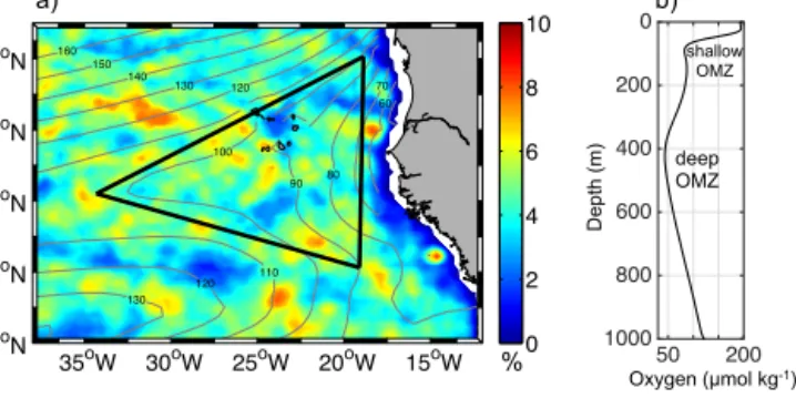
Figure 1. (a)Map of the ETNA including contour lines of the oxy- gen minimum of the upper 200 m (in µmol kg−1)as obtained from the MIMOC climatology (Schmidtko et al., 2013). The color indi- cates the percentage of “dead-zone” eddy coverage per year. The black triangle defines the SOMZ.(b)Mean vertical oxygen profile of all profiles within the SOMZ showing the shallow oxygen min- imum centered around 80 m depth and the deep oxygen minimum centered at 450 m depth.
gen concentrations of marginally below 40 µmol kg−1 (e.g., Stramma et al., 2009; Fig. 1a). The large-scale ventilation and oxygen consumption processes of thermocline waters in the ETNA result in two separate oxygen minima (Fig. 1b): a shallow one with a core depth of about 80 m and a deep one at a core depth of about 450 m (Brandt et al., 2015; Karstensen et al., 2008). The deep minimum is the core of the so-called oxygen minimum zone (OMZ) and is primarily created by sluggish ventilation of the respective isopycnals (Luyten et al., 1983; Wyrtki, 1962). It extends from the eastern bound- ary into the open ocean and is located in the so-called shadow zone of the ventilated thermocline, with the more energetic circulation of the subtropical gyre in the north and the equa- torial region in the south (Karstensen et al., 2008; Luyten et al., 1983). The shallow oxygen minimum intensifies from the Equator towards the north with minimal values near the coast at about 20◦N (Brandt et al., 2015; Fig. 1a). It is assumed that the shallow oxygen minimum originates from enhanced biological productivity and an increased respiration associ- ated with sinking particles in the water column (Brandt et al., 2015; Karstensen et al., 2008; Wyrtki, 1962).
The eddies act as a major transport agent between coastal waters and the open ocean (Schütte et al., 2016a), which is a well-known process for all upwelling areas in the world oceans (Capet et al., 2008; Chaigneau et al., 2009; Correa- Ramirez et al., 2007; Marchesiello et al., 2003; Nagai et al., 2015; Schütte et al., 2016a; Thomsen et al., 2015). In the ETNA, most eddies are generated near the eastern bound- ary; Rossby wave dynamics and the basin-scale circulation force these eddies to propagate westwards (Schütte et al., 2016a). Open-ocean eddies with particularly high South At- lantic Central Water (SACW) fractions in their cores have been found far offshore in regions dominated by the much saltier North Atlantic Central Water (NACW; Karstensen et
al., 2015; Pastor et al., 2008). Weak lateral exchange across the eddy boundaries is most likely the reason for the isolation (Schütte et al., 2016a). The impact of eddy transport on the coastal productivity (equivalent to other upwelling-related properties) was investigated by Gruber et al. (2011), who were able to show that high (low) eddy-driven transports of nutrient-rich water from the shelf into the open-ocean results in lower (higher) biological production on the shelf. Besides acting as export agents for coastal waters and conservative tracers, coherent eddies have been reported to establish and maintain an isolated ecosystem changing non-conservative tracers with time (Altabet et al., 2012; Fiedler et al., 2016;
Hauss et al., 2016; Karstensen et al., 2015; Löscher et al., 2015). Coherent/isolated mesoscale eddies can exist over pe- riods of several months or even years (Chelton et al., 2011).
During that time the biogeochemical conditions within these eddies can evolve very different from the surrounding water masses (Fiedler et al., 2016). Hypoxic to suboxic oxygen lev- els have been observed in cyclonic eddies (CEs) and anticy- clonic mode-water eddies (ACMEs) at shallow depth and just beneath the mixed layer (ML, about 50 to 100 m; Karstensen et al., 2015). The creation of the low-oxygen cores in the ed- dies have been attributed to the combination of several fac- tors (Karstensen et al., 2015): high productivity in the surface waters of the eddy (Hauss et al., 2016; Löscher et al., 2015), enhanced respiration of sinking organic material at subsur- face depth (Fiedler et al., 2016; Fischer et al., 2016) and an
“isolation” of the eddy core from exchange with surrounding and better-oxygenated water (Karstensen et al., 2016). The intermittent nature of the oxygen depletion and the combi- nation of high respiration with sluggish oxygen transport re- sembles what is known as “dead zone” in other aquatic sys- tem (lakes, shallow bays), and therefore the term “dead-zone eddies” has been introduced (Karstensen et al., 2015). So far the profound impacts on behavior of microbial (Löscher et al., 2015) and metazoan (Hauss et al., 2016) communities has been documented inside the eddies. For example, the appear- ance of denitrifying bacteria, typically absent from the open tropical Atlantic, has been observed (Löscher et al., 2015) via the detection of nirS gene transcripts (the key functional marker for denitrification). However, the close-to-Redfield N : P stoichiometry in ACMEs in the ETNA (Fiedler et al., 2016) does not suggest a large-scale net loss of bioavail- able nitrogen via denitrification. The key point in changing non-conservative tracers in the eddy cores is the physical- biological coupling, which is strongly linked to the verti- cal velocities of submesoscale physics, stimulating primary production (upward nutrient flux) in particular under olig- otrophic conditions (Falkowski et al., 1991; Levy et al., 2001;
McGillicuddy et al., 2007). The detailed understanding of the physical and biogeochemical processes and their linkage in eddies is still limited (Lévy et al., 2012). Consequently the relative magnitude of eddy-dependent vertical nutrient flux, primary productivity and associated enhanced oxygen consumption or nitrogen fixation/denitrification in the eddy
cores and accordingly the contribution to the large-scale oxy- gen or nutrient distribution is fairly unknown.
In order to further investigate the physical, biogeochemical and ecological structure of “dead-zone” eddies, an interdis- ciplinary field study was carried out in winter 2013/spring 2014 in the ETNA, north of Cape Verde, using dedicated ship, mooring and glider surveys supported by satellite and Argo float data. The analysis of the field study data revealed surprising results regarding eddy metagenomics (Löscher et al., 2015), zooplankton communities (Hauss et al., 2016), carbon chemistry (Fiedler et al., 2016) and nitrogen cycling (Karstensen et al., 2016). Furthermore, analyses of particle flux time series, using sediment trap data from the Cape Verde Ocean Observatory (CVOO), were able to confirm the impact of highly productive “dead-zone” eddies on deep lo- cal export fluxes (Fischer et al., 2016). In this paper we inves- tigate “dead-zone” eddies detected from sea level anomaly (SLA) and sea surface temperature (SST) data based on methods described by Schütte et al. (2016a). We draw a con- nection between the enhanced consumption and associated low-oxygen concentration in eddy cores and the formation of the regional observed shallow oxygen minimum. To as- sess the influence of oxygen-depleted eddies on the oxygen budget of the upper water column, a sub-region between the ventilation pathways of the subtropical gyre and the zonal current bands of the equatorial Atlantic was chosen and in- vestigated in more detail. This region includes the most pro- nounced shallow oxygen minimum zone (SOMZ; Fig. 1a).
The probability of “dead-zone” eddy occurrence per year is more or less evenly distributed in the ETNA (Fig. 1a). Par- ticularly in the SOMZ there seems to be neither a distinctly high nor an explicitly low “dead-zone” eddy occurrence. Due to the absence of other ventilation pathways in this zone, the influence of “dead-zone” eddies on the shallow oxygen minimum budget may be important and a closer examina- tion worth the effort. We determine the average characteris- tics of “dead-zone” eddies in the ETNA, addressing their hy- drographic features as well as occurrence, distribution, gen- eration and frequency. Based on oxygen anomalies and eddy coverage we estimate their contribution to the oxygen budget of the SOMZ. The paper is organized as follows. Section 2 addresses the different in situ measurements, satellite prod- ucts and methods we use. Our results are presented in Sect. 3, discussed in Sect. 4 and summarized in Sect. 5.
2 Data and methods 2.1 In situ data acquisition
For our study we employ a quality-controlled database com- bining shipboard measurements, mooring data and Argo float profiles as well as autonomous glider data taken in the ETNA. For details on the structure and processing of the database see Schütte et al. (2016a). For this study we ex-
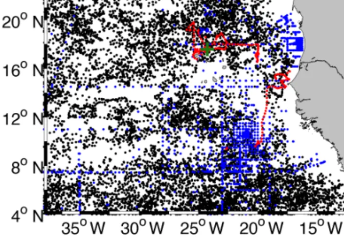
Figure 2.Map of the ETNA containing all available profiles be- tween 1998 and 2014. The green cross marks the CVOO position, blue dots mark shipboard conductivity–temperature–depth (CTD) stations, red dots mark the locations of glider profiles and black dots locations of Argo float profiles.
tended the database in several ways. The region was ex- panded to now cover the region from 0 to 22◦N and 13 to 38◦W (see Fig. 2). We then included data from five recent ship expeditions (RVIslandiaISL_00314, RVMeteorM105, M107, M116, M119), which sampled extensively within the survey region. Data from the two most recent deployment pe- riods of the CVOO mooring from October 2012 to Septem- ber 2015 as well as Argo float data for the years 2014 and 2015 were also included. Furthermore, oxygen measure- ments of all data sources were collected and integrated into the database. As the last modification of the database we included data from four autonomous gliders that were de- ployed in the region and sampled two ACMEs and one CE.
Glider IFM11 (deployment ID: ifm11_depl01) was deployed on 13 March 2010. It covered the edge of an ACME on 20 March and recorded data in the upper 500 m. Glider IFM05 (deployment ID: ifm05_depl08) was deployed on 13 June 2013. It crossed a CE on July 26 and recorded data down to 1000 m depth. IFM12 (deployment ID: ifm12_depl02) was deployed on 10 January 2014 north of the Cape Verde island São Vicente and surveyed temperature, salinity and oxygen to 500 m depth. IFM13 (deployment ID: ifm13_depl01) was deployed on 18 March 2014 surveying temperature, salinity and oxygen to 700 m depth. IFM12 and IFM13 were able to sample three complete sections through an ACME. All glider data were internally recorded as a time series along the flight path, while for the analysis the data was interpolated onto a regular pressure grid of 1 dbar resolution (see also Thom- sen et al., 2015). Gliders collect a large number of relatively closely spaced slanted profiles. To reduce the number of de- pendent measurements, we limited the number of glider pro- files to one every 12 h. All four autonomous gliders were equipped with Aanderaa optodes (3830) installed in the aft
section of the devices. A recalibration of the optode calibra- tion coefficients was determined on dedicated conductivity–
temperature–depth (CTD) casts following the procedures of (Hahn et al., 2014). These procedures also estimate and cor- rect the delays caused by the slow optode response time (more detailed information can be found in Hahn et al., 2014, and Thomsen et al., 2015). As gliders move through the water column the oxygen measurements are not as stable as those from moored optodes analyzed by Hahn et al. (2014). We thus estimate their measurement error to about 3 µmol kg−1. The processing and quality control procedures for tempera- ture and salinity data from shipboard measurements, moor- ing data and Argo floats has already been described by Schütte et al. (2016a). The processing of the gliders’ tem- perature and salinity measurements is described in Thomsen et al. (2015). Oxygen measurements of the shipboard surveys were collected with Seabird SBE 43 dissolved oxygen sen- sors attached to Seabird SBE 9plus or SBE 19 CTD systems.
Sampling and calibration followed the procedures detailed in the GO-SHIP manuals (Hood et al., 2010). The resulting measurement error were≤1.5 µmol kg−1. Within the CVOO moorings, a number of dissolved oxygen sensors (Aanderaa optodes type 3830) were used.
Calibration coefficients for moored optodes were deter- mined on dedicated CTD casts and additional calibrated in the laboratory with water featuring 0 % air saturation before deployment and after recovery following the procedures de- scribed by Hahn et al. (2014). We estimate their measurement error at < 3 µmol kg−1. For the few Argo floats equipped with oxygen sensors a full calibration is usually not available and only a visual inspection of the profiles was done before in- cluding the data into the database. The different manufactur- ers of Argo float oxygen sensors specify their measurement error at least better than 8 µmol kg−1 or 5 %, whichever is larger. Note that early optodes can be significantly outside of this accuracy range, showing offsets of 15–20 µmol kg−1, in some cases even higher.
As a final result the assembled in situ database of the ETNA contains 15 059 independent profiles (Fig. 2). All profiles include temperature, salinity and pressure measure- ments while 38.5 % of all profiles include oxygen measure- ments. The database is composed of 13 % shipboard, 22.5 % CVOO mooring, 63 % Argo float and 1.5 % glider profiles.
To determine the characteristics of different eddy types from the assembled profiles, we separated them into CEs, ACMEs and the “surrounding area” not associated with eddy-like structures following the approach of Schütte et al. (2016a).
2.2 Satellite data
We detected and tracked eddies following the procedures de- scribed in Schütte et al. (2016a). In brief we used 19 years of the delayed-time “all-sat-merged” reference dataset of SLA (version 2014). The data are produced by Ssalto/Duacs and distributed by AVISO (Archiving, Validation, and In-
terpretation of Satellite Oceanographic), with support from CNES (http://www.aviso.altimetry.fr/duac/). We used the multi-mission product, which is mapped on a 1/4◦×1/4◦ Cartesian grid and has a temporal resolution of 1 day. The anomalies were computed with respect to a 19-year mean.
The SLA and geostrophic velocity anomalies also provided by AVISO were chosen for the time period January 1998 to December 2014.
For SST the dataset “Microwave Infrared Fusion Sea Sur- face Temperature” from Remote Sensing Systems (www.
remss.com) is used. It is a combination of all operational microwave (MW) radiometer SST measurements (TMI, AMSR-E, AMSR2, WindSat) and infrared (IR) SST mea- surements (Terra MODIS, Aqua MODIS). The dataset thus combines the advantages of the MW data (through-cloud capabilities) with the IR data (high spatial resolution). The SST values are corrected using a diurnal model to create a foundation SST that represents a 12:00 LT temperature (www.remss.com). Daily data with 9 km resolution from Jan- uary 2002 to December 2014 are considered.
For sea surface chlorophyll (Chl) data we use the MODIS/Aqua Level 3 product available at http://oceancolor.
gsfc.nasa.gov provided by the NASA. The data were mea- sured via IR and are therefore cloud cover dependent. Daily data mapped on a 4 km grid from January 2006 to December 2014 are selected.
2.3 Low-oxygen eddy detection and surface composites In order to verify whether low-oxygen concentrations (< 40 µmol kg−1)at shallow depth (above 200 m) are asso- ciated with eddies we applied a two step procedure. First, all available oxygen measurements of the combined in situ datasets are used to identify negative oxygen anomalies with respect to the climatology. Next, the satellite-data- based eddy detection results (Schütte et al., 2016a) were matched in space and time with the location of anomalously low-oxygen profiles. In this survey the locations of 173 of 180 low-oxygen profiles coincide with surface signatures of mesoscale eddies. Schütte et al. (2016a) showed that ACMEs can be distinguished in the ETNA from “normal” anticy- clonic eddies by considering the SST anomaly (cold in case of ACMEs) and sea surface salinity (SSS) anomaly (fresh in case of ACMEs) in parallel to the respective SLA anomaly.
The satellite-based estimates of SLA and SST used in this study are obtained by subtracting low-pass filtered (cutoff wavelength of 15◦longitude and 5◦latitude) values from the original data to exclude large-scale variations and preserve only the mesoscale variability (see Schütte et al., 2016a for more detail). All eddy-like structures with low-oxygen pro- files are visually tracked in the filtered SLA (sometimes SST data) backward and forward in time in order to obtain eddy propagation trajectories. The surface composites of satellite- derived SLA, SST and Chl data consist of 150 km×150 km
−50 0 50 100 0
50 100 150 200 250 300 350 400 450 500
Depth (m)
Oxygen difference (µmol kg−1)
Sigma-theta (kg m-3)
Oxygen (µmol kg-1)
0 50 100 150
Depth (m)
0 50 100 150 200 250 300 350 400 450
500
Salinity
Oxygen (µmol kg-1)
(a) (b) (c)
Depth (m) Depth (m)
Oxygen (µmol kg-1) Oxygen difference (µmol kg-1)
Figure 3. (a)Salinity–σθ diagram with color indicating the oxygen concentrations. The black line separates the 173 profiles with minimum oxygen concentration of < 40 µmol kg−1(left side/more SACW characteristics) from profiles of the surrounding water (right side/more NACW characteristics), taken from the same devices shortly before and after the encounter with a low-oxygen eddy. (b)Mean oxygen concentration vs. depth of the coastal region (east of 18◦W, solid black line), of all CEs (solid blue line) and all ACMEs (solid green line) with available oxygen measurements. The dashed line represents the reconstructed mean oxygen concentration for the same CEs (blue) and ACMEs (green).(c)Difference between the reconstructed and measured oxygen concentrations in CEs (blue) and ACMEs (green) with associated standard deviation (shaded area).
snapshots around the obtained eddy centers. For construction of the composites the filtered SLA and SST are used as well.
2.4 Reconstruction of oxygen concentrations in low-oxygen eddy cores
About 30 % of the profiles from the combined in situ dataset conducted in CEs or ACMEs do not have oxygen measure- ments available. However, we are only interested in oxygen measurements in isolated CE or ACME cores. These isolated eddy cores carry anomalously low-salinity SACW of coastal origin, while the surrounding waters are characterized by an admixture of more saline NACW (Schütte et al., 2016a). All eddies that show a low-salinity and cold core indicate that (i) they have been generated near the coast and (ii) their core has been efficiently isolated from surrounding waters. The salinity–σθdiagram (Fig. 3a) of open-ocean (west of 19◦W) profiles shows a correlation between low-salinity eddy cores and low-oxygen concentrations. Moreover, it indicated that the oxygen content in the isolated eddies is decreasing from east to west. In order to compensate for missing oxygen measurements on many of the profiles we derive a salinity–
oxygen relation but also consider the “age” of the eddy (time since the eddy left the eastern boundary) and an oxygen con- sumption rate within the eddy core. The oxygen consumption rate is estimated from the difference between the observed oxygen and a reference profile (the mean of all profiles east of 18◦W in the eastern boundary region; Fig. 3a), the dis- tance from the eastern boundary, and the propagation speed (3 km d−1; see Schütte et al., 2016a). The mean eddy con- sumption rate is now the difference from the initial oxygen
condition and the observed oxygen concentration in the eddy core divided by the eddy age (distance divided by propaga- tion speed). For eddy profiles without oxygen measurements but SACW water mass characteristics (less saline and colder water than surrounding water) we can assume a strong iso- lation of the eddy and thus a lowering in oxygen. Using the coastal reference profile (Fig. 3), oxygen consumption rate and the distance from the coast an oxygen profile is recon- structed for all isolated CEs and ACMEs. To validate the method we reconstructed the oxygen profiles for the eddies with available oxygen measurements and compared them (Fig. 3b). On average an uncertainty of±12 (16) µmol kg−1 is associated with the reconstructed oxygen values (Fig. 3c) of CEs (ACMEs). Depending on the intensity of isolation of the eddy core, lateral mixing could have taken place, which is assumed to be zero in our method. However, this approach enables us to enlarge the oxygen dataset by 30 %. We consid- ered the reconstructed oxygen profiles only to estimate the mean structure of oxygen anomaly.
2.5 Mean vertical oxygen anomaly of low-oxygen eddies and their impact on the SOMZ
To illustrate mean oxygen anomalies for CEs and ACMEs as a function of depth and radial distance, all oxygen profiles (observed and reconstructed) were sorted with respect to a normalized distance, which is defined as the actual distance of the profile from the eddy center divided by the radius of the eddy (the shape and thus the radius of the eddy are gained from the streamline with the strongest swirl velocity around a center of minimum geostrophic surface velocity). The oxy-
35oW 30oW 25oW 20oW 15oW 4oN
8oN 12oN 16oN 20oN 150
130
110
80 60
100
120
0 5 10 15 20 25 30 35 40
Oxygen (µmol kg-1)
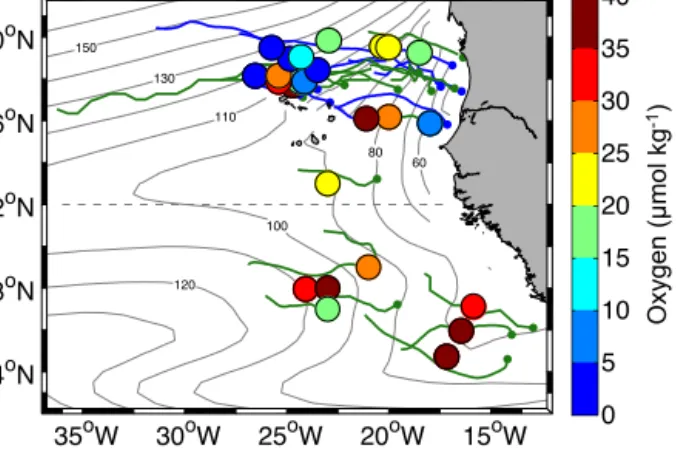
Figure 4. Minimum oxygen concentration (contour lines, µmol kg−1)in the ETNA between the surface and 200 m depth as obtained from the MIMOC climatology (Schmidtko et al., 2013).
Superimposed colored dots are all low-oxygen measurements (be- low 40 µmol kg−1in the upper 200 m) which could be associated with eddy-like structures. The size of the dots represents a typical size of the mesoscale eddies. The associated trajectories of the ed- dies are shown in green for ACMEs and in blue for cyclones. The oxygen concentrations are from the combined dataset of shipboard, mooring, glider and Argo float measurements.
gen profiles were grouped and averaged onto a grid of 0.1 in- crements between 0 and 1 of the normalized radial distance.
Finally a running mean over three consecutive horizontal grid points was applied. A mean oxygen anomaly for the CEs and the ACMEs was constructed by the comparison with the oxy- gen concentrations in the surrounding waters. To illustrate the influence of the reconstructed oxygen values, the mean oxygen anomaly is also constructed based only on original measured oxygen values, and both anomalies are shown for comparison.
An oxygen deficit profile due to “dead-zone” eddies in the SOMZ is derived by building an oxygen anomaly on density surfaces (O20)separating CEs and ACMEs. The de- rived anomalies are multiplied by the mean number of ed- dies dissipating in the SOMZ per year (n) and weighted by the area of the eddy compared to the total area of the SOMZ (ASOMZ=triangle in Fig. 1a). Differences in the mean isopycnal layer thickness of each eddy type and the SOMZ are considered by multiplying the result with the ra- tio of the mean Brunt–Väisälä frequency (N2)outside and in- side the eddy, resulting in an apparent oxygen utilization rate (µmol kg−1yr−1)due to “dead-zone” eddies in the SOMZ on density layers:
aOUR=nO20π rEddy2 N2SOMZ ASOMZN2Eddy,
whererEddyis the mean radius of the eddies.
3 Results
3.1 Low-oxygen eddy observation from in situ data Several oxygen measurements in the ETNA with anoma- lously low-oxygen concentrations, which is defined here as an oxygen concentration below 40 µmol kg−1 (Stramma et al., 2009) could be identified from Argo floats, ship surveys, glider missions and from the CVOO mooring (Fig. 4). In total, 27 independent eddies with oxygen values
< 40 µmol kg−1 in the upper 200 m were sampled with 173 profiles from 25 different platforms (Table 1). Almost all of the observed anomalous low-oxygen values could be asso- ciated with mesoscale structures at the sea surface (CEs or ACMEs) from satellite data.
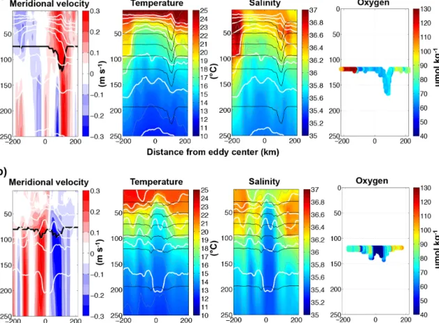
In situ measurements for meridional velocity, tempera- ture, salinity and oxygen of the CVOO mooring during the westward passage of one CE and one ACME with low- oxygen concentrations are chosen to introduce the two dif- ferent eddy types and their vertical structure based on tem- porally high-resolution data (Fig. 5). From October 2006 to December 2006 (Fig. 5a), a CE passed the CVOO mooring position on a westward trajectory. At its closest, the eddy center was located about 20 km north of the mooring. The meridional velocities show a strong cyclonic rotation (first southward, later northward) with velocity maxima between the surface and 50 m depth at the edges of the eddy. In the core of the CE, the water mass was colder and less saline than the surrounding water, the ML depth is reduced and the isopycnals are shifted upwards. The oxygen content of the eddy core was reduced by about 60 µmol kg−1at 115 m depth (or at the isopycnal surface 26.61 kg m−3)compared to surrounding waters, which have a mean (±1 standard de- viation) oxygen content of 113 (±38) µmol kg−1at around 150 m depth or 26.60 (±0.32) kg m−3during the mooring pe- riod between 2006 and 2014. Schütte et al. (2016a) showed that around 52 % of the eddies in the ETNA represents CEs.
They have a marginally smaller radius, rotate faster and have a shorter lifetime compared to the anticyclonic eddies, which is also shown in other observational studies of Chaigneau et al. (2009), Chelton et al. (2011), and theoretically suggested by Cushman-Roisin et al. (1990).
From January 2007 to March 2007 (Fig. 5b), an ACME passed the CVOO mooring position. The core of the west- ward propagating eddy passed about 13 km north of the mooring. The velocity field shows strong subsurface anti- cyclonic rotation at the depth of the core, i.e., between 80 and 100 m. In contrast to “normal” anticyclonic eddies, the water mass in the core of an ACME is colder and less saline than the surrounding waters. The isopycnals above the core are elevated resulting in shallower MLs both re- sembling a cyclone. Beneath the core, the isopycnals are strongly depressed as in a normal anticyclone. Thus, dynam- ically this resembles a mode-water anticyclone, an eddy type which is well known from local single observations in al-
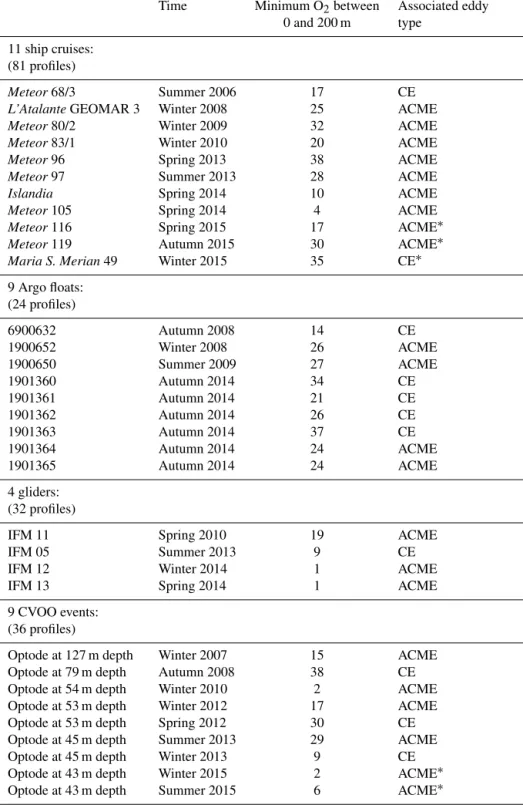
Table 1.Available oxygen measurements below 40 µmol kg−1in the ETNA. The∗indicates recent observations which are not included in Fig. 4 due to not existent delayed time satellite products.
Time Minimum O2between Associated eddy 0 and 200 m type
11 ship cruises:
(81 profiles)
Meteor68/3 Summer 2006 17 CE
L’AtalanteGEOMAR 3 Winter 2008 25 ACME
Meteor80/2 Winter 2009 32 ACME
Meteor83/1 Winter 2010 20 ACME
Meteor96 Spring 2013 38 ACME
Meteor97 Summer 2013 28 ACME
Islandia Spring 2014 10 ACME
Meteor105 Spring 2014 4 ACME
Meteor116 Spring 2015 17 ACME∗
Meteor119 Autumn 2015 30 ACME∗
Maria S. Merian49 Winter 2015 35 CE∗
9 Argo floats:
(24 profiles)
6900632 Autumn 2008 14 CE
1900652 Winter 2008 26 ACME
1900650 Summer 2009 27 ACME
1901360 Autumn 2014 34 CE
1901361 Autumn 2014 21 CE
1901362 Autumn 2014 26 CE
1901363 Autumn 2014 37 CE
1901364 Autumn 2014 24 ACME
1901365 Autumn 2014 24 ACME
4 gliders:
(32 profiles)
IFM 11 Spring 2010 19 ACME
IFM 05 Summer 2013 9 CE
IFM 12 Winter 2014 1 ACME
IFM 13 Spring 2014 1 ACME
9 CVOO events:
(36 profiles)
Optode at 127 m depth Winter 2007 15 ACME
Optode at 79 m depth Autumn 2008 38 CE
Optode at 54 m depth Winter 2010 2 ACME
Optode at 53 m depth Winter 2012 17 ACME
Optode at 53 m depth Spring 2012 30 CE
Optode at 45 m depth Summer 2013 29 ACME
Optode at 45 m depth Winter 2013 9 CE
Optode at 43 m depth Winter 2015 2 ACME∗
Optode at 43 m depth Summer 2015 6 ACME∗
P173 profiles P
27 different eddies
most all ocean basins (globally: Kostianoy and Belkin, 1989;
McWilliams, 1985 (“submesoscale coherent vortices”); in the North Atlantic: Riser et al., 1986; Zenk et al., 1991 and Bower et al., 1995; Richardson et al., 1989; Armi and Zenk,
1984 (“Meddies”); in the Mediterranean Sea: Tauper-Letage et al., 2003 (“Leddies”); in the North Sea: Van Aken et al., 1987; in the Baltic Sea: Zhurbas et al., 2004; in the Indian Ocean: Shapiro and Meschanov, 1991 (“Reddies”); in the
Figure 5.Meridional velocity, temperature, salinity and oxygen of an exemplary(a)CE and(b)ACME at the CVOO mooring. Both eddies passed the CVOO on a westward trajectory with the eddy center north of the mooring position (CE 20 km, ACME 13 km). The CE passed the CVOO from October to December 2006 and the ACME between January and March 2007. The thick black lines in the velocity plots indicate the position of an upward looking ADCP. Below that depth calculated geostrophic velocity is shown. The white lines represent density surfaces inside the eddies and the thin grey lines isolines of temperature and salinity, respectively. Thin black lines in the temperature and salinity plot mark the vertical position of the measuring devices. On the right a time series of oxygen is shown from the one sensor available at nominal 120 m depth.
North Pacific: Lukas and Santiago-Mandujano, 2001; Mole- maker et al., 2015 (“Cuddies”); in the South Pacific: Stramma et al., 2013; Colas et al., 2012; Combes et al., 2015; Thomsen et al., 2015 and Nof et al., 2002 (“Teddies”); in the Arctic:
D’Asaro, 1988; Oliver et al., 2008). For the majority of the observed mode-water-type eddies the depressed isopycnals in deeper water mask the elevated isopycnals in the shallow water in terms of geostrophic velocity, resulting in an anti- cyclonic surface rotation and a weak positive SLA (Gaube et al., 2014).
In contrast to most of the ACMEs reported, the CVOO ACME eddy core is located at very shallow depth, just beneath the ML. The oxygen content in the eddy’s core recorded from the CVOO mooring is strongly decreased with values around 19 µmol kg−1 at 123 m depth (or 26.50 kg m−3) compared to the surrounding waters (113 (±38) µmol kg−1). Within the entire time series, the CVOO mooring recorded the passage of several ACMEs with even lower oxygen concentrations (for more information see
Karstensen et al., 2015, or Table 1). Recent model studies suggest that ACMEs represent a non-negligible part of the worlds eddy field, particular in upwelling regions (Combes et al., 2015; Nagai et al., 2015). Schütte et al. (2016a) could show, based on observational data, that ACMEs represent around 9 % of the eddy field in the ETNA. Their radii are in the order of the first baroclinic-mode Rossby radius of de- formation and their eddy cores are well isolated (Schütte et al., 2016a).
3.2 Combining in situ and satellite data for low-oxygen eddy detection in the ETNA
Combining the location and time of in situ detection of low- oxygen eddies with the corresponding SLA satellite data re- veals a clear link to the surface manifestation of mesoscale structures, CEs and ACMEs (Fig. 4). Composite surface sig- natures for SLA, SST and Chl from all anomalous low- oxygen eddies as identified in the in situ dataset are shown
Distance from eddy core [km]
Distance from eddy core [km]
SLA (ACME)
−100 −50 0 50 100
−100
−50
0
50
100 [cm]−5
0 5
Distance from eddy core [km]
Distance from eddy core [km]
SLA (Cyclone)
−100 −50 0 50 100
−100
−50
0
50
100 [cm]−5
0 5
Distance from eddy core [km]
Distance from eddy core [km]
SST (ACME)
−100 −50 0 50 100
−100
−50 0 50 100
[/circ C]
−0.1
−0.05 0 0.05 0.1 0.15
Distance from eddy core [km]
Distance from eddy core [km]
SST (Cyclone)
−100 −50 0 50 100
−100
−50
0
50
100 [/circ C]
−0.1
−0.05 0 0.05 0.1 0.15
Distance from eddy core [km]
Distance from eddy core [km]
Chl (ACME)
−100 −50 0 50 100
−100
−50 0 50 100
[log(mg m−3)]
−1
−0.5 0 0.5 1
Distance from eddy core [km]
Distance from eddy core [km]
Chl (Cyclone)
−100 −50 0 50 100
−100
−50
0
50
100
[log(mg m−3)]
−1
−0.5 0 0.5 1 100
50
0
-50
-100
Distance from eddy center (km)
Distance from eddy center (km)
100
50
0
-50
-100
100 50 0 -50 -100 100 50 0 -50 -100 100 50 0 -50 -100 100 50 0 -50 -100 100 50 0 -50 -100 100 50 0 -50 -100
SLA (Cyclone) SST (Cyclone) Chl (Cyclone)
SLA (ACME) SST (ACME) Chl (ACME)
100
50
0
-50
-100
100
50
0
-50
-100
100
50
0
-50
-100 100
50
0
-50
-100
(a)
(b)
5
2.5
0
-2.5
-5
5
2.5
0
-2.5
-5
0.15
0.75
0
-0.75
-0.15
0.15
0.75
0
-0.75
-0.15
1
0.5
0
-0.5
-1
1
0.5
0
-0.5
-1
(cm) (°C) (log mg m-3)
(cm) (°C) (log mg m-3)
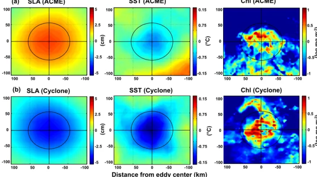
Figure 6.Composites of surface signature for SLA, SST and Chl from all detected low-oxygen eddies:(a)ACMEs and(b)CEs. The solid black cross marks the eddy center and the solid black circle the average radius. Due to significant cloud cover the number of Chl data are much less when compared to the SLA and SST data; thus there is more lateral structure.
−0.2 −0.1 0 0.1 0.2
50 100 150 200 250 300 350 400 450 500
Depth (m)
aOUR (µmol kg−1 day−1)
Figure 7.Depth profiles of a mean apparent oxygen utilization rate (aOUR, µmol kg−1d−1)within CEs (blue) and ACMEs (green) in the ETNA with associated standard deviation (shaded area). De- rived by using the propagation time of each eddy, an initial coastal oxygen profile and the assumption of linear oxygen consumption (based on depth layers).
in Fig. 6. The ACME composites are based on 17 indepen- dent eddies and on 922 surface maps. The detected ACMEs are characterized by an elevation of SLA, which is associated with an anticyclonic rotation at the sea surface. The magni- tude of the SLA displacement is moderate compared to nor- mal anticyclones and CEs (Schütte et al., 2016a). More dis- tinct differences to normal anticyclones are the cold-water anomaly and the elevated Chl concentrations in the eddy center of the ACMEs. Normal anticyclones are associated with elevated SST and reduced Chl concentrations. Through a combination of the different satellite products (SLA, SST, SSS) it is possible to determine low-oxygen eddies from satellite data alone (further details of the ACME tracking and the average satellite surface signatures (SLA, SST, SSS) of all eddy types (CEs, anticyclones and ACMEs) identified in 19 years of satellite data in Schütte et al., 2016a).
The composite mean surface signature for low-oxygen CEs is based on 10 independent eddies and on 755 surface maps. The CEs are characterized by a negative SLA and SST anomaly. The observed negative SST anomaly of the low-oxygen CEs is twice as large (core value CE: −0.12 (±0.2)◦C; core value ACME:−0.06 (±0.2)◦C) as the corre- sponding anomaly of the ACMEs. The Chl concentration in the eddy center is also higher for CEs compared to ACMEs (core value CE: 0.35 (±0.22) log mg m−3; core value ACME:
0.21 (±0.17) log mg m−3). Note that we only considered the measured low-oxygen ACMEs and CEs from Table 1 to de- rive the composites.
ACME
−50 0 50
50 100 150 200 250 300 350 400 450
500 −150
−100
−50 0 50 100 150
Oxygen anomaly (µmol kg-1) ACME
−50 0 50
50 100 150 200 250 300 350 400 450 500 Cyclone
Depth [m]
−50 0 50
50 100 150 200 250 300 350 400 450 500
Distance from eddy center (km)
Depth (m)
−150−100−50 0 50 50
100 150 200 250 300 350 400 450 500
Depth (m)
-100 -50 0
Oxygen anomaly (µmol kg-1)
(a) (b) (c)
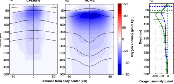
Figure 8.Vertical structure of oxygen from the composite(a)CE and(b)ACME in the ETNA presented as a half section across the eddies.
The left side of both panels (−60 to 0 km) is based on reconstructed and measured oxygen profiles whereas the right side (0 to 60 km) is based on measured oxygen profiles only. Both methods are shown against the normalized radial distance. The blackb lines represents the density surfaces inside the eddies.(c)Mean profiles of the oxygen anomalies based on measured profiles only; green lines are associated with ACMEs and blue to CEs. Horizontal lines indicate the standard deviation of the oxygen anomaly at selected depths. The thick dashed lines indicates the mean ML within the different eddy types. The grey vertical dashed line represents zero oxygen anomaly.
Using the eddy-dependent surface signatures in SLA, SST and Chl the low-oxygen eddies could be tracked and an eddy trajectory could be derived (e.g., Fig. 4). All detected ed- dies were propagating westward into the open ocean. North of 12◦N, most of the eddies set off near the coast, whereas south of 12◦N the eddies seem to be generated in the open ocean. Detected CEs have a tendency to deflect poleward on their way into the open ocean (Chelton et al., 2011), whereas ACMEs seem to have no meridional deflection. However, during their westward propagation the oxygen concentra- tion within the low-oxygen eddy cores decreases with time.
Using the propagation time and an initial coastal oxygen profile (Fig. 3b), a mean apparent oxygen utilization rate per day could be derived for all sampled eddies (Fig. 7).
On average the oxygen concentration decreases by about 0.19±0.08 µmol kg−1d−1in the core of an isolated ACME but has no significant trend in the core of an isolated CE (0.10±0.12 µmol kg−1d−1). This is in the range of recently published aOUR estimates for single observations of CEs (Karstensen et al., 2015) and ACMEs (Fiedler et al., 2016).
3.3 Mean oxygen anomalies from low-oxygen eddies in the ETNA
In Fig. 8 we compare the mean oxygen anomalies based purely on observations with those based on the extended pro- file database, including observed and reconstructed oxygen values (see Sect. 2.4). It shows the mean oxygen anomalies against the surrounding water for CE (Fig. 8a) and ACME (Fig. 8b) vs. depth and normalized radial distance. On the left side of each panel the anomaly is based on the observed
and reconstructed oxygen values (736 oxygen profiles; 575 in CEs; 161 in ACMEs), whereas on the right side the anomaly is based only on the observed oxygen measurements (504 oxygen profiles; 395 in CEs; 109 in ACMEs). The distinct mean negative oxygen anomalies for CEs and ACMEs indi- cate the low-oxygen concentrations in the core of both eddy types compared to the surrounding water. The strongest oxy- gen anomalies are located in the upper water column, just beneath the ML. CEs feature maximum negative anomalies of around−100 µmol kg−1at around 70 m depth in the eddy core, with a slightly more pronounced oxygen anomaly when including the reconstructed values (left side of Fig. 8) com- pared to the oxygen anomaly based purely on observation (right side of Fig. 8a). This is contrary for the ACME with stronger oxygen anomalies on the right part than on the left (Fig. 8b). Both methods deliver maximum negative anoma- lies of around −120 µmol kg−1 at around 100 m depth in the ACME core. At that depth, the diameter of the mean oxygen anomaly is about 100 km for ACMEs and 70 km for CEs (the eddy core is defined here as the area of oxy- gen anomalies smaller than−40 µmol kg−1). Beneath 150 m depth, magnitude and diameter of the oxygen anomalies de- crease rapidly for both eddy types. Figure 8c is based on both the in situ and reconstructed oxygen values and shows the horizontal mean oxygen anomaly profile of each eddy type against depth obtained by horizontally averaging the oxygen anomalies shown in Fig. 8a and b. The maximum anomalies are−100 µmol kg−1 at around 90 m for ACMEs and−55 µmol kg−1at around 70 m for cyclones. Both eddy types have the highest oxygen variance directly beneath the
ML (in the eddy core) or slightly above the eddy core. The oxygen anomaly (and associated variance) decreases rapidly with depth beneath the eddy core and is smaller than around
−10±10 µmol kg−1beneath 350 m for both eddy types.
4 Discussion
The pelagic zones of the ETNA are traditionally consid- ered to be “hypoxic”, with minimal oxygen concentrations of marginally below 40 µmol kg−1 (Brandt et al., 2015;
Karstensen et al., 2008; Stramma et al., 2009). This is also true for the upper 200 m (Fig. 1). However, single oxy- gen profiles taken from various observing platforms (ships, moorings, gliders, floats) with oxygen concentrations in the range of severe hypoxia (< 20 µmol kg−1) and even anoxia (∼1 µmol kg−1)conditions and consequently below the canonical value of 40 µmol kg−1(Stramma et al., 2008) are found in a surprisingly high number (in total 180 pro- files) in the ETNA. In the current analysis we could asso- ciate observations of low-oxygen profiles with 27 indepen- dent mesoscale eddies (10 CEs and 17 ACMEs). Mesoscale eddies are defined as coherent, nonlinear structures with a lifetime of several weeks to more than a year and radii larger than the first baroclinic-mode Rossby radius of deformation (Chelton et al., 2007). In reference to the surrounding water, the eddies carry a negative oxygen anomaly which is most pronounced right beneath the ML. The oxygen anomaly is attributed to both an elevated primary production in the sur- face layers of the eddies (documented by positive chlorophyll anomalies estimated from satellite observations, Fig. 6) and the subsequent respiration of organic material (Fiedler et al., 2016), as well as the dynamically induced isolation of the eddies with respect to lateral oxygen resupply (Fiedler et al., 2016; Karstensen et al., 2015). In contrast to the trans- port of heat or salt with ocean eddies, the oxygen anomaly intensified with the time the eddy existed (eddy age). The oxygen-depleted eddy cores are associated with either CEs or ACMEs. In the ETNA both eddy types have in common that in their center the ML base rises towards shallow depth (50 to 100 m), which in turn favors biological productivity in the euphotic zone (Falkowski et al., 1991; McGillicuddy et al., 1998). In addition, an enhanced vertical flux of nutri- ents within or at the periphery of the eddies due to subme- soscale instabilities is expected to occur (Brannigan et al., 2015; Karstensen et al., 2016; Lévy et al., 2012; Martin and Richards, 2001; Omand et al., 2015).
As a consequence the eddies establish a specific ecosys- tem of high primary production, particle load and degrada- tion processes, and even unexpected nitrogen loss processes (Löscher et al., 2015). The combination of high productiv- ity and low-oxygen supply resembles the process of “dead- zone” formation, known from other aquatic systems. As for other aquatic systems, specific threats to the ecosystem of the
-15 -10 -5 0 50
100
150
200
250 80 100 120
50
100
150
200
250
Depth (m) Depth (m)
aOUR (µmol kg-1 y-1) Oxygen (µmol kg-1)
(a) (b)
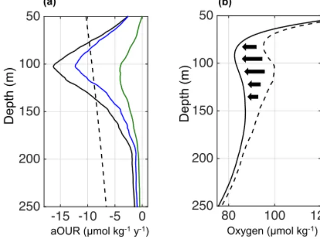
Figure 9. (a) Depth profile of the apparent oxygen utilization rate (aOUR, µmol kg−1yr−1)for the Atlantic as published from Karstensen et al. (2008; dashed black line). The oxygen consump- tion profile due to low-oxygen eddies referenced for the SOMZ region (solid black line) and the separation into CEs (blue) and ACMEs (green). The solid black line in(b)represents the observed mean vertical oxygen profile of all profiles within the SOMZ against depth, whereas the dashed black line represents the theoretical ver- tical oxygen profile in the SOMZ without the dispersion of low- oxygen eddies. Naturally due to the dispersion of negative oxygen anomalies, the observed values (black line) are lower than the theo- retical oxygen concentrations in the SOMZ without eddies (dashed black line). The impact of the dispersion of low-oxygen eddies on the oxygen budget in the depth of the shallow oxygen minimum zone is also indicated by the thick black arrows.
eddies are observed such as the interruption of the diurnal migration of zooplankters (Hauss et al., 2016).
We observed low-oxygen cores only in ACMEs (also known as submesoscale coherent vortices in D’Asaro, 1988, and McWilliams, 1985, or intra-thermocline eddies in Kos- tianoy and Belkin, 1989) and CEs but not in normal anti- cyclonic rotating eddies. In fact the ML base in normal an- ticyclonic eddies is deeper than the surroundings, bending downward towards the eddy center as a consequence of the anticyclonic rotation. Therefore the normal anticyclones cre- ate a positive oxygen anomalies when using depth levels as a reference. However, when using density surfaces as a ref- erence, the anomalies disappear. Moreover, normal anticy- clonic eddies have been found to transport warm and salty anomalies (Schütte et al., 2016a) along with the positive oxy- gen anomaly, which is very different from the ACMEs (and CEs) with a low-oxygen core.
The ETNA is expected to have a rather low population of long-lived eddies (Chaigneau et al., 2009; Chelton et al., 2011), we could identify 234 CEs and 18 ACMEs per year in the ETNA with a radius > 45 km and a tracking time of more than 3 weeks. For the eddy detection we used an algorithm based on the combination of the Okubo–Weiß method and a modified version of the geometric approach from Nencioli et al. (2010) with an adjusted tracking for the ETNA (for more
information see Schütte et al., 2016a). Schütte et al. (2016a) found an eddy-type-dependent connection between SLA and SST (and SSS) signatures for the ETNA that allowed a de- tection (and subsequently closer examination) of ACMEs.
Because of weaker SLA signatures, the tracking of ACMEs is rather difficult due to the small signal-to-noise ratio (not the case for the CEs) and automatic tracking algorithms may fail in many cases. Note that all tracks of ACMEs and CEs shown in Fig. 4 were visually verified. Similar to Schütte et al. (2016a), we derived “dead-zone” eddies surface com- posites for SST, SSS (not shown here) and Chl (Fig. 6). It revealed that the existence of an ACMEs is very associated with low SST (and SSS) but also with high Chl (see also sin- gle maps in Karstensen et al., 2015). Analyzing jointly SLA, SST and Chl maps we found that ACMEs represent a non- negligible part of the eddy field (32 % normal anticyclones, 52 % CEs, 9 % ACMEs; Schütte et al., 2016a).
It has been shown (Fig. 4) that the low-oxygen eddies in the ETNA could be separated into two different regimes:
north and south of 12◦N. The eddies north of 12◦N are gen- erally generated along the coast and in particular close to the headlands along the coast. Schütte et al. (2016a) suggested that CEs and normal anticyclones north of 12◦N are mainly generated from instabilities of the northward directed along- shore Mauritania Current (MC), whereas the ACMEs are most likely generated by instabilities the Poleward Under- current (PUC). However, the detailed generation processes need to be further investigated. The low-oxygen eddies south of 12◦N do not originate from a coastal boundary upwelling system. Following the trajectories it seems that the eddies are generated in the open ocean between 5 and 7◦N. In general, the occurrence of oxygen-depleted eddies south of 12◦N is rather astonishing, as due to the smaller Coriolis pa- rameter closer to the Equator the southern eddies should be more short-lived and less isolated compared to eddies further north. In addition, the generation mechanism of the southern eddies is not obvious. The eddy generation could be related to the presence of strong tropical instabilities in that region (Menkes et al., 2002; von Schuckmann et al., 2008). How- ever, in particular the generation of ACMEs is complex and has been subject of scientific interest for several decades al- ready (D’Asaro, 1988; McWilliams, 1985). The low strati- fication of the eddy core cannot be explained by pure adia- batic vortex stretching alone as this mechanism will result in cyclonic vorticity, assuming that f dominates the rela- tive vorticity. Accordingly, the low stratification in the eddy core must be the result of some kind of preconditioning in- duced by for example upwelling, deep convection (Oliver et al., 2008) or diapycnal mixing near the surface or close to boundaries (D’Asaro, 1988) before eddy generation takes place (McWilliams, 1985). D’Asaro (1988), Molemaker et al. (2015) and Thomsen et al. (2015) highlight the impor- tance of flow separation associated with headlands and sharp topographical variations for the generation of ACMEs. This notion is supported by the fact that low potential vorticity
signals are usually observed in the ACMEs (D’Asaro, 1988;
McWilliams, 1985; Molemaker et al., 2015; Thomas, 2008).
The low potential vorticity values suggest that the eddy has been generated near the coast as – at least in the tropical lati- tudes – such low potential vorticity values are rarely observed in the open ocean. These theories seem to be well suitable for the ACME generation north of 12◦N but do not entirely explain the occurrence of ACMEs south of 12◦N. However, more research on this topic is required.
Because we expect “northern” and “southern” eddies to have different generation mechanisms and locations and be- cause they have different characteristics we discuss them sep- arately. The core of the eddies generated north of 12◦N is characterized by less saline and cold SACW (Schütte et al., 2016a) and thereby forms a strong hydrographic anomaly against the background field. In contrast, the core of the eddies generated south of 12◦N does not show any sig- nificant hydrographic anomalies. However, a low-oxygen core in eddies is observed in both regions, indicating that the combination of the isolation of the eddy core and the high productivity in the eddy surface waters also occurs in both regions. The oxygen content decreases on average by about 0.19±0.08 µmol kg−1d−1in an ACME and by about 0.10±0.12 µmol kg−1d−1 in an CE, based on 504 oxygen measurements in CEs and ACMEs. Note that these appar- ent oxygen utilization rates (aOUR) are in the range of re- cently published aOUR estimates for CEs (Karstensen et al., 2015) and ACMEs (Fiedler et al., 2016), which are based on single measurements in “dead-zone” eddies. In partic- ular for CEs we take that as an indication that no signif- icant trend in aOUR exists. An important point regarding the method and the associated inaccuracies in deriving the aOURs is the initial coastal oxygen concentration, which is highly variable in coastal upwelling regions (Thomsen et al., 2015). In addition one should mention that the relative mag- nitude of eddy-dependent vertical nutrient flux, primary pro- ductivity and associated oxygen consumption or nitrogen fix- ation/denitrification in the eddy cores strongly varies among different eddies because of differences in the initial water mass in the eddies’ core, the eddies’ age and isolation and the experienced external forcing (in particular wind stress and dust/iron input).
However, the mean oxygen profiles from the eastern boundary and inside of all CEs and ACMEs (Fig. 3b) indi- cate no pronounced oxygen difference beneath 250 m depth.
The largest anomalies have been observed in the eddy cores at around 100 m depth (Fig. 8). As a result of the dynamic structure, the core water mass anomalies of the ACMEs are more pronounced than the one of the CE (Karstensen et al., 2016) and consequently the oxygen anomalies are stronger.
This is supported by the differences in the oxygen anomaly based on the measured plus reconstructed and the measured oxygen values. The reconstruction of oxygen values assumes a complete isolation of the eddy core. The left side of Fig. 8a, which includes the reconstructed oxygen values, features a