Computer simulation of pedestrian dynamics at high densities

Computer simulation of pedestrian dynamics at high densities

Inaugural - Dissertation

zur

Erlangung des Doktorgrades

der Mathematisch-Naturwissenschaftlichen Fakult¨at

der Universit¨at zu K¨oln

vorgelegt von

Christian Eilhardt

aus Rosenheim

K¨oln

2014

Berichterstatter: Prof. Dr. Andreas Schadschneider

Prof. Dr. Armin Seyfried

Tag der m¨ undlichen Pr¨ ufung: 17. Oktober 2014

ACKNOWLEDGEMENTS

During the last few years, I met, worked with, and have been inspired by far too many people to explicitly mention all of them here. I am grateful for the support!

First of all, I want to thank my supervisor Prof. Andreas Schadschneider for introducing me to the exciting topic of pedestrian dynamics and giving me the op- portunity to write this dissertation. I have learned a lot in our discussions. His advice and guidance have been invaluable to my work.

I am very grateful to Prof. Armin Seyfried for acting as my second supervisor and also for welcoming me into his working group and supporting me when the continuation of my dissertation was uncertain. I also want to thank Mohcine Chraibi for his advice and for many interesting and constructive discussions about my work and beyond.

Thanks to all of my colleagues at Cologne University and J¨ ulich Research Centre, in particular to Stefan Nowak and Ulrich Kemloh, for providing a pleasant and con- structive working atmosphere and for interesting discussions about physics and the world in general.

For proofreading, I want to thank Kanut Kirches and Jonathan Weskott. Your effort made this work better. I am grateful to my friends for their understanding and sympathy when I – once again – worked late into the night.

Finally, I want to express my deepest thanks to my family for their unwavering

support at all times. This work would not have been possible without the love and

care of my wonderful wife, Gesa. Thank you!

ABSTRACT

Computer simulation of pedestrian dynamics at high densities by

Christian Eilhardt

The increasing importance and magnitude of large-scale events in our society calls for continuous research in the field of pedestrian dynamics. This dissertation investi- gates the dynamics of pedestrian motion at high densities using computer simulations of stochastic models.

The first part discusses the successful application of the Floor Field Cellular Au- tomaton (FFCA) in an evacuation assistant that performs faster than real-time evac- uation simulations of up to 50, 000 persons leaving a multi-purpose arena. A new interpretation of the matrix of preference improves the realism of the FFCA simula- tion in U-turns, for instance at the entrance to the stands.

The focus of the second part is the experimentally observed feature of phase sep- aration in pedestrian dynamics into a slow-moving and a completely jammed phase.

This kind of phase separation is fundamentally different to known instances of phase

separation in e.g. vehicular traffic. Different approaches to modeling the phase sep-

aration are discussed and an investigation of both established and new models of

pedestrian dynamics illustrates the difficulties of finding a model able to reproduce

the phenomenon. The Stochastic Headway Dependent Velocity Model is introduced

and extensively analyzed, simulations of the model evolve into a phase-separated

state in accordance with the experimental data. Key components of the model are

its slow-to-start rule, minimum velocity, and large interaction range.

KURZZUSAMMENFASSUNG

Computersimulation von Fußg¨angerdynamik bei hohen Dichten von

Christian Eilhardt

Die zunehmende Bedeutung und die wachsenden Besucherzahlen von Großver- anstaltungen in unserer Gesellschaft erfordern kontinuierliche Forschung im Bereich der Fußg¨angerdynamik. Diese Dissertation untersucht das Verhalten von Fußg¨anger- str¨omen bei hohen Dichten mit Computersimulationen stochastischer Modelle.

Der erste Teil der Arbeit beschreibt die erfolgreiche Anwendung des ‘Floor Field Cellular Automaton’ (FFCA) Modells in einem Evakuierungsassistenten, der Simu- lationen von bis zu 50.000 Personen schneller als in Echtzeit durchf¨ uhrt. Eine neue Interpretation der Pr¨aferenzmatrix des Modells verbessert den Realismus der Simu- lation in U-Turns, zum Beispiel vor Mundl¨ochern in einem Stadion.

Der Schwerpunkt des zweiten Teils ist die experimentell beobachtete Separation

in eine sich langsam bewegende und eine stehende Phase in Fußg¨angerstr¨omen bei

hohen Dichten, die grundlegend anders ist als z.B. die aus dem Fahrzeugverkehr

bekannte Phasenseparation. Eine Untersuchung von etablierten und neuen Modellen

der Fußg¨angerdynamik veranschaulicht die Schwierigkeiten, ein geeignetes Modell zur

Reproduktion des Ph¨anomens zu finden. Schließlich wird das ‘Stochastic Headway

Dependent Velocity’ (SHDV) Modell vorgestellt und umfassend analysiert. Simula-

tionen des Modells entwickeln einen phasenseparierten Zustand in ¨ Ubereinstimmung

mit den experimentellen Daten. Die wichtigsten Komponenten des Modells sind seine

slow-to-start-Regel, Mindestgeschwindigkeit und große Wechselwirkungsreichweite.

TABLE OF CONTENTS

ACKNOWLEDGEMENTS . . . . iii

ABSTRACT . . . . iv

KURZZUSAMMENFASSUNG . . . . v

CHAPTER I. Introduction . . . . 1

1.1 General concepts of pedestrian dynamics . . . . 2

1.1.1 Collective phenomena . . . . 2

1.1.2 Basic quantities in pedestrian dynamics . . . . 4

1.1.3 Density concepts . . . . 5

1.1.3.1 Global density . . . . 5

1.1.3.2 Θ-density . . . . 5

1.1.3.3 Voronoi density . . . . 6

1.1.4 Fundamental diagram . . . . 7

1.1.5 Trajectories . . . . 8

1.2 Experimental situation . . . . 9

1.2.1 Experiment ‘Bergische Kaserne’ . . . . 9

1.2.2 BaSiGo experiments . . . . 13

1.3 Modeling of pedestrian dynamics . . . . 13

1.3.1 Classification of modeling approaches . . . . 13

1.3.2 Initial conditions . . . . 15

1.3.2.1 Homogeneous initial condition . . . . 16

1.3.2.2 Inhomogeneous initial condition . . . . . 16

1.3.2.3 Random initial condition . . . . 17

1.3.2.4 Almost homogeneous initial condition . 17 II. Floor Field Cellular Automaton (FFCA) . . . . 19

2.1 Floor fields . . . . 20

2.2 Transition probabilities . . . . 22

2.3 Matrix of preference . . . . 22

2.4 Friction . . . . 23

2.5 FFCA algorithm overview . . . . 24

2.6 Possible model extensions . . . . 25

2.7 Modified matrix of preference . . . . 26

III. The Hermes project . . . . 28

3.1 Simulation speed . . . . 31

3.2 Different modes of evacuation . . . . 32

3.3 Validation . . . . 33

3.3.1 Fundamental diagram . . . . 33

3.3.2 Entrance to the stands . . . . 36

3.4 Routing . . . . 40

3.4.1 Shortest paths . . . . 41

3.4.2 Quickest paths . . . . 42

3.4.3 Stochastic routing . . . . 43

3.5 Distribution of evacuation times . . . . 46

3.6 Outlook . . . . 48

IV. Modeling of phase separation in pedestrian dynamics . . . . 50

4.1 Phase separation in driven transport models . . . . 51

4.2 Floor Field Cellular Automaton . . . . 54

4.3 Generalized Centrifugal Force Model . . . . 56

4.4 Adaptive Velocity Model . . . . 58

4.5 Simple CA Model . . . . 60

4.5.1 Model definition . . . . 60

4.5.2 Results . . . . 63

4.6 Distance Based Velocity Model . . . . 66

4.6.1 Model definition . . . . 66

4.6.2 Results . . . . 69

V. Stochastic Headway Dependent Velocity Model . . . . 71

5.1 Model definition . . . . 71

5.2 Initial condition . . . . 74

5.3 Fundamental diagram . . . . 76

5.4 Velocity distribution . . . . 79

5.5 Trajectories . . . . 80

5.6 Order parameter . . . . 84

5.6.1 Definition . . . . 84

5.6.2 Results . . . . 88

5.7 Model modifications and parameter sensitivity . . . . 89

5.7.1 Stopping probability . . . . 89

5.7.2 Continuous time limit . . . . 94

5.7.2.1 Parallel update . . . . 97

5.7.2.2 Random sequential update . . . 101

5.7.3 Minimum velocity . . . 106

5.7.4 System size . . . 110

5.8 Phase separation density regime . . . 114

5.9 Phase separation mechanism . . . 119

5.10 Requirements for phase separation . . . 120

5.11 Outlook . . . 123

VI. Conclusion . . . 124

APPENDICES . . . . 126

A. Additional plots from the SHDV model . . . 127

B. Publications and talks . . . 130

B.1 Publications . . . 130

B.2 Talks . . . 131

BIBLIOGRAPHY . . . . 132

ERKL ¨ ARUNG . . . . 142

CHAPTER I

Introduction

The world population steadily increases and more people than ever before live in urban areas. Large-scale events grow in both magnitude and frequency and even daily commuting travel may exhibit high-density crowds at train stations. Clearly a detailed understanding of the underlying dynamics of pedestrian crowds should be pursued in order to appropriately design locations where high densities are expected and adequately act in case of an emergency. Crowd disasters such as the tragic catastrophe during the Love Parade 2010 in Duisburg (Germany) where 21 people died and many more were injured further illustrate that improving the safety of large- scale events is an important research topic.

The development of elaborate models and computer simulations is an established

method to describe phenomena in many complex systems including pedestrian dy-

namics. Computer simulations are used to predict evacuation times and ideally also

critical areas where dangerously high densities might be reached and accidents are

more likely to happen. Realistic models require careful calibration and validation with

the help of empirical or experimental data. Because every model is necessarily limited

in scope, occasionally, some detail of the experimental data cannot be described by

existing models. While this does not generally invalidate the established models, new

knowledge might be gained by developing a model that is capable of reproducing the

new phenomenon. To gain insight into such an experimentally observed but not yet understood phenomenon, a typical approach is trying to find the simplest system that exhibits the relevant behavior (‘minimal model’). After the simple system has been understood, it can be expanded into a more complex and potentially more realistic system.

This dissertation is structured as follows: The rest of this chapter introduces gen- eral concepts of pedestrian dynamics, gives a short overview of common modeling approaches, and discusses the experimental data relevant for this work. In Chap- ter II, the established Floor Field Cellular Automaton [1, 2, 3, 4] (FFCA) as well as a new modification of the model are presented. The application of the FFCA within the Hermes project [5, 6] is discussed in Chapter III. As part of an evacu- ation assistant for a multi-purpose arena the FFCA performs faster than real-time evacuation simulations of up to 50, 000 persons. Chapter IV explains the notion of phase separation that has been observed in one-dimensional pedestrian motion at high densities. Several established and novel models are examined as to whether they can successfully reproduce the effect. In Chapter V, a new one-dimensional model is defined and extensively analyzed. The Stochastic Headway Dependent Velocity (SHDV) Model is able to reproduce the experimentally observed phase separation in pedestrian dynamics. A discussion of the model characteristics that are required for this kind of phase separation concludes the chapter. Finally, the contribution of this work is summarized and possible future work is proposed in Chapter VI.

1.1 General concepts of pedestrian dynamics

1.1.1 Collective phenomena

The dynamics of pedestrian motion gives rise to a multitude of self-organization

phenomena that are briefly presented here. A more detailed discussion can be found

e.g. in [7, 8, 9].

• Lane formation [10, 11, 12, 13, 14]: Bidirectional pedestrian movement, e.g.

in a corridor, causes distinct lanes to emerge in which pedestrians only move in one direction. The order and quantity of these lanes dynamically varies.

The formation of lanes reduces interactions with pedestrians moving in the opposite direction and thus leads to higher velocities. While cultural bias toward walking on a specific side influences this effect, it is not required to observe lane formation in pedestrian counterflow.

• Jamming: In high-density situations where many people want to move through a bottleneck limiting the flow, jamming (clogging) occurs [1, 15, 16]. Another example for jamming is counterflow at very high densities where pedestrian moving in opposite directions completely hinder each others movement (dead- lock) [14, 17].

• Oscillations at bottlenecks [10, 11, 18]: Counterflow at bottlenecks leads to an oscillating direction of flow through the bottleneck.

• Faster-is-slower effect [8, 19]: A stronger desire

of a crowd of pedestrians to leave a room or building e.g. during an evacuation leads to a reduced flow.

• Freezing-by-heating effect [8, 20]: In pedestrian counterflow, larger fluctuations lead to a transition from movement in lanes to a deadlock.

• Patterns at crossings: Intersecting pedestrian streams can form patterns such as diagonal stripes in which pedestrians move in the same direction with the same velocity [12, 15] or short-lived roundabouts [7, 8, 21, 22]. Recently performed

1In models, this is typically represented by increasing the desired velocity and reducing cooper- ation.

experiments

investigate whether the flow through a crossing can be increased by encouraging or enforcing the roundabout motion.

1.1.2 Basic quantities in pedestrian dynamics

In addition to the qualitative characteristics described above, a thorough study of pedestrian dynamics also requires quantitative investigation. The basic quantities describing pedestrian motion are briefly introduced here.

• The velocity v of a pedestrian is straightforwardly defined as the traveled dis- tance over time or more precise as the derivative of the traveled distance with respect to the time. An actual measurement necessarily records the average velocity over a short period of time.

• The average flow

J during a time interval T is defined as the number of pedes- trians N passing a measurement line during the time interval:

J = N

T . (1.1)

• The density ρ is in general given by the number of pedestrians N within a measurement area of size A:

ρ = N

A . (1.2)

This simple definition is difficult to employ in a meaningful way because the fluctuations in the measurement can be of the same order of magnitude as the density itself. To analyze microscopic behavior, the measurement area should be small. Consider e.g. a measurement area of approximately the size of a pedestrian. The number of pedestrians inside is either 0 or 1 and fluctuations

2The experiments have been performed within the BaSiGo project briefly discussed in Sec- tion 1.2.2. The analysis of the results is ongoing.

3The precise notation for the average would behJi; in the following the brackets are omitted to simplify the notation.

play an important part. If, on the other hand, the measurement area is large, the fluctuations are much smaller. However, the density can only be measured as an average over the macroscopic measurement area. Section 1.1.3 briefly discusses a few other possible density definitions.

1.1.3 Density concepts

As discussed, the density heavily fluctuates in naive measurements. To prevent these fluctuations, other density concepts can be used. A thorough discussion of different measurement methods can be found in [23].

1.1.3.1 Global density

The simplest way to define the density is by considering the whole experimental (or simulation) setup. The density is given by the number of people over the total area, equivalent to the naive definition with the largest possible measurement section.

Using the global density precludes a microscopic analysis. It is, however, still useful for gaining macroscopic insights. The global density is an easy-to-implement and thus natural choice for computer simulations where it can also be used as an easily adjustable parameter.

1.1.3.2 Θ-density

To reduce fluctuations, the density in a measurement section at time t can be defined as

ρ(t) = P

i=1

Θ

(t)

L (1.3)

where L is the length of the measurement section, N the total number of agents, and

Θ

(t) = L

(t)

x

(t) (1.4)

Figure 1.1: Definition of Θ. The shaded region is the measurement section.

the fraction of space between the pedestrians i and i + 1 which is inside the measure- ment section, see Figure 1.1. The Θ-density [24, 25] that can then be assigned to an individual pedestrian i is defined as the average of all ρ(t) with t ∈ [t

, t

].

1.1.3.3 Voronoi density

The Voronoi density concept is based on Voronoi diagrams [26] and has been adapted to the analysis of pedestrian dynamics in [27]. Each point in space is assigned to a Voronoi cell A

associated with a specific pedestrian i such that every point inside the cell is closer to the corresponding pedestrian than to any other pedestrian.

The density ρ

of a single point (x, y) in space is given by A

with A

such that (x, y) ∈ A

. The density inside an arbitrarily small measurement area A is then given as the integral

ρ = 1 A

Z

A

dA ρ

. (1.5)

The Voronoi measurement method allows to reduce the size of the measurement area without increasing the resulting scatter [13, 28, 29] and thus improves the investigation of pedestrian dynamics on a microscopic scale.

The local/individual (Voronoi) density of a pedestrian in a one-dimensional system can easily be calculated by taking the inverse of the average distance to the person in front and behind,

ρ

= 2

d

+ d

(1.6)

where d

denotes the distance between pedestrian i and pedestrian i+1, measuring

from the center of each person. Note that this line density measures pedestrians per meter instead of the two-dimensional pedestrians per square meter.

1.1.4 Fundamental diagram

The fundamental diagram is one of the most important quantities to characterize the behavior of pedestrians, or traffic flow in general. In the classical formulation it depicts the flow as a function of the density. Because velocity v, flow J, and density ρ are not independent but linked by the hydrodynamic relation

J = ρ · v , (1.7)

it can also be presented as velocity vs. density or velocity vs. flow. The fundamental diagram is often referred to as the most basic observable in pedestrian dynamics and used as a tool for the calibration of computer simulation models that describe pedestrian motion [3, 30, 31].

The precise form of the pedestrian fundamental diagram is a heavily discussed topic. An often cited study of fundamental diagrams has been done by Weidmann [32].

Experimentally measured fundamental diagrams are affected by many factors such as the cultural background of participants [33, 34], psychological factors like the pedes- trian’s motivation [35], or the type of traffic [36]. Another important influence is the difference between unidirectional and bidirectional flow [9, 37, 38, 39]. Unfortunately, the exact experimental conditions have not always been documented in sufficient de- tail which is understandable considering that the importance of some effects has only been discovered after the experiments have been performed.

As outlined in Section 1.1.3, the density (and the velocity as well) can be measured

in many different ways. The characteristics of the measurement method influence the

resulting fundamental diagram [40]. This should be considered when the fundamental

diagram is used to calibrate models.

Two variants of the fundamental diagram for one-dimensional movement are pri- marily used in this work, namely the global fundamental diagram which uses velocity and density values averages over the whole system and the local fundamental dia- gram. The latter uses the local density defined in Section 1.1.3.3 and the individual velocity. Note that the lack of averaging leads to a very large number of data points as each pedestrian contributes one data point for each timestep in a simulation (or for each frame in experimental data).

1.1.5 Trajectories

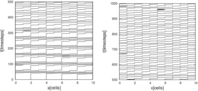
The dynamics in a one-dimensional system can be visualized using a space-time plot that depicts the trajectories of individual pedestrians. Typical trajectories of the Stochastic Headway Dependent Velocity (SHDV) Model developed in this work (see Chapter V) are given in Figure 1.2. The left image shows local trajectories zoomed

Figure 1.2: Trajectories of the SHDV model: local (left) and global (right).

in to cover only a small part of the system that, incidentally, corresponds to the size

of the measurement area of the experimental data discussed in Section 1.2.1. The

right image shows global trajectories covering the whole simulated course

. Each line corresponds to one pedestrian moving from left to right and from bottom to top.

The vertical parts of the lines correspond to jams: Time passes but the position of the pedestrian does not change. One advantage of studying trajectories instead of e.g. the fundamental diagram is that they contain the complete information of the dynamics and allow to gain further microscopic insights.

1.2 Experimental situation

To allow insights into pedestrian dynamics, either empirical data or data from laboratory experiments has to be studied. A typical approach to gather quantitative data is the analysis of video footage [41, 42, 43, 44, 45, 46]. This can be done

‘by hand’ or automatically by using e.g. the software PeTrack

[45, 46] to extract precise trajectories of individual pedestrians. The latter, however, requires special markers to detect the exact pedestrian positions and can at this point only be used in laboratory experiments. Quantitative data of pedestrian dynamics can be used to calibrate mathematical or computer simulation models aiming to describe pedestrian motion [42, 47, 48, 49, 50] and search for ‘laws of nature’ characterizing pedestrian dynamics.

1.2.1 Experiment ‘Bergische Kaserne’

For this work, one series of experiments is of particular importance. In 2006, Seyfried et al. [25, 39] performed experiments with up to 70 pedestrians that ex- amine one-dimensional (single-file) pedestrian movement. A similar experiment had already been executed in 2005 [51] and evaluated manually to obtain the fundamen- tal diagram. The participants were instructed to ‘move normally’ and not allowed

4A larger version of this image can be found in Appendix A.

5PeTrack has been used in both the Hermes and BaSiGo projects.

Figure 1.3: Experimental setup [25, 39].

to overtake. The experimental setup depicted in Figure 1.3 had a length of approxi- mately 26 m including a 4 m long measurement section in which the pedestrian tra- jectories have been measured by automatically tracking the pedestrian heads [45, 46].

The positions of pedestrians outside the measurement section have not been cap- tured. Several runs with different numbers of pedestrians and thus different density have been conducted.

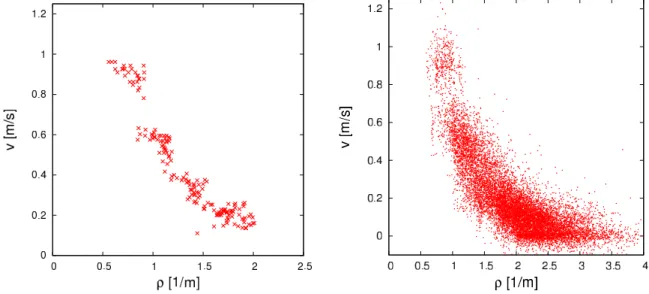
The fundamental diagram can be obtained using either the Θ-density [24, 25] dis- cussed in Section 1.1.3.2 or the Voronoi [27] (individual) density. Both variants are depicted in Figure 1.4. The negative velocities in the local fundamental diagram come

Figure 1.4: Fundamental diagram of the experimental data using the Θ-density (left) and the Voronoi density (right).

from the backward-moving heads of standing pedestrians. This effect results from not

tracking the center of mass, but the head of each pedestrian. The local fundamental

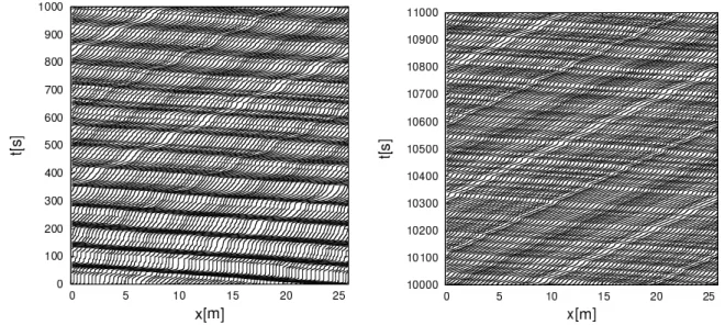
Figure 1.5: Experimental trajectories for N = 45 (left) and N = 70 (right).

diagram contains much higher densities. This can be explained by considering that the local fundamental diagram contains unaveraged data and the distance between two heads can be much smaller than between two persons. The macroscopic funda- mental diagram on the other hand averages over multiple pedestrians as discussed in Section 1.1.3.2.

The resulting trajectories of two typical runs are shown in Figure 1.5 (left) as a space-time plot. At very high densities, a separation into phases with standing pedestrians (vertical lines) and phases with moving pedestrians can be observed.

The velocity in the moving phase can be obtained by estimating the slope of the trajectories, it is about 0.15

and thus much smaller than the free-flow velocity, which is about 1.2

. From vehicular traffic a similar effect is known, namely a separation into a jammed and free-flowing phase. This will be discussed in more detail in Section 4.1. Small (backward) movements in the trajectories come from the head movement of standing pedestrians.

The existence of a jam in the system raises the question whether the system con-

tains multiple jams or the observed jam in the measurement section is the only jam in

the experimental setup. The trajectories are compatible with both scenarios because

Figure 1.6: Experimental velocity distribution [25].

the experimental data only extends over the small time-scale of 140 s and spatial scale of 4 m. This also prevents judging the stability of the empirical phase separation, it is unclear whether the phases remain separate for longer timescales. The existence of additional jams would be an indication that jams might be forming and decaying dynamically. Even though it has not been formally documented, the experimenters assume

that there was probably only one jam in the system. To analyze the phase separation of high-density pedestrian traffic, one has to study microscopic quantities (trajectories). It does not suffice to study the fundamental diagram which not neces- sarily contains information about the microscopic characteristics of a system. A more detailed analysis of the observed phase separation will be conducted in Chapters IV and V by comparing the experimental data to computer simulations.

The velocity distribution of the experimental data is given in Figure 1.6 for several density intervals. At high densities, it exhibits a double peak structure with one maximum at 0

and the other at about 0.1

, depending on the density. This suggests a coexistence of moving and standing pedestrians and can also be interpreted

6The goal of the experiment was to obtain a precise fundamental diagram. The very specific question about the number of jams in the system during a few high-density runs arose during the evaluation of the data, after the experiments had been performed.

as an indication of a minimum velocity.

1.2.2 BaSiGo experiments

The project BaSiGo [52] – Safety and Security Modules for Large Public Events

is funded by the German Federal Ministry of Education and Research. The goal of the project is to improve the evaluation and planning of mass events using a modular approach. One aspect of BaSiGo is the realization of large-scale experiments with up to 1000 participants.

For this work only one of the experiments conducted within the BaSiGo project is relevant, namely an almost exact replication of the experiment discussed in Sec- tion 1.2.1. The sole difference is that during the new experiment the whole experimen- tal setup has been covered by the camera grid which allows to extract the complete set of trajectories instead of only capturing a subset due to the confined measurement section. The new data allows to also consider global experimental trajectories and thus check whether there is indeed only one jam in the system. Unfortunately, the analysis of the raw data leading to the extraction of the trajectories is not yet fin- ished. Therefore the quantitative results of the new experiment are not incorporated into this work. The visual impression during the experiment

, however, suggests that there is indeed only one jam in the high-density system at any time.

1.3 Modeling of pedestrian dynamics

1.3.1 Classification of modeling approaches

An enormous number of different models has been used to describe pedestrian motion, therefore any attempt to list the numerous different approaches will probably

7in German: Bausteine f¨ur die Sicherheit von Großveranstaltungen

8The author was part of the team responsible for the planning and execution of the experiments and therefore able to observe this particular experiment live from a well-suited vantage point.

remain incomplete. Nevertheless, this work presents a possible classification based on basic characteristics of pedestrian models. A more detailed discussion can be found in e.g. [53]. For all of the properties discussed below, there are models that do not belong to either pure category but can be placed somewhere in between.

• Macroscopic models describe a system as a whole, typically using aggregated quantities such as density and flow. Microscopic models on the other hand describe the motion of individual agents and track their individual properties such as position and velocity; they also allow to personalize the agents by using different parameter values for different agents. Mesoscopic models include features of both macroscopic and microscopic models.

• Variables such as time, position, or velocity can either take integer (discrete) or real (continuous) values. An important advantage of discrete models is the efficiency in computer simulations. However, in some situations the limited resolution in contrast to continuous models can be problematic. Some models such as the Stochastic Headway Dependent Velocity (SHDV) Model discussed in Chapter V use a mix of discrete and continuous variables.

• In force-based models, the dynamics is defined in analogy to Newtonian me- chanics, agents are accelerated by ‘social’ forces. The behavior of agents in rule-based models is governed by a set of rules based on the state of the agent, its neighborhood, and possibly other factors as well. Again, some models use a mixed approach.

• In models with deterministic dynamics, the evolution of a system depends only

on the starting configuration. In stochastic models, agents in the same situ-

ation can behave differently, the dynamics is governed by probabilities. Some

models combine deterministic dynamics with an additional external noise.

The two most commonly used model classes are force-based models and cellular au- tomata (CA). Microscopic force-based models [10, 30, 48, 54, 55] are usually defined in a continuous geometry and use deterministic dynamics; CA models [1, 53, 56, 57, 58]

are microscopic, discrete, rule-based, and usually stochastic.

The discrete space used in CA models can be realized in multiple ways. The simplest and most popular lattice consists of square cells that typically have a size of 0.4 × 0.4 m

[32]. In models utilizing the von-Neumann neighborhood agents are allowed to move to the four non-diagonal neighbors [1]; the Moore neighborhood allows agents to move to all eight neighbors including the adjacent diagonal cells [58].

Another choice for CA models is to use a hexagonal lattice [59, 60, 61, 62]. An advantage of the hexagonal lattice is its improved isotropy. However, as the vast majority of buildings contains mainly right angles, for many simulations the square lattice is a more natural choice.

1.3.2 Initial conditions

Experimental initial conditions are usually difficult to control and therefore only known approximately. The participants can e.g. be instructed to distribute evenly in an experimental area, yet even in the best case the distribution is only nearly homogeneous. Simulations, in contrast, can use precisely defined initial conditions which allow to exactly reproduce their results.

In the following, typical starting configurations for periodic one-dimensional sim-

ulations are discussed. After a sufficiently long simulation time, many models reach

a stationary state that is independent from the initial condition. Depending on the

model and the parameter choice there may be several distinct stationary states that

the model can converge to, e.g. a homogeneous stationary state at low densities and

an inhomogeneous stationary state at high densities. Additionally, for applications

such as evacuation simulations or replication of experimental results it is also inter-

esting to consider the non-stationary state. Pedestrian experiments might not last long enough to ensure the convergence to a stationary state.

Initial conditions for two-dimensional simulations can be defined similarly. They will not be discussed in detail because for the two-dimensional simulations discussed in this work the initial distribution of agents is relatively unimportant in comparison to other factors determining the simulation results as will be discussed in Section 3.5.

1.3.2.1 Homogeneous initial condition

One possible initial condition is a homogeneous state in which all agents are spaced out evenly in the simulation area. If the model does not include some kind of stochas- tic influence it will typically stay in the homogeneous state in which it started. Note that models with discrete space such as CA models can in general not use a truly homogeneous initial condition. Consider for example a simulation with two agents and an area of five cells. In that case it is impossible to homogeneously distribute the agents. Models with continuous space, on the other hand, can easily implement this.

1.3.2.2 Inhomogeneous initial condition

Alternatively, the system can start in an inhomogeneous state, e.g. a megajam.

This is especially easy to implement for CA models: Assuming a total of N agents

in the simulation, the first N cells are occupied and the other cells are empty. For

space-continuous models either the size of an agent or a minimum distance between

point-like agents has to defined. The distance between agents in the simulation is then

set accordingly. Depending on the details of the model, this distance can either be a

well-defined quantity or not. For simulations with inhomogeneous initial conditions

and less than maximum density both discrete and continuous models feature a single

larger distance between two agents in the system, namely between the end of the

megajam and its beginning.

1.3.2.3 Random initial condition

The agents can be distributed randomly in the system. For CA models this is very straightforward: Every agent gets assigned to a random empty cell which is then occupied and blocked for other agents. For pedestrian models with continuous space, random initial conditions work well for relatively empty systems but can be problematic when the density is close to the maximum allowed density.

Assuming that each agent has a finite size

, overlapping has to be considered.

A straightforward idea is to place every agent at a random position such that the distance to the neighboring agents is big enough to avoid overlapping. However, at some point there might not be enough space between any two adjacent agents to allow the placement of the next agent. This becomes clear for the extreme case of considering the maximum possible density

. To allow the placement of every agent, the headway of each agent has to be equal to the agent size. A truly random distribution of agents however can and most likely will lead to headways that are larger than the agent size but not twice as large, meaning that no other agent can be placed in between. Due to the ’wasted’ space at least one agent cannot be placed at all. There are some methods

to avoid this problem, but there is no obvious way to transfer the random distribution from a CA model to space-continuous models.

1.3.2.4 Almost homogeneous initial condition

The final starting configuration discussed here is intended for space-continuous models. It is designed to be very similar to the experimental initial condition and resembles an ‘almost homogeneous’ state, which is achieved via a two-step process:

First the agents are distributed homogeneously. Then each agent’s position is shifted

9The same argument can be made for point-like agents that have to respect a minimum distance.

10For simplicity’s sake the system size is assumed to be a multiple of the agent size; the same argument is valid for a more general system size.

11One approach is to randomly distribute headways instead of positions.

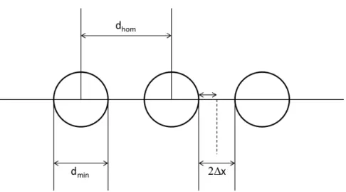
Figure 1.7: Almost homogeneous initial condition after the first step. In the second step each agent is shifted by up to ∆x.

a little according to a Gauss-distributed random variable. The Gauss-distribution is cut off at 2σ in such a way that overlapping of agents is impossible, see Figure 1.7.

The maximum distance ∆x which an agent can be shifted to either side is equal to half of the free space in between two adjacent agents:

|∆x| ≤ d

− d

2 , (1.8)

where d

is the headway or distance between the homogeneously spaced agents and d

is the size of an agent or, depending on the model, the minimum distance between point-like agents. This means the agents are indeed ‘almost homogeneously’

distributed, resulting in a realistic starting configuration.

CHAPTER II

Floor Field Cellular Automaton (FFCA)

The Floor Field Cellular Automaton (FFCA) [1, 2, 3, 4] is a microscopic, agent- based model. Space is partitioned into small non-overlapping cells which can either be empty or occupied by a pedestrian or an obstacle such as a wall. The exclusion principle is enforced: No cell can be occupied by more than one pedestrian. The size of one cell corresponds to the space requirement for a single person. A common value for the maximum density in highly crowded areas is 6.25 persons per square meter which leads to a typical cell size of 0.4 × 0.4 m

[32]. In each timestep t all pedestrians are updated in parallel. Since a reaction to the motion of other agents is only possible in the next timestep t + ∆t, the size of a timestep ∆t can be identified with the reaction time of a pedestrian. A typical choice is ∆t = 0.3 s which is of the same order of magnitude as the reaction time [1].

The rule-based dynamics of the model are defined by the transition probabili- ties p

to neighboring cells including the cell currently occupied by the pedestrian in consideration. As discussed in Section 1.3.1, there are several possibilities regard- ing the choice of the neighborhood. The most common ones are the von-Neumann neighborhood used in this work (Figure 2.1) and the Moore neighborhood.

These transition probabilities are in general determined by three factors: the

desired direction of motion, the interaction with other pedestrians and the interaction

Figure 2.1: Definition of the transition probabilities p

in the von-Neumann neigbor- hood.

with the infrastructure. For this purpose the model uses two discrete floor fields S

and D

.

2.1 Floor fields

The static floor field S

contains the information about the preferred direction of motion. It does not change in time but is calculated for each lattice site at the beginning of the simulation. It can be interpreted as a potential and describes the shortest distance to the destination site which typically corresponds to an exit. It is possible to have multiple destination cells. For complex geometries the static floor field is usually calculated with a flooding algorithm such as the Dijkstra algorithm [63].

The dynamic floor field D

transforms the long-ranged interaction between

agents into a local interaction with memory. It represents a virtual trace created by

moving pedestrians and corresponds to the tendency of pedestrians to follow other

(moving) pedestrians. The dynamic floor field is inspired by the process of chemo-

taxis which is e.g. responsible for the formation of ant trails [64]. At the start of

a simulation, the field has a value of zero on each site (ij), D

= 0. This value

increases by one whenever a pedestrian leaves the site. The increase does not affect

the leaving pedestrian in the next timestep in order to avoid a negative feedback loop

by preventing the agent from being drawn backwards by its own forward movement.

20

40

60 20

40 60

0 2 4 6

20

40

60

10

20

30 10

20 30

0 10 20 30

10

20

30

Figure 2.2: Dynamic floor field (left) and static floor field (right) during the final stage of the simulation of a large room with a single door [2].

Due to the dynamic floor field the FFCA features dynamic transition probabilities that depend on the history of the simulation.

The dynamic floor field can only have non-negative integer values, it can therefore

be loosely interpreted as a bosonic field in the following sense: The non-negative

integer value of the dynamic floor field at a given cell can be interpreted as the

number of bosons on this cell. The model dynamics then leads to varying numbers

of bosons at each cell at different timesteps. These bosons are unrelated to quantum

statistics and quantum mechanics but help visualizing the update procedure. The

increase of the dynamic floor field triggered by a moving agent then corresponds to

the creation of a boson. Additionally, the bosonic field is subject to diffusion and

decay processes. At the beginning of each timestep, every boson has a probability δ

to decay, leading to D

→ D

− 1. Every remaining boson has a diffusion probability

α to move to a random neighboring cell. This leads to a diluting and widening trace

and determines the effective interaction range: Except for local interaction via the

exclusion-principle, an agent can only interact with another agent if one of the agents

is influenced by a boson that the other agent created. The range of the interaction

therefore corresponds to the average distance a boson travels via the diffusion process

before it decays. A small decay probability and a big diffusion probability allow a

boson to travel relatively far and thus lead to a large interaction range.

2.2 Transition probabilities

The unnormalized transition probabilities (weights) p b

of the standard FFCA model for the movement of an agent to the site with relative coordinates (i, j ) are given by

b

p

= exp(k

S

) · exp(k

D

) · ξ

(2.1) where the parameters k

and k

are coupling constants which control the influence of the floor fields S and D. The factor ξ

ensures that movement is only possible to allowed sites. It prevents movement to sites that are occupied by either a pedestrian or an obstacle,

ξ

=

 

 

 



0, (i, j) empty 1, (i, j) blocked.

(2.2)

The normalized transition probabilities p

are given by

p

= N · p b

= N · exp(k

S

) · exp(k

D

) · ξ

(2.3)

where the factor

N = 1

P

ij

p b

(2.4) assures the normalization P

ij

p

= 1 of the transition probabilities.

2.3 Matrix of preference

The matrix of preference is a way to encode the preferred direction of motion of

the pedestrians. It is a 3 x 3 matrix whose entries modify the transition probabilities

depending on the direction of the movement. For the von Neumann neighborhood,

only five entries are different from zero:

M =



 

 



0 M

0 M

M

M

0 M

0



 

 

 . (2.5)

When the Moore neighborhood is used, the diagonal matrix entries corresponding to diagonal movement are also nonzero

. The transition probabilities p

including the matrix of preference are given by

p

= N · exp(k

S

) · exp(k

D

) · ξ

· M

. (2.6)

In many cases it is sufficient to use the static and dynamic floor fields to describe the behavior of the simulated pedestrians and the matrix of preference is not necessary.

This is equivalent to setting all matrix entries to M

= 1 in which case the matrix of preference does not influence the model dynamics.

2.4 Friction

Due to the parallel update in the FFCA it is possible for two or more pedestrians to choose the same target cell. This is called a conflict. The simplest solution to a conflict is to randomly choose one of the agents which is allowed to move and let the other agents stand still for the timestep. However, a more realistic behavior of the pedestrians at high densities e.g. in a bottleneck can be obtained by introducing friction [65, 66].

Friction provides a probability µ for each conflict cell that none of the conflicting pedestrians move to the chosen destination, see Figure 2.3. With probability 1 − µ

1Their values can actually be related to observable quantities such as the average velocities and their fluctuations [1].

Figure 2.3: Friction prevents the movement of conflicting agents with probability µ.

one pedestrian is allowed to move to the target cell while the others are forbidden to move. The moving pedestrian is chosen randomly from the conflicting agents.

Friction can be interpreted as a kind of local pressure between agents that results in agents disrupting each others movement such that with probability µ all conflicting agents remain in their cell.

More intuitively, friction can be interpreted as nonverbal communication between conflicting pedestrians which takes a little time. As an example, consider two pedes- trians who want to walk through a door and arrive at the same time. They might look at each other briefly, then one of them moves through the door and the other one follows. On the other hand, both pedestrians might try to move simultaneously and block each other for a short time: friction.

2.5 FFCA algorithm overview

In each timestep the following steps are performed in parallel for each agent:

• Calculate diffusion and decay of the dynamic floor field.

• Calculate the transition probabilities to the cells with relative coordinates (i, j).

• Choose a target cell using these transition probabilities.

• Resolve potential conflicts and move the agents who are allowed to move.

• Increase the value of the dynamic floor field according to the moving agents.

Typical parameter values for the diffusion probability α, the decay probability δ, the coupling constants k

and k

of the static and dynamic floor field, respectively, and the friction parameter µ are given in Table 2.1. The specific values of the parameters generally depend on the scenario that is analyzed.

parameter value

α 0.2

δ 0.2

k

2.5

k

2.0

µ 0.3

Table 2.1: Parameter values for the FFCA model.

2.6 Possible model extensions

There are several possibilities to extend the FFCA model:

• Higher velocities (v

> 1): Pedestrians are allowed to move more than one cell in each timestep. This leads to an increased interaction range and a more complex pedestrian behavior such as possible crossings of trajectories within a single timestep [65, 67].

• Politeness factor: An additional factor p

= exp(−k

N

) is added to the probabilities in Equation (2.3), where N

is the number of nearest neighbors on site (i, j). This leads to a suppression of motion into the direction of crowded areas [3, 58].

• Smaller cell sizes: In order to represent the infrastructure of a building in more detail, smaller cells are used. For 20 × 20 cm

cells each pedestrian occupies 2 × 2 cells [65, 67].

• Inertia: Inertia effects suppress abrupt changes in the direction of motion [1, 68].

To that end an additional factor

p

=

 

 

 



exp(k

), direction of motion changes

1, direction of motion remains unchanged

is added to the probabilities in Equation (2.3). The value of the parameter k

determines the strength of the inertia effect.

• Wall repulsion: An additional factor p

= exp k

· min(D

, d

)

can be included in Equation (2.3) to describe the interaction between walls and pedes- trians [68, 69]. k

denotes the coupling constant and thus the strength of the interaction, D

is the range of the wall potential and d

is the distance of the agent from the nearest wall.

This is by no means a complete list of possible model extensions. There is a multi- tude of further generalizations and modifications of the floor field cellular automaton model, such as defining an additional vector floor field that describes the force act- ing on a pedestrian [70, 71] or using a different underlying lattice structure (e.g. a hexagonal lattice [59, 60, 61, 62]).

2.7 Modified matrix of preference

This section proposes a new interpretation of the matrix of preference presented in Section 2.3 which can be used as a tool to locally modify transition probabilities.

The modified matrix of preference can be employed to more realistically describe pedestrian movement in a U-turn. This will be discussed in Section 3.3.2.

By linking the matrix of preference to a specific cell, any agent occupying that

cell is influenced by the matrix of preference. In principle each cell – instead of

each pedestrian – can have its own matrix of preference in addition to the static

and dynamic floor field, leading to a lot of freedom to influence the movement of

pedestrians in a given geometry. An interesting choice is using a matrix of preference that has trivial entries

for all directions except for one, e.g. downwards,

M =



 

 



0 1 0

1 1 1

0 exp(k

) 0



 

 

 . (2.7)

The entry exp(k

) increases the transition probability for a movement downwards as if the static floor field in the target cell were increased by one: The probability to move downwards is given by

p

= N · exp(k

S

) · exp(k

D

) · M

· ξ

(2.8)

where the indices ‘1,0’ denote the downwards direction of movement according to the definitions in Figure 2.1 and Equation (2.5). M

thus corresponds to the nontrivial matrix entry exp(k

). Equation (2.8) can then be simplified to

p

= N · exp(k

S

) · exp(k

D

) · exp(k

) · ξ

(2.9)

= N · exp(k

(S

+ 1)) · exp(k

D

) · ξ

(2.10)

which is equal to the transition probability without a matrix of preference but with a static floor field that is increased by one in the target cell. It is not possible to directly change the static floor field in a way equivalent to the above change.

2A matrix of preference with all entries equal to 1 does not change the transition probabilities.

CHAPTER III

The Hermes project

Figure 3.1: ESPRIT arena [72].

Hermes [5, 6] was an interdisciplinary three-year project funded by the German

Federal Ministry of Education and Research in the program ‘Research for Civil Secu-

rity’ and successfully finished in 2011. A main goal of the project was to increase the

safety of people participating in or attending big events in large buildings like sport

stadiums by developing a proof of concept for an evacuation assistant that is capable

Figure 3.2: Structure of the evacuation assistant. Graphic courtesy of Ulrich Kem- loh [73].

of forecasting an evacuation of up to 50,000 pedestrians faster than real-time

. The ESPRIT arena (Figure 3.1) in D¨ usseldorf, Germany has been chosen as the site of the proof of concept.

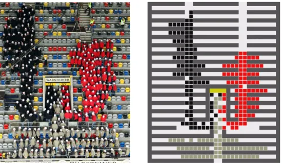
Figure 3.2 shows the general structure of the evacuation assistant. The geometry of the multifunctional arena as well as the data from automated person counting and the safety and security management system, which tracks the available and unavailable exit routes, are used as input for computer simulations performed on a local computer cluster. These simulations are faster than real-time, meaning that a forecast over 15 minutes can be calculated in one to two minutes, depending on the model. The simulations predict evacuation times as well as high-risk areas, that is areas where high densities and congestion occur. The simulation results are displayed in the user interface, called communication module, which is shown in Figure 3.3. It can be accessed by the decision-makers who can then adapt the positioning of security personnel in order to divert pedestrian flows and avoid high-risk situations. A second

1The evacuation assistant can in principle also be used for outdoor events. However, in that case different approaches to some technical aspects of the project are required.

Figure 3.3: User interface of the evacuation assistant.

use case of the evacuation assistant is in the planning phase of an event. The usually automatically gathered input data can be entered or changed manually which allows the creation and detailed analysis of evacuation plans for user-created scenarios.

The evacuation assistant includes several computer models, namely the force-

based Generalized Centrifugal Force Model (GCFM) [30], the Network Model Vi-

sum [74], the cellular automaton model PedGo [75] and the Floor Field Cellular

Automaton (FFCA, see Chapter II) [1, 2, 3]. The geometry input data needs to be

provided in two different formats for the continuous and the discrete models and is

generated in a semi-automatic fashion. This work focuses on simulations performed

with the FFCA.

3.1 Simulation speed

The FFCA simulations use only a small fraction of the available computing power as most of the processors of the Hermes-workstation are reserved for simulation with the GCFM. A big advantage of cellular automaton models such as the FFCA is their computation speed. Due to the discrete nature of the FFCA and its resulting lower spatial and time resolution it is much faster than the continuous GCFM. The area of interest, roughly one quarter of the whole arena, has a size of about 15, 000 m

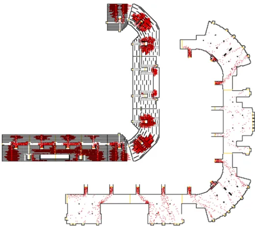
, which are approximately 93, 000 cells. A simulation with 12, 000 agents, shown in Figure 3.4, takes 30 s on a standard computer. The simulated time is 15 min and corresponds to the typical time for evacuation. This means that the simulation runs about 30 times faster than real-time. The simulation time of the FFCA could of

Figure 3.4: Simulation snapshots of the stands (top left) and the promenade (bottom

right) of the ESPRIT arena.

course be optimized further, trivially by using a faster computer, but also by runtime optimization of the program code or by parallelization. This is however not necessary as the FFCA is already fast enough, the evacuation assistant only slightly benefits from a further speed-up of the model. A distinct advantage of the FFCA model with regards to applications is that it runs faster than real-time without being reliant on a local computer cluster.

3.2 Different modes of evacuation

The simulations feature two different evacuation modi. Routine egress on the one hand happens regularly after every event when the audience leaves the building. This kind of egress is strongly influenced by unknown factors and diverse pre-movement time

, varying motivations to leave the arena and hard-to-predict route choices (see Section 3.4) depending on the mood and the preferred method of transportation of the pedestrian. Routine egress is therefore difficult to simulate. Emergency evac- uations on the other hand happen very rarely. In the case of an emergency, the evacuation process is much more straightforward and therefore easier to simulate.

Each pedestrian has a high motivation to leave the arena, often using the shortest path outside. The distribution of individual pre-movement delay is much narrower and corresponds to the distribution of reaction times – once the stadium announcer asks for evacuation, everybody starts to move as quickly as possible.

Independent of the mode of evacuation there are factors such as the route choice behavior of pedestrians leaving the arena that are not necessarily well-known. This is discussed in further detail in Section 3.4.

2Time an individual spends between the end of the event and beginning to leave the building.

The influence of the pre-movement time has been analyzed in [76].

3.3 Validation

It is a well-established fact that the FFCA features typical collective phenomena as described in Section 1.1.1. However, a quantitative approach to model calibration allows for more accurate quantitative predictions. This has been discussed in more detail in [77].

The validation of the ESPRIT arena simulations without any data from emergency evacuations was one of the challenges of the project. In addition to the data from routine egress, there is experimental data from simpler geometries with a much lower number of participants but better control over their behavior. This data is also used in the validation process which is performed in various steps.

To get reasonable simulation results for complex geometries such as the ESPRIT arena, one first has to understand the basic geometries, namely corridors, bottlenecks and corners. A comparison of simulation results with experimental data of the one- dimensional fundamental diagram will be used in Section 3.3.1 to perform a basic calibration of the FFCA parameter values. The movement of agents around corners within the framework of the FFCA has been studied in [78] and [79]. The next step is to validate the model for intermediate geometries by comparing simulation results to experiments. To this end a vomitory

is considered which connects the stands of the arena to the promenade leading to the exits. A detailed analysis of simulations and experiments using this geometry will be conducted in Section 3.3.2.

3.3.1 Fundamental diagram

The first part of the FFCA calibration is based on the fundamental diagram introduced in Section 1.1.4. The single-file nature of movement in the experiment

‘Bergische Kaserne’ discussed in Section 1.2.1 justifies using a one-dimensional variant of the floor field model. The corridor has a length of L = 26 m which corresponds

3in German: ‘Mundloch’.

to

= 65 cells with periodic boundary conditions. Three different variants of the model are used for simulations: the standard FFCA with v

= 1, a variant with v

= 2, and an improved model which includes a politeness factor as discussed in Section 2.6. Higher speeds in the simulation are defined in the simplest possible way: Each person determines a destination cell at a maximum distance of 2 cells.

Conflicts

are resolved analogously to the model with v

= 1. Either both agents are denied movement due to friction or one randomly chosen pedestrian is allowed to move.

Figure 3.5: Comparison of empirical and simulated fundamental diagrams for three variants of the FFCA. The simulation density is given by the global den- sity ρ =

.

The first analysis of the simulation results utilizes the global density definition ρ =

where N is the number of pedestrians. This is a natural choice for simulations because it allows to treat the density as an easily adjustable parameter. Figure 3.5 shows the comparison of the empirical data with simulation results for the three

4Conflicts are possible in the one-dimensional model because a backwards motion is in principle possible. However, they are very unlikely and the influence of friction is thus negligible in a one- dimensional geometry.

parameter v

= 1 (standard) v

= 1 (improved) v

= 2 (standard)

α 0.3 0.2 0.1

δ 0.2 0.2 0.2

k

2.5 3 1.8

k

3.5 3 4.8

k

0 4.5 0

µ 0 0 0

Table 3.1: Parameter values for simulations using the global density.

variants. The parameter values are fitted by eye and given in Table 3.1. The standard model with v

= 1 does not give a good agreement with the experimental data.

However, both model extensions lead to a considerable improvement.

To analyze the influence of the measurement method, the local Θ-density defini- tion introduced in Section 1.1.3.2 is utilized in the simulation. Thus both experiment and simulation measure density and flow in the same way. Figure 3.6 shows the sim- ulated fundamental diagrams for the v

= 2 model and for two different parameter sets given in Table 3.2. The simulation with the parameter set optimized for the

parameter v

= 2 (global) v

= 2 (local)

α 0.1 0.1

δ 0.2 0.2

k

1.8 4

k

4.8 4.8

k

0 6.5

µ 0 0

Table 3.2: Parameter values for simulations using the Θ-density.

global density measurement does not result in a good agreement with the empirical

data. The simulation that uses the parameter set optimized for the local Θ-density

measurement on the other hand matches the experimental data well. Using the lo-

cal density measurement in the simulation, fluctuations become an issue because the

length of the measurement section (4 m) corresponds to only 10 cells. In order to

reduce the resulting scatter, the size of the simulated system is increased by a factor

of 10. The simulation of the original system size shown in the inset of Figure 3.6

Figure 3.6: Experimental data and simulated fundamental diagrams of the v

= 2 model variant with different parameter sets. The blue circles denote the parameter set which is optimized for the global density definition whereas the parameters of the green triangles are optimized for the local measurement.

features a much larger fluctuation, however the agreement with the empirical data is still good. Simulations with the model variant including politeness factor show similar results.

The measurement method in the simulation has a strong influence on the simu- lation results. Consequently, one should always aim to use the same measurement methods in simulations as in the experiments that are used to calibrate the corre- sponding model. This has been discussed in detail in [23].

3.3.2 Entrance to the stands

The stands of the arena are connected to the promenade which in turn leads to

the exits. The entrance to the stands is designed in the form of a vomitory, see

Figure 3.7. Within the scope of the Hermes project an experiment [80] has been

conducted to investigate the pedestrian flow in the proximity of the vomitory. The