Validated force-based modeling of pedestrian dynamics
130
0
0
Volltext
(2)
(3)
(4)
(5)
(6)
(7)
(8)
(9)
(10)
(11)
(12)
(13)
(14)
(15)
(16)
(17)
(18)
(19)
(20)
(21)
(22)
(23)
(24)
(25)
(26)
(27)
(28)
(29)
(30)
(31)
(32)
(33)
(34)
(35)
(36)
(37)
(38)
(39)
(40)
(41)
(42)
(43)
(44)
Abbildung

+7
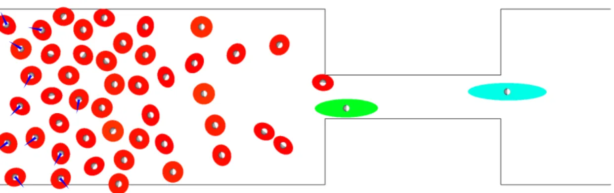
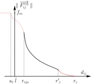
![Figure 2.5: Schematic representation of the collision detection technique (CDT), which is an important component in the CFM [130], to manage collisions and mitigate overlapping among pedestrians](https://thumb-eu.123doks.com/thumbv2/1library_info/3697444.1505853/50.918.156.764.128.890/schematic-representation-collision-detection-technique-collisions-overlapping-pedestrians.webp)
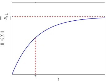
![Figure 2.6: Simulations with the CFM without the CDT compared with empirical data from [63]](https://thumb-eu.123doks.com/thumbv2/1library_info/3697444.1505853/51.918.316.626.160.471/figure-simulations-cfm-cdt-compared-empirical-data.webp)
![Figure 4.1: Off-line trajectory detection with PeTrack [4]. Left: The trajectory of the detected pedestrian shows strong swaying](https://thumb-eu.123doks.com/thumbv2/1library_info/3697444.1505853/67.918.168.801.107.342/figure-trajectory-detection-petrack-trajectory-detected-pedestrian-swaying.webp)
ÄHNLICHE DOKUMENTE
Snow slab avalanches result from a se- quence of fracture processes including (i) failure ini- tiation in a weak layer underlying a cohesive snow slab, (ii) the onset of
ABSTRACT: A velocity servocircuit for retracting the access mechanism of a disk storage drive independently of the nor mal position servo, including a summing amplifier connected
This unequal geographic distribution and the positive correlation between the number of physicians and health care costs is often seen as evidence for demand inducement and
SBE 37 Seabird Electronics SBE37 recording temperature and conductivity (optionally pressure SBE 37 P) PIES Pressure Inverted Echo Sounder (optionally with current meter
The repeats since 1993 are part of a long-term assessment of changes in the transports of heat, salt and fresh-water through 48 ° N that continued with this
Simultaneously, data was recorded from three linear position transducers [T-FORCE (version 2.3, T-FORCE Dynamic Measurement System, ERGOTECH Consult- ing, Murcia, Sp), Tendo
Simultaneously, data was recorded from three linear position transducers [T-FORCE (version 2.3, T-FORCE Dynamic Measurement System, ERGOTECH Consult- ing, Murcia, Sp), Tendo
The temperature dependence of the velocity from the present and recently reported [5] hypersonic data are summarized in Table 2 together with ultrasonic data [4]. All the
