1
Calculation of entropy-dependent thermodynamic properties of fluids at high pressure with computer simulation
Inaugural-Dissertation zur Erlangung des Doktorgrades
der Mathematisch-Naturwissenschaftlichen Fakultät der Universität zu Köln
Simin Yazdi Nezhad aus Mashhad, Iran
Köln 2016
For my parents and for my brothers
3
Berichterstatter:
Prof. Dr. U. K. Deiters Insitut für Physikalische Chemie
Universität zu Köln
Priv. Doz. Dr. T. Kraska Insitute für Physikalische Chemie
Universität zu Köln
Tag der mündlichen Prüfung: 20.01.2016
First of all, I would like to express my deep gratitude to my advisor Prof. Dr. Ulrich K.
Deiters, for his enduring guidance and tremendous help in my research and the writing of this thesis.
I would like to express my gratitude to Dr. Tomas Kraska for his support of this project.
I am also grateful to all my friends and colleagues with whom I had a enjoyable time during my PhD study.
I am indebted to my parents for raising me and supporting me in all my life.
5
Notation
A rotation matrix
E energy
Ekin kinetic energy
Epot potential energy
F Helmholtz free energy
f force
G Gibbs free energy
g(r) radial distribution function
h Planck’s constant
kB Boltzmann’s constant
L length of simulation box
m mass
N number of particles
NA Avogadro’s constant
P probability
p pressure
p momentum
Q partition function
r distance
r location vector
rc cut-off radius of the pair potential
rhc hard-core radius
R universal gas constant
S entropy
Sr residual entropy
T temperature
u(r) pair potential function
U internal energy
∆U difference of internal energy
V volume
Vf molar free volume
Vidf free volume in an ideal gas
W work
x Monte Carlo shift parameter
Z compressibility factor
Z configuration integral
"0 permittivity of vacuum
" depth of Lennard-Jones potential
ρ number density
σ diameter of a molecule
σhs hard-sphere diameter
ξ random number in range (0,1)
λ thermal wavelength
µ chemical potential
φ Euler angle
θ Euler angle
ψ Euler angle
ω molecular orientation
∗ denotes reduced variables
〈· · · 〉 ensemble average
Subscripts
c cut-off
hs hard sphere
kin kinetic
m molar
pot potential
p derivative at constant pressure
r residual
T derivative at constant temperature V derivative at constant volume
Acronyms
CPU Central Processing Unit
CSJS-LJ Carnahan–Starling+Jacobsen-Stewart Lennard-Jones equation of state
LJ Lennard-Jones
KN-LJ Kolafa–Nezbeda Lennard-Jones equation of state
mBWR1-LJ modified Benedict–Webb–Rubin Lennard-Jones equation of state mBWR2-nLJ modified Benedict–Webb–Rubin Lennard-Jones chain equation of state
MC Monte Carlo
MD Molecular Dynamics
vdw van der Waals
Zusammenfassung
Es ist lange bekannt, dass es Zusammenhänge zwischen der Entropie und dem freien Volumen eines Fluids gibt. Neuerdings wurde vor allem bei Simulationen üssiger Me- talle über Korrelationen zwischen der Entropie und der Diusionskonstante berichtet.
Bei manchen Fluiden gibt es zudem einen Zusammenhang zwischen der residuellen Entropie und dem Verschiebungsparameter bei Monte-Carlo-Simulationen. Da dieser Parameter während einer Simulation ohnehin berechnet wird, erönet sich damit die Möglichkeit, entropieabhängige thermodynamische Gröÿen ohne Mehraufwand zu be- stimmen.
Es ist jedoch noch nicht klar, in welchen Klassen von intermolekularen Potentialen diese Beziehung angewandt werden könnte und welche Dichte oder Temperatur gewählt werden muss. Ein formaler statistisch-thermodynamische Beweis ist auch noch nicht erbracht worden.
In dieser Arbeit wurde eine neue, eziente Methode zur Berechnung der residu- ellen Entropie entwickelt. Zum Vergleich wurde die Einfügungsmethode von Widom verwendet.
Die potentielle Energie des Systems wurde als Summe aller Zweikörper-Wechselwir- kungspotentiale berechnet. Es wurden periodische Randbedingungen verwendet, um Oberächeneekte zu minimieren.
Die Simulation wurde für Ein- und Zweizentren-Moleküle durchgeführt, wobei zwi- schen den Zentren Mie-6 Potentiale, insbesondere Lennard-Jones-Potentiale, und Harte- Kugel-Potentiale angenommen wurden.
Im Rahmen dieser Arbeit wurde die Verbindung zwischen der residuellen Entropie und dem Monte-Carlo-Verschiebungsparameter in Flüssigkeiten mit hoher Dichte als Polynom zweiten Grades bestätigt. Das Anwendungsgebiet ist zu niedrigen Dichten durch einen Perkolationsübergang begrenzt.
Zum Vergleich wurden Entropien mit der Theorie von Scheraga, mit der radialen
Verteilungsfunktion nach der Theorie von Baranyai und schlieÿlich mit Hilfe von Zu-
standgleichungen für Harte-Kugel-Fluide bzw. Lennard-Jones-Fluide ermittelt.
.
Abstract
It has been long known that there is a connection between the entropy and the free volume of uids. More recently, it has been shown that there is a correlation between the entropy and the diusion constant in liquid metals by simulation.
In some uids, a relevancy between the residual entropy and Monte Carlo shift parameter was discovered. Because this parameter is calculated during simulation in any case, it is possible to calculate the other thermodynamic properties that are connected to the entropy without additional cost.
However, it is not yet clear in which classes of intermolecular potentials this rela- tionship could be applied and which density or temperature must be chosen. A formal statistical-thermodynamic proof is also still missing.
In this work, a new ecient method was developed to calculate the residual en- tropy. For comparison, the Widom test particle insertion method was used to calculate chemical potentials.
The potential energy of a system was calculated as a sum of the two-body interaction potentials. Moreover, periodic boundary conditions were used to minimize surface eects.
Simulations were performed for single- and two-center molecules. For the site- site interactions, Mie potentials, especially Lennard-Jones potentials and hard-sphere potentials were adopted.
In this work, the connection between the residual entropy and the Monte Carlo shift parameter in uids at high densities was obtained as a second-order polynomial equation. The application range of this equation is limited at low densities by percola- tion.
For comparison, the entropy was determined by the theory of Scheraga, from the
radial distribution function by the theory of Baranyai and nally with help of equations
of state for Lennard-Jones and hard-sphere uids.
1 Introduction 19
2 Statistical Thermodynamics 25
2.1 Principles of Monte Carlo simulation . . . . 26
2.1.1 Concept of ensembles . . . 26
2.1.2 Boltzmann factors and ensemble averages . . . 27
2.1.3 Monte Carlo simulation (MC) . . . 28
2.1.4 Hit-or-miss Monte Carlo . . . 28
2.1.5 The Metropolis method . . . 29
2.2 Trial moves . . . . 32
2.2.1 Translational moves . . . 32
2.2.2 The maximum displacement . . . 33
2.2.3 Orientational move of rigid molecules . . . 33
2.2.4 Calculation of maximum rotation angle . . . 35
2.2.5 Volume change in N p T ensemble . . . 36
2.2.6 Calculation of the maximum expansion factor . . . 36
2.3 Periodic boundary conditions . . . . 36
2.4 Minimum image convention . . . . 38
2.5 Intermolecular Interactions . . . . 39
2.6 Calculation of thermodynamic properties . . . . 39
2.6.1 The effect of kinetic energy in Monte Carlo simulation . . . 39
2.6.2 Residual thermodynamic properties . . . 40
2.6.3 Calculation of residual internal energy . . . 40
2.6.4 Calculation of residual pair virial . . . 41
2.6.5 Calculation of virial pressure in N V T ensemble . . . 41
2.6.6 Calculation of the virial pressure in N p T ensemble . . . 42
2.6.7 Calculation of packing density . . . 43
2.6.8 Long-range corrections . . . 43
2.7 Sitesite potentials . . . . 43
2.7.1 The Lennard-Jones potential . . . 43
2.7.2 Correction of the Lennard-Jones potential . . . 45
2.7.3 The Lorentz-Berthlot mixing rules . . . 45
2.7.4 The Mie potential . . . 45
10
CONTENTS 11
2.7.5 Correction of the Mie-potential . . . 46
2.7.6 Calculation of Mie force . . . 46
2.7.7 Correction of Mie potential pair virial . . . 47
2.7.8 Calculation of virial compression factor . . . 47
2.7.9 The hard-sphere Potential . . . 47
2.7.10 Calculation of Carnahan-Starling compressibility factor . . . 48
2.8 Radial distribution function . . . . 48
2.8.1 Radial distribution function in Lennard-Jones fluids . . . 48
2.8.2 Radial distribution function in hard-sphere fluids . . . 49
2.9 Calculation of entropy-related properties . . . . 52
2.9.1 The chemical potential . . . 52
2.9.2 Homogeneous functions and entropy . . . 55
2.9.3 Widom insertion method . . . 56
2.9.4 Alternatives routes to the entropy . . . 56
2.9.5 Scheraga’s theory . . . 57
2.9.6 The estimation of entropy from radial distribution function . . . 58
2.10 Percolation theory . . . . 59
2.10.1 Introduction . . . 59
2.10.2 The percolation problem . . . 59
2.11 Reduced Units . . . . 62
3 Simulation Programs 65 3.1 Details of the computer simulation program mc++ . . . . 66
3.2 Random number generator . . . . 69
3.3 Equilibration and production phase . . . . 70
3.4 The inner hard core of Lennard-Jones sites . . . . 70
3.5 The computer systems . . . . 71
4 Results and discussion 73 4.1 The test of the computer simulation program . . . . 74
4.2 Calculation of the residual entropy for LJ uids . . . . 79
4.2.1 1-center Lennard-Jones argon . . . 79
4.2.2 Lennard-Jones argon dimers . . . 81
4.2.3 Linear Lennard-Jones argon trimers . . . 83
4.2.4 Non-linear Lennard-Jones argon trimers . . . 84
4.2.5 1-center Mie-potential argon . . . 86
4.2.6 Mie-potential argon dimers . . . 92
4.2.7 Linear Mie-potential argon trimers . . . 99
4.2.8 Non-linear Mie-potential argon trimers . . . 100
4.2.9 Dimer CH
3-CH
3. . . 101
4.3 Calculation of the residual entropy for hard-sphere uids . . . . 102
4.4 Calculation of the residual entropy for LJ uids . . . . 104
4.5 Estimating the errors . . . . 105 4.6 Calculation of the residual entropy and estimation of relative errors . 105 4.7 Calculation of the residual entropy with dierent methods . . . . 107 4.7.1 Lennard-Jones fluids . . . 107 4.7.2 Hard-sphere fluids . . . 111
5 Conclusion 117
6 Appendix 119
List of Figures
2.1 Monte Carlo calculation of
π. . . 29
2.2 Accepting or refusal of the moves in the MC simulation. . . 30
2.3 Displacement in Monte Carlo simulation. . . 31
2.4 Two dimensional periodic system. . . 37
2.5 The minimum image convention in two-dimensional system. . . 38
2.6 Argon Lennard-Jones potential . . . 44
2.7 Space distribution for the evaluation of the radial distribution function. . . 48
2.8 Bond and side percolation . . . 60
2.9 Percolation in one dimension. . . 60
2.10 Percolation in two dimensions. . . 61
2.11 Percolation in 2 dimension square lattices . . . 61
3.1 Schematic representation of the simulation program mc
++. . . 69
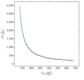
4.1 Residual chemical potential vs. molar volume for argon, T
=200 K . . . 75
4.2 Molar residual entropy vs. molar volume for argon, T
=200 K . . . 76
4.3 Molar internal energy vs. molar volume for argon, T
=200 K . . . 76
4.4 Compression factor vs. molar volume for argon, T
=200 K . . . 77
4.5 Residual chemical potential vs. molar volume for argon, T
=600 K . . . 77
4.6 Residual molar entropy vs. molar volume for argon, T
=600 K . . . 78
4.7 Molar internal energy vs. molar volume for argon, T
=600 K . . . 78
4.8 Compression factor vs. molar volume for argon, T
=600 K . . . 79
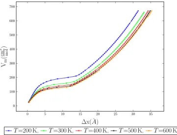
4.9 Molar volume vs. MC shift parameter for various temperatures for 1-center LJ fluid argon. . . 80
4.10 Entropy vs. MC shift parameter for 1-center LJ fluid argon . . . 80
4.11 Atom coordination of Lennard-Jones argon dimers. . . 81
4.12 Entropy vs. MC shift parameter for Lennard-Jones argon dimers . . . 82
4.13 Atom coordinates of linear Lennard-Jones argon trimers. . . 83
4.14 Entropy vs. MC shift parameter for linear Lennard-Jones argon trimers . . 84
4.15 Atom coordinates of non-linear Lennard-Jones argon trimers. . . 85
4.16 Entropy vs. MC shift parameter for non-linear LJ argon trimers . . . 86
4.17 Entropy vs. MC shift parameter for 1-center Mie-potential argon . . . 87
4.18 Entropy vs. MC shift parameter for 1-center Mie-potential argon, 30% . . . 87
4.19 Entropy vs. MC shift parameter for 1-center Mie-potential argon, accep- tance ratio 50%, T
=500 K. . . 88
13
4.20 Entropy vs. MC shift parameter for 1-center Mie-potential argon, accep-
tance ratio 30%, T
=500 K. . . 88
4.21 Entropy vs. MC shift parameter for 1-center Mie-potential argon, accep- tance ratio 50%, T
=800 K. . . 90
4.22 Entropy vs. MC shift parameter for 1-center Mie-potential argon, accep- tance ratio 30%, T
=800 K. . . 90
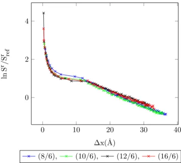
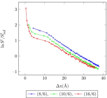
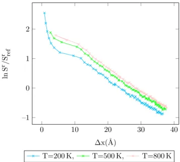
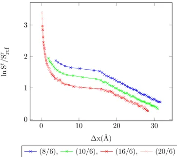
4.23 Entropy vs. MC shift parameter for 1-center Mie-potential argon (8
/6) at different temperatures, acceptance ratio 50%. . . 91
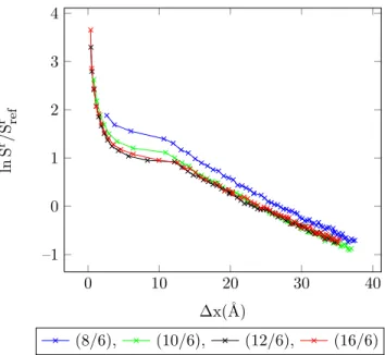
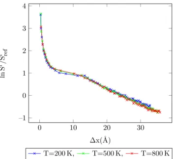
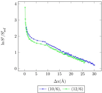
4.24 Entropy vs. MC shift parameter for 1-center Mie-potential argon (10
/6) at different temperatures, acceptance ratio 50%. . . 91
4.25 Entropy vs. MC shift parameter for 1-center Mie-potential argon (16
/6) at different temperatures, acceptance ratio 50%. . . 92
4.26 Entropy vs. MC shift parameter for Mie-potential argon dimers, accep- tance ratio 50%, T
=200 K. . . 93
4.27 Entropy vs. MC shift parameter for Mie-potential argon dimers, accep- tance ratio 30%, T
=200 K. . . 93
4.28 Entropy vs. MC shift parameter for Mie-potential argon dimers, accep- tance ratio 50%, T
=500 K. . . 94
4.29 Entropy vs. MC shift parameter for Mie-potential argon dimers, accep- tance ratio 30%, T
=500 K. . . 95
4.30 Entropy vs. MC shift parameter for Mie-potential argon dimers, accep- tance ratio 50%, T
=800 K. . . 96
4.31 Entropy vs. MC shift parameter for Mie-potential argon dimers, accep- tance ratio 30%, T
=800 K. . . 96
4.32 Entropy vs. MC shift parameter for Lennard-Jones argon dimers (8
/6) at different temperatures, acceptance ratio 50%. . . 97
4.33 Entropy vs. MC shift parameter for Lennard-Jones argon dimers (10
/6) at different temperatures, acceptance ratio 50%. . . 97
4.34 Entropy vs. MC shift parameter for Lennard-Jones argon dimers (16
/6) at different temperatures, acceptance ratio 50%. . . 98
4.35 Entropy vs. MC shift parameter for Lennard-Jones argon dimers (20
/6) at different temperatures, acceptance ratio 50%. . . 98
4.36 Entropy vs. MC shift parameter for linear Mie-potential argon trimers, T
=200 K, acceptance ratio 50%. . . 99
4.37 Entropy vs. MC shift parameter for non-linear Mie-potential argon trimers, T
=200 K, acceptance ratio 50% . . . 100
4.38 Entropy vs. MC shift parameter for CH
3-CH
3at different temperatures, acceptance ratio 50%. . . 101
4.39 Entropy vs. MC shift parameter for hs argon, acceptance ratio 50%. . . 103
4.40 Entropy vs. MC shift parameter for a hs fluid, acceptance ratio 50%. . . 103
4.41 residual entropy vs. MC shift parameter in Lennard-Jones fluids. . . 104
4.42 Entropy vs. MC shift parameter for hard-sphere argon, T
=400 K . . . 106
LIST OF FIGURES 15
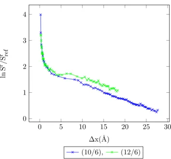
4.43 Entropy vs. MC shift parameter for Mie-potential argon dimers (10
/6), T
=200 K . . . 106 4.44 Acceptance ratio vs. Monte Carlo shift parameter for argon, T
=200 K,
V
=50 cm
3mol
−1. . . 108 4.45 Acceptance ratio vs. Monte Carlo shift parameter for argon, T
=300 K,
V
=100 cm
3mol
−1. . . 110
4.46 Acceptance ratio vs. MC shift parameter for hs argon, V
=45 cm
3mol
−1. . . 111
4.47 Acceptance ratio vs. MC shift parameter for hs argon, V
=50 cm
3mol
−1. . . 112
4.48 Acceptance ratio vs. MC shift parameter for hs argon, V
=55 cm
3mol
−1. . . 113
4.49 Acceptance ratio vs. MC shift parameter for hs argon, V
=60 cm
3mol
−1. . . 114
4.50 Acceptance ratio vs. MC shift parameter for hs argon, V
=65cm
3mol
−1. . . 115
4.51 Acceptance ratio vs. MC shift parameter for hs argon, V
=70 cm
3mol
−1. . . 116
2.1 Some microscopic and macroscopic properties . . . 26
2.2 Summary of common statistical ensemble . . . 27
3.1 The computer systems used for the simulations . . . 71
4.1 Simulation details for 1-center Lennard-Jones argon. . . 79
4.2 Begin of percolation for 1-center Lennard-Jones argon. . . 81
4.3 Simulation details for Lennard-Jones argon dimers. . . 82
4.4 Begin of percolation for Lennard-Jones argon dimers . . . 82
4.5 Simulation details for linear Lennard-Jones argon trimers. . . 83
4.6 Begin of percolation for linear Lennard-Jones argon trimers. . . 84
4.7 Simulation details for non-linear Lennard-Jones argon trimers. . . 85
4.8 Begin of percolation for non-linear Lennard-Jones argon trimers. . . 85
4.9 Begin of percolation for 1-center Mie-potential argon, T
=200 K. . . 86
4.10 Begin of percolation for 1-center Mie-potential argon, T
=500 K. . . 89
4.11 Begin of percolation for 1-center Mie-potential argon, T
=800 K. . . 92
4.12 Begin of percolation for Mie-potential argon dimers, T
=200 K. . . 94
4.13 Begin of percolation for Mie-potential argon dimers, T
=500 K. . . 95
4.14 Begin of percolation for Mie-potential argon dimers, T
=800 K. . . 95
4.15 Begin of percolation for linear Mie-potential argon trimers, T
=200 K. . . 99
4.16 Begin of percolation for non-linear Mie-potential argon trimers, T
=200 K. 100 4.17 Simulation details for CH
3-CH
3. . . 101
4.18 Start of percolation for CH
3-CH
3. . . 102
4.19 Simulation details for hard-sphere argon . . . 102
4.20 Estimates of the relative error for hard-sphere argon, T
=400 K. . . 107
4.21 Estimates of the relative error for Mie-potential argon dimers (10
/6), T
=200 K. . . 107
4.22 Results of the simulation program for argon, T
=200 K . . . 109
4.23 Calculation of the residual entropy with different EOS for argon, T
=200 K . 109 4.24 Results of the simulation program for argon, T
=300 K, V
=100 cm
3mol
−1. . 109
4.25 Calculation of the residual entropy with different EOS for argon, T
=300 K. 110 4.26 Calculation of the residual entropy with different equation of state for hard-sphere argon, V
=45 cm
3mol
−1. . . 111
4.27 Calculation of the residual entropy with different equation of state for hard sphere argon, V
=50 cm
3mol
−1. . . 112
16
LIST OF TABLES 17
4.28 Calculation of the residual entropy with different equation of state for
hard sphere argon, V
=55 cm
3mol
−1. . . 113
4.29 Calculation of the residual entropy with different equation of state for hard sphere argon, V
=60 cm
3mol
−1. . . 114
4.30 Calculation of the residual entropy with different equation of state for hard sphere argon, V
=65 cm
3mol
−1. . . 115
4.31 Calculation of the residual entropy with different equation of state for hard sphere argon, V
=70 cm
3mol
−1. . . 116
6.1 Vapour-pressure curve of argon from mBWR2-nLJ equation of state. . . 121
6.2 Acceptance ratio vs. residual entropy for argon, T
=200 K . . . 122
6.3 Acceptance ratio vs. residual entropy for argon, T
=300 K . . . 123
6.4 Radial distribution function of argon, T
=200 K . . . 124
6.5 Radial distribution function of argon, T
=300 K . . . 125
6.6 RDF of hs argon in the Percus-Yevick approximation, V
m=45 cm
3mol
−1. . . 126
6.7 RDF of hs argon in the Percus-Yevick approximation, V
m=50 cm
3mol
−1. . . 127
6.8 RDF of hs argon in the Percus-Yevick approximation, V
m=55 cm
3mol
−1. . . 128
6.9 RDF of hs argon in the Percus-Yevick approximation, V
m=60 cm
3mol
−1. . . 129
6.10 RDF of hs argon in the Percus-Yevick approximation, V
m=65 cm
3mol
−1. . . 130
6.11 RDF of hs argon in the Percus-Yevick approximation, V
m=70 cm
3mol
−1. . . 131
6.12 The results of MC
++simulation program for argon . . . 132
Chapter 1
Introduction
19
Introduction
One of the main goals of research in the eld of applied thermodynamics is the prediction of thermodynamic and transport properties of uids and their mixtures.
Among the various thermodynamic properties, knowledge of the phase behaviour of uids is particularly important for many applications. The required thermodynamic properties can be calculated in two dierent ways:
1. Empirical methods, which were generated from a large set of experimental data.
These methods are particularly suitable for application to systems for which there are many measured data.
2. Theoretical methods, which are based on statistical thermodynamic theories.
For almost half a century, computer simulation methods have been used in the re- search on liquids, particularly in scientic, engineering and industrial research. Over the previous decades, the speed of computers has rapidly increased. For this reason, computer simulation has become a very important tool for calculating the thermody- namic properties of uids.
The rst molecular simulations of liquids were performed by Metropolis on the MANIAC computer at Los Alamos [1, 2].
The main motivation of molecular simulation is the calculation of accurate proper- ties of statistical mechanical systems. Molecular simulations can be described as compu- tational statistical mechanics. Molecular simulations determine macroscopic properties with the use of computer programs. This allows the precise evaluation
1of theoreti- cal models of molecular behavior, whereas classical statistical thermodynamics are frequently restricted to the use of simplistic models.
Molecular simulation can be done in two dierent ways: molecular dynamics simu- lation (MD) and Monte Carlo simulation (MC).
Molecular dynamics simulation (MD) : as the name indicates, molecular dynamics makes it possible to obtain the dynamic properties of the system. MD uses the follow- ing steps to calculate macroscopic thermochemical properties:
É
Setting up the system in an initial conguration
É
Solving Newton's equations of motion for the system of molecules:
d
2−→r
idt
2 =−→
F
im
ii
=1, 2, 3, . . .
1with errors depending on the computer speed and size.
21 where F
i, m
i, and r
iare the force on particle i , mass, and position of particle i , re- spectively. The momenta and the molecular coordinations change according to the intermolecular forces experienced by the individual molecules [77].
É
Calculating average properties (energy, pressure, pair correlation functions) after the system has reached equilibrium.
Monte Carlo simulation (MC) : the details of the Monte Carlo simulation is presented in section 2.1.3 on page 28.
The molecular dynamics and Monte Carlo simulation methods are dierent in a several of ways:
É
Molecular dynamics simulation (MD) provides information about the time depen- dence of the properties of the system, whereas there is no temporal relationship be- tween successive Monte Carlo congurations.
É
In a Monte Carlo simulation (MC) the outcome of each trial move depends only on its immediate predecessor, whereas in molecular dynamics it is possible to predict the conguration of the system at any time in the future or indeed at any time in the past.
É
Molecular dynamics has a kinetic energy contribution to the total energy, whereas in the Monte Carlo simulation the total energy is determined directly from the potential energy function.
É
Monte Carlo simulation calculates the changes in intermolecular energy, whereas molecular dynamics uses intermolecular forces to evolve the system.
Until 1970 , computer simulation was only feasible for studies of structural and sim- ple thermodynamic properties, such as pressure, enthalpy, energy and pair correlation functions. Some properties such as entropy, Helmholtz energy and chemical potential are dicult to calculate because they are not representable as ensemble averages of mechanical properties. Today, dierent methods are available for the calculation of chemical potential and free energies, etc.:
É
The Widom test particle insertion method:
The most widely used methods for the calculation of chemical potentials, free en- ergies and etc. are based directly or indirectly on the insertion method of Widom [3].
The Widom test particle method has been used to obtain phase diagrams for pure [6, 7]
and binary mixtures [8, 9].
In this method, a new particle is added at a random location and the change in
average energy is calculated. The details of this method will be discussed in section
2.9.3 on page 56.
É
The two-ensemble method: (know as Gibbs ensemble method)
The two-ensemble method for the calculation of phase equilibria with Monte Carlo simulation was developed by Panagiotopoulos [10, 11].
A distinguishing feature of the two-ensemble method is that it entails two simulation boxes (subsystems) that are coupled to each other. The coupling between them is done in such a way as to achieve coexistence between two phases. This methode uses insertion steps to bring both ensembles to equilibrium with each other [31].
É
The grand canonical ensemble simulation:
In simulations using the grand canonical ensemble
(µ, V , T
), the calculation of chemi- cal potentials is not needed. The particle numbers are allowed to uctuate by insertions and deletions steps.
Insertion steps which add a new particle to a random location in a uid are only possible if enough place for a new particle is available. Simulation methods based on insertion steps tend to become inecient if the systems have very high densities (compressed uid, solid, etc). Moreover, they become inecient or very complicated if
the particles do not have spherical shapes.
To avoid these problems, deletion methods have been suggested (for example by Boulougouris et al. [12]). But they cause statistical problems [2022] and fall down if they are used for molecules with long-range interactions [23, 24].
É
Estimation of the entropy from radial distribution function (RDF) [64] and Scheraga theory : [52, 53]
These are two other methods to calculate residual entropy, which are explained later in detail.
There are other methods to determine chemical potentials and free energies, for example umbrella sampling [15], the method of Hoheisel and Deiters (This method is universally applicable [16], but needs a lot of time for the calculations and cannot be automatized easily) and the method of Kofke [13, 14] (that can be used along phase boundary curves), but they are used infrequently. An overview of available methods is presented in the book of Frenkel and Smit [30].
It has long been known that the entropy and the free volume of a uid are connected [17]; this had been published in 1981 by Speedy [18]. More recently, correlations between the entropy and the diusion have been reported in the simulation of liquid metals [19].
In the present work, the Monte Carlo method, combined with the Widom test
particle method, is used to calculate chemical potentials and residual entropies of the
nobel gas argon, hard-sphere argon, a dimer CH
3-CH
3. Furthermore, a new method
for computing the entropy of uids is introduced and tested, which avoids some of the
shortcomings of the Widom method.
23
The Chapter 2 gives a short introduction the statistical thermodynamic and the
principles of Monte Carlo simulation. Chapter 3 gives a description of the simulation
program and its details, and at last, Chapter 4 and Chapter 5 present the results and
the conclusion of this project, respectively.
Chapter 2
Statistical Thermodynamics
25
2.1 Principles of Monte Carlo simulation
2.1.1 Concept of ensembles
The relationship between the microscopic description of individual molecules and the macroscopic properties of a collection of molecules is a central concept in statistical mechanics [30].
The state of a macroscopic system can be specied by a few properties. For exam- ple, a pure liquid can be described completely by its mass, pressure and temperature.
However, for each macroscopic state, there exists a large number of microscopics states corresponding to it. For classical systems, the positions and momenta of all theirs constituent molecules characterize each microscopics state.
Table 2.1: Some microscopic and macroscopic properties
properties of individual molecules
properties of bulk fluid (microscopic properties) (macroscopic properties)
intermolecular force the equation of state molecular geometry internal energy
velocities heat capacity
position pressure
An ensemble of systems is a collection of various microscopics states of the system, which correspond to the single macroscopic state of the system whose properties are investigated.
As there are several ways to specify the macroscopic state of the system, various ensembles types can be dened. The commonly used ensembles are given in Table 2.2.
The ensembles in Table 2.2 can be divided into two categories. The grand canonical ensemble represents open systems in which the number of particles can be changed; the isothermal-isobaric, canonical and microcanonical ensembles are for closed systems, in which the number of particles is constant [77].
Because of the equivalence of the ensembles in the thermodynamic limit, it is pos- sible to transform between dierent ensembles [42]. The choice of the ensemble for a simulation is entirely a matter of convenience. If a system has a xed number of molecules and is kept at either constant volume and temperature or constant pressure and temperature, the best choices are isothermal-isobaric and canonical ensembles, respectively.
The most important ensembles, which are used besides the classical canonical en-
sembles in computer simulation are the grand canonical ensemble (
µ, V , T ) and the
isobaric-isothermal ensemble ( N , p, T ).
2.1. PRINCIPLES OF MONTE CARLO SIMULATION 27
Table 2.2: Summary of common statistical ensemble. Table taken from
[77
]. type of ensemble constant
variables
Z P
idescription
microcanonical N , V , E
Pi
δ(Ei−
E
) δ(EQN V Ei−E)isolated system
canonical N , V , T
Pi
e
−βEi(N,V) e−βQEi(N,V)N V T
closed isothermal system
grand canonical
µ, V , T
Pi
e
βNiµQ
N V T e−β(QEiµV T−µNi)open isothermal system isothermal-
isobaric
N , p , T
Pi
e
βp ViQ
N V T e−β(QEi+p Vi)N p T
closed isothermal-isobaric
system
In Table 2.2, Z and P
istand for the partition function and the probability of observing the i -the state, respectively.
2.1.2 Boltzmann factors and ensemble averages
The microscopic states of a canonical ensemble with N particles are not all equally probable [26]. The probability P
(i
)of a microscopic state i with the energy E
iis pro- portional to the Boltzmann factor exp
(−E
i/(kBT
)), where k
Bis the Boltzmann constant:
[27]
P
(i)∝exp
−
E
ik
BT
(2.1) The points in phase space are distributed according to a probability. Moreover, the total energy of a state is sum of the potential and the kinetic energy. Therefore Equation (2.1) can be rewritten as
P
(i) =e
−βEi(N,V)Q
N V T(2.2)
E
=〈E
kin〉+E
pot(2.3)
Q
N V T =Xi
e
−βEi(N,V)(2.4)
where Q
N V Tis the canonical partition function and acts as a normalizing factor.
From the probability distribution, the ensemble average of a property A can be calculated in the following way:
〈
A
〉ens=Xi
A
iP
i(2.5)
where
〈A
〉ensis the ensemble average of the system.
2.1.3 Monte Carlo simulation (MC)
The word Monte Carlo was coined by Metropolis because of the use of random numbers, and used for rst time in 1943 by three scientists at the Los Alamos National Laboratory in New MexicoNicolas Metropolis, John von Neumann, and Stanislaw Ulamto study the diusion of neutrons in ssionable materials [25].
The MC method can be used in dierent elds from economics or nuclear physics to the regulation of trac ow. It is a stochastic technique for studying many-body systems and for obtaining thermodynamic properties that can be expressed as an en- semble averages. The pressure and internal energy are examples of such properties.
Basic characteristics and some advantages of Monte Carlo method are :
•
Dierent types of probability distributions can be assigned to the inputs of the model.
When the distribution is known, the one that represents the best t can be chosen.
•
The use of random numbers characterizes Monte Carlo simulation as a stochastic method. The random numbers have to be independent; no correlation should exist between them.
•
Simulations provide detailed information on the model systems.
The steps in Monte Carlo simulation corresponding to the uncertainty propagation are relatively simple: [77]
1. Generating a trial conguration randomly.
2. Evaluating an acceptance criterion by calculation of the change in energy, and other properties in the trial conguration.
3. Comparing the acceptance criterion to a random number and either accepting or rejecting the trial conguration.
2.1.4 Hit-or-miss Monte Carlo: calculation of π
The naive MC technique (this method is called naive Monte Carlo because it works
with random sampling) can be used as a method of integration, for example for the
2.1. PRINCIPLES OF MONTE CARLO SIMULATION 29 evaluation of
π. This calculation can be done by nding the area of a circle of radius R . Figure 2.1 shows the circle, centred at the origin and inscribed in a square [42].
+ +
O A
B C
x y
Figure 2.1: Monte Carlo calculation of
π.
Now points are chosen randomly inside the square. Points with x
2+y
2<1 lie inside the circle. The area of the circle can then be approximately obtained from:
4
×area of circle
area of enclosing square
'4
×number of points inside the circle
total number of points (2.6) Then
πcan be computed from:
π=
4
πR2(
2R
)2 =4
×area of circle
area of enclosing square (2.7)
2.1.5 The Metropolis method
Metropolis (1953) described a new approach where instead of choosing conguration randomly from an equidistribution (naive Monte Carlo method), the conguration is chosen with the probability exp
(−E
/kBT
)(Boltzmann factor)[28]. For a system in which the potential energy depends on position, Metropolis' idea can be expressed by the following equation:
〈
A
〉=1 X
X
i=1
A
(q
i)(2.8)
In Equation (2.8), X is the number of Monte Carlo steps, A is a property, and q
iare congurations sampled according to the Metropolis prescription (it means that the points are chosen with a Boltzmann weights).
According to Metropolis Monte Carlo algorithm, the reasonable approach is to start
with conguration q
1. The rst element that to be computed in Equation (2.8) is in
value of property A. After that, q
1is randomly perturbed to obtain a new conguration
q
2. At constant temperature, constant volume and constant particle number (ensemble N V T ), the probability of accepting point q
2is :
P
accept=min
1, exp
(−E
q2/kBT
)exp
(−E
q1/k
BT
)(2.9) If the energy of point q
1is higher than the energy of point q
2(E
q2q1=E
q2−E
q1<0
)the point is accepted (such a prospective change in the conformation is called a move) and if the energy of point q
1is less than the energy of point q
2(E
q2q1 =E
q2−E
q1>0
), P
acceptis compared with a random number
ξbetween 0 and 1 and the move is accepted if P
accept(q1→q
2)≥ξ.
Always accept Reject
Accept
×ξ1
×ξ2
exp
(−β∆E ) 1
E
q1q2 ∆EFigure 2.2: Accepting or refusal of the moves in the MC simulation.
Diagram taken from
[42
].
The meaning of accepting is that the value of A is calculated for each Monte Carlo step and this value is added to the sum in Equation (2.8), and after that this process repeats again. If the second Monte Carlo step is not acceptable, the rst step is repeated and the value of rst step is added to the sum in Equation (2.8) and for the second time a new random perturbation is tried. Such a sequence of phase points, where each new point depends only on the immediately preceding point, is called a Markov chain [29].
In equilibrium, the average number of accepted moves from a state q
1to any other state q
2is exactly cancelled by the number of reverse moves from q
2to q
1.
P
(q2)π(q2→q
1) =P
(q1)π(q1→q
2)(2.10)
2.1. PRINCIPLES OF MONTE CARLO SIMULATION 31
Figure 2.3: Displacement in Monte Carlo simulation.
where
π(q
1→q
2)is the transition probability to go from conguration q
1to q
2, and P
(q2)denotes the number of points in any conguration q
2. Furthermore, P
(q2)is proportional to the Boltzmann distribution :
P
(i
)∝exp
−
E
ik
BT
(2.11)
It is useful to split up the determination of
π(q1→q
2)into two steps:
1. Choose a new random conguration q
1with transition matrix probability
α(q2→q
1)2. Accept or reject this new conguration probability with an acceptance probabil- ity acc
(q2→q
1)In other words, the transition probability is rewritten as [30]:
π(q2→
q
1) =α(q2→q
1)×acc
(q2→q
1)(2.12) Many MC methods take
αto be symmetric :
α(
q
2→q
1) =α(q
1→q
2)(2.13) The detailed balance condition (Equation (2.10)) therefore implies that:
π(q2→
q
1)π(q1→
q
2)=acc
(q2→q
1)acc
(q1→q
2)=P
(q1)P
(q2)=exp
(−(E
q1−E
q2))k
BT (2.14)
The choice of Metropolis (Equation (2.9)) is:
acc
(q
2→q
1) =¨
P
(q1)/P(q2)if P
(q1)<P
(q2)1 if P
(q1)≥P
(q2)(2.15)
In summary, in the Metropolis scheme, the translation probability for going from state q
2to state q
1is given by:
π(
q
2→q
1) =¨α(q2→
q
1)if P
(q1)≥P
(q2)α(q2→
q
1)[π(q1/q2)]if P
(q1)<P
(q2)(2.16)
π(
q
2→q
2) =1
−Xq16=0
π(
q
2→q
1)(2.17)
Suppose that the trial move is from state 0 to state n with u
(n)>u
(0
). According to Equation (2.14), this trial move should be accepted with a probability:
acc
(q2→q
1) =exp
−βU
(q1)−U
(q2)<
1 (2.18)
2.2 Trial moves
2.2.1 Translational moves
A perfectly acceptable method for creating a trial displacement is to add random number between
+∆rmaxand
−∆rmaxto the x , y and z coordinations of the molecular center of mass:
x
i0=x
i+ (2
ξ−1
)∆rmax(2.19)
y
i0=y
i+ (2
ξ−1
)∆r
max(2.20)
z
i0=z
i+ (2
ξ−1
)∆r
max(2.21) where
ξis an equidistributed random number between 0 and 1,
∆r
maxis the maximal displacement and x
i, y
i, z
iand x
i0, y
i0, z
i0are the old and new coordinations of atoms relative to the center of gravity, respectively.
If
∆rmaxis very large, there will probably a collision, and the resulting conguration
will have a high energy and the trial move will probably be rejected. If
∆r
maxis very
small, the change in potential energy is probably small, and most moves will be accepted
[30, 42].
2.2. TRIAL MOVES 33
2.2.2 The maximum displacement
The Monte Carlo simulation is ecient if the mean squared displacement per move is as large as possible. Because of this,
∆r
maxis optimized after each cycle.
The mean squared displacement is calculated according to Equation (2.22):
〈∆r〉= v u t
1
N
N
X
i=1
(∆ri)2
(2.22)
where N is the number of particles in simulation box and
∆r
iis the displacement of particle i .
At the start of Simulation, rst of all, the maximum displacement is set to the half of the length simulation box length. During the simulation, the division of the number of accepted movements per total number of movement tries are calculated (called as a ). The following steps are done to calculate the maximum displacement of particles in simulation box:
1- Calculation of correction factor F according to Equation (2.23):
F
=exp
(max
(−0.4, min
(0.4, a
−a
0)))(2.23)
where a
0is the desired average acceptance ratio, which is xed at the start of program.
In most cases, the best results are achieved by a
0=0.5, which is therefore used as a default value in our simulation program. For hard body system, a value in the range 0.30.4 is better.
2- If
∆r e
F <0.5L then:
∆
r
→∆r e
F(2.24)
In the other case
∆
r
=0.5L (2.25)
where L is the length of simulation box.
2.2.3 Orientational move of rigid molecules
The rotation of rigid molecule is often described in terms of the Eulerian angles
(φ,
θ,
ψ). A change in orientation can be achieved by taking small displacements in
each of Euler angles of molecule i [42].
φi= (
2
ξ−1
)∆φmax(2.26)
θi= (
2
ξ−1
)∆θmax(2.27)
ψi= (
2
ξ−1
)∆ψmax(2.28)
where
∆φmax,
∆θmaxand
∆ψmaxare the maximum rotations in the Euler angles.
Alternatively a new conguration is generated using:
e
i,xn =A
xe
im(2.29)
e
i,yn =A
ye
im(2.30)
e
i,zn =A
ze
im(2.31)
where e
inand e
imrepresent the old and new coordinates (after rotation) of atom i in a molecule relative to the center of gravity, respectively. A
x, A
yand A
zare rotation matrices about the x , y and z axes
A
x =
1 0 0
0 cos
φsin
φ0
−sin
φcos
φ
(2.32)
A
y =
cos
θ0
−sin
θ0 1 0
sin
θ0 cos
θ
(2.33)
A
z =
cos
ψsin
ψ0
−
sin
ψcos
ψ0
0 0 1
(2.34)
2.2. TRIAL MOVES 35 where
φ,
θand
ψare random angles and can be calculated according to Equations (2.26) to (2.28). According to Equations (2.19) to (2.34), the rotation of atom i about
x , y and z axis can be obtained according to Equations (2.35) to (2.40):
rotate about x axis
y
0=y cos
φ+z sin
φ(2.35)
z
0=−y sin
φ+z cos
φ(2.36)
rotate about y axis
x
0=x cos
θ−z
0sin
θ(2.37)
z
00=x sin
θ +z
0cos
θ(2.38)
rotate about z axis
x
00=x
0cos
ψ+y
0sin
ψ(2.39)
y
00=−x
0sin
ψ+y
0cos
ψ(2.40)
where x , y , z , x
0, y
0, z
0and x
00, y
00, z
00are the old and new coordinates of atom relative to the center of gravity.
2.2.4 Calculation of maximum rotation angle
The maximum rotation angle in simulation program is calculated according to the following steps:
1- If gyration radius is equal to 0, then
φmax=0 2-If
φmax6=0 then:
φmax=
min
(π, f
rot×∆r
max/r
gyr)(2.41)
where r
gyris the gyration radius. f
rotis the ratio traslation to rotation (called as
maximum displacement to maximum rotation conversion) that is xed at the start of
program. If no value is specied for f
rot, then the program is started with f
rot=1 .
2.2.5 Volume change in N p T ensemble
In addition to particle moves, simulations using the N p T ensemble, require random volume changes. Acceptance of the new volume rejection is done according to following steps:
1. If the new energy of system is lower than the old one, then the new volume is accepted.
2. If the new system energy is larger than the old one, then a random number is chosen and compared with exp
(−a
). a is calculated according to Equation (2.42) [30, 31, 35, 42],
a
=exp
−β ∆
U
+p
∆V
+N ln
V
newV
old
(2.42)
where
∆here indicates the change of the quantity from the old to the new conguration and a is the acceptance probability in isothermal-isobaric simulation.
If the random number is smaller than exp
(−a
), then the new volume is accepted, else the new volume is rejected.
Eppenga and Frenkel [34] showed that it may be more convenient to make the ran- dom changes in ln V rather than V itself. A random number
∆(ln V
)is chosen uniformly in some range
(−∆(ln V
max),
∆(ln V
max)), the volume multiplied by exp
(∆(ln V
)), and the molecular positions scaled accordingly. The only change to the acceptance/rejection procedure is that the factor N in Equation (2.42) is replaced by N
+1 [42].
2.2.6 Calculation of the maximum expansion factor
In N p T simulation, the volume is changed after each Monte Carlo cycle. The fol- lowing steps are done for the calculation of the maximum expansion factor:
1-Calculation of accepted expansion per total numbers of expansions attempts.
2-Calculation of correction factors F according to Equation (2.23).
3-Calculation of the maximum box length expansion factor
(∆ln V
max):
∆
ln V
max→∆ln V
maxe
F(2.43)
The volume changes are optimized to bring the average acceptance ratio to 0.50 .
2.3 Periodic boundary conditions (PBC)
Computer simulations using atomic potentials are typically performed on small
systems, usually of the order of a few hundred to a few thousand molecules. Assuming
2.3. PERIODIC BOUNDARY CONDITIONS 37 a simple cubic lattice of 1000 molecules, 488 (about 49%) lie on the surface [30]. These molecules would experience dierent forces than the other molecules. In order to avoid surface eects and make the system resemble an innite one [41], it is common to use periodic boundary conditions.
Figure 2.4: Two dimensional periodic system.
Figure taken from
[42
].
In Figure 2.4, the central box represents the simulated system, the surrounding boxes are lattice exact copies, and this is continued in all directions. The choice of the position of the original box (computational cell) has no eect on the forces or the behavior of the system.
Each particle in the simulation box has a copy in each of the other cells, and it is interacting not only with other particles in the computational box, but also with their images in the adjacent boxes.
In the course of the simulation, the molecules in each of the boxes move in the same way. Hence, if a molecule leaves the simulation box at one side, an identical molecule enters the box at the other side. Because of this reason, the number of particles in the simulation box is constant, the system has no limits and disturbing surface eect should disappear.
Molecules can enter and leave each box across each of the four edges. In a three- dimensional example, molecules would be free to cross any of six cube faces [42].
If the origin of the coordinate system is taken as the centre of the simulation box of the length L , all the coordinates are within of
−L
/2 and
+L
/2 . Consequently, when a molecule leaves the box, its mirror images are obtained by either adding or subtracting L to its coordinations [77].
The most commonly shaped simulation cell are cubic or cuboid. It is also possible
to use cells of other shapes, such as:
•
hexagonal prism
•
rhombic dodecahedro
•
truncated octahedron
•
parallelpiped
All of these alternative geometries structure can regularly cover total space. They can serve to create an the innite number of periodic images. However, the meaning of minimum image distance is dierent for each structure.
The choice of one of these geometries can be motivated by:
•
The particular symmetry: for example, a simulation box with a hexagonal form can better accommodate a uid or crystal with hexagonal ordering.
•