ATL-LARG-PUB-2009-001 07January2009
ATLAS NOTE
ATL-LARG-PUB-2009-001
January 7, 2009
The Simulation of the ATLAS Liquid Argon Calorimetry
John Paul Archambault8, Joseph Boudreau1, Tancredi Carli5, Davide Costanzo15, Andrea Dell’Acqua5, Andrea Di Simone5, Fares Djama6, Manuel Gallas5, Margret
Fincke-Keeler4, Mohsen Khakzad8, Andrei Kiryunin3, Peter Krieger9, Mikhail Leltchouk2, Peter Loch6, Hong Ma10, Sven Menke3, Emmanuel Monnier6, Armin
Nairz5, Valentin Niess6, Gerald Oakham8, Chris Oram4, Guennadi Pospelov3, Srinivasen Rajagopalan10, Adele Rimoldi14, David Rousseau11, John Rutherfoord, William Seligman2, Andrei Soukharev12, Pavol Strizenec3, Moustapha Thioye17, Jozsef
Toth7, Ilya Tsukerman13, Vakhtang Tsulaia1, Guillaume Unal5, Karl-Johan Grahn16
1 University of Pittsburgh, Department of Physics and Astronomy,
Pittsburgh, PA USA
2 Nevis Laboratory, Columbia University, Irvington, New York USA
3 Max-Planck-Institut fuer Physik, Muenchen Germany
4 University of Victoria, Victoria Ca
5 CERN, Geneva, Switzerland
6 Centre de Physique des Particules de Marseille, IN2P3-CNRS, Marseille France
7 Hungarian Academy of Sciences, Budapest Hungary
8 University of Carleton, Carleton Ca
9 University of Toronto, Toronto Ca
10 Brookhaven National Laboratory, Upton NY USA
11 Laboratoire de l’Accelerateur Lineaire, IN2P3-CNRS, Orsay
12 Budker Institute of Nuclear Physics, Novosibirsk Russia
13 Institute for Theoretical and Experimental Physics, Moscow, Russia
14 Universit degli Studi di Pavia and INFN, Pavia, Italy
15 University of Sheffield, Sheffield, UK
16 AlbaNova Universitetscentrum, Stockholm, Sweden 17 Stony Brook University
In ATLAS, all of the electromagnetic calorimetry and part of the hadronic calorimetry is performed by a calorimeter system using liquid argon as the active ma- terial, together with various types of absorbers. The liquid argon calorimeter consists of four subsystems: the electromagnetic barrel and endcap accordion calorimeters;
the hadronic endcap calorimeters, and the forward calorimeters. A very accurate geometrical description of these calorimeters is used as input to the Geant 4-based ATLAS simulation, and a careful modelling of the signal development is applied in the generation of hits. Certain types of Monte Carlo truth information (”Calibra- tion Hits”) may, additionally, be recorded for calorimeter cells as well as for dead material. This note is a comprehensive reference describing the simulation of the four liquid argon calorimeteter components.
Contents
I. Introduction and Overview 1
II. G4 Versions and Physics Tables 4
III. Geometry, Alignment, and Conditions Data 5
A. The Geometry Database 5
B. The Conditions Database 7
1. Alignment 7
2. High Voltage Imperfections 9
C. Field Maps, and Other Inputs 9
IV. Hit Production 10
A. Standard LAr Hits 11
B. Calibration Hits 12
1. Active calorimeter regions 13
2. Dead Regions 14
3. Energy Flow and Classification for Calibration Hits 15
4. Visible Energy 17
5. Invisible energies 17
6. Implemented classification of energy deposits 18
C. Sensitive Detectors and Hit Management 19
V. The Top of the Geometry Hierarchy (“Tree Tops”) 20
VI. The Electromagnetic Barrel Geometry 21
A. Overview 22
1. Alignment 24
B. Barrel cryostat 26
C. Presampler geometry 28
D. Accordion calorimeter geometry 30
1. Sagging deformation 36
E. Number of radiation lengths 40
F. Overview of matter-distorted geometry 46 G. List of geometry parameters taken from the database 46
VII. The Electromagnetic Endcap Geometry 51
A. Geometry Overview 51
B. Internal construction 54
C. Geometry Description in GEANT 55
D. Technical inputs to the readout geometry: Presampler 64 E. Technical inputs to the readout geometry: The EMEC. 65 F. Technical inputs to the readout geometry: The EMEC inner wheel 66
G. Technical inputs to the materials 67
H. Modeling the accordion folds in the endcap: the custom solid 68
1. Prehistory 68
2. Geometry of absorbers and electrodes 70
3. Details of the implementation 71
4. Sagging deformation 74
VIII. Response and Charge collection effects in the Electromagnetic Barrel 75
5. Generalities 75
6. Cell identifier computation for the calorimeter 75
7. Current maps for the calorimeter 76
8. Cell identifier computation for the presampler 82
9. Current maps for the presampler 82
IX. The Hadronic Endcap Calorimeter 85
A. Details of the HEC Simulation 89
B. Production Variations 91
X. The Forward Calorimeter 94
A. Generalities 94
B. The Hadronic FCal Matrix Density 96
C. Matrix Density from Module Masses 102
D. Size of the active Liquid Argon Gap 103
XI. Cryostats, Coil, Supports, Services, and other Miscellaneous Materials 109
A. Barrel Cryostats 109
References 111
I. INTRODUCTION AND OVERVIEW
In ATLAS hadronic and electromagnetic calorimetry is performed in two subsystems, the Liquid Argon (LAr) Calorimeter and the Tile Calorimeter. In the barrel region, the LAr provides electromagnetic calorimetry, while in the endcap, LAr-based components provide both electromagnetic and hadronic calorimetry. The LAr calorimeter itself consists of four subsystems: the electromagnetic barrel (EMB) at |η| <1.475, the electromagnetic endcap (EMEC) 1.375 <|η|<3.2, the hadronic endcap (HEC) at 1.55<|η|<3.2 and the forward calorimeter (FCAL), a totally non-projective detector nominally covering the region of about 3.1 < |η| < 4.9. The Tile calorimeter provides hadronic calorimetry at at |η| < 1.7. This note describes the simulation of all the LAr systems, i.e. all of the calorimetry except the Tiles.
The simulation of the Liquid Argon Calorimetry has a very long history, during which its functionality has continually improved and its infrastructure has continuously been revised.
The focus of this note is the LAr Simulation in its “final” form; which is to say, the simulation in the year 2008. While further development of the simulation is anticipated past this date, the infrastructure has become mostly stable.
The LAr simulation runs within the ATLAS offline framework, Athena[1]. Athena pro- vides the mechanisms for scheduling, running, and steering algorithms and services, and for accessing geometrical data, conditions data, and event data. Within the framework, several services and algorithms run, with relevance to the simulation of ATLAS and of LAr.
The service GeoModelSvc[3] builds the geometry of all ATLAS detectors, including the LAr detectors. Both the raw geometry, and the readout geometry[2] are created at this time.
Both are highly optimized, tightly coupled, and available to reconstruction algorithms as well as to the simulation. Besides the simulation of full ATLAS, commissioning setups, combined beam test setups, and LAr-only beam test setups can be simulated.
The service Geo2G4Svc translates the detector geometry into GEANT4 (G4) Geometry.
G4[4] is ATLAS’s simulation engine. It simulates the propagation of particles through the detector, and their interaction with the detector. To optimize the speed of the G4 tracking code, G4 geometries contain large amounts of cached information (voxels) which are not present in the GeoModel description. The geometrical alignment of detectors may in general change over a run; however, during simulation (unlike in reconstruction) one set
of alignment conditions is used per job. Therefore the G4 geometry is never stale.
Sensitive detectorsare dedicated classes that produce hits during the phase of G4 in which particles are stepped through sensitive volumes of the detector. Many sensitive detectors are used during the LAr simulation, one (or more) sensitive detector for each sensitive volume.
In the LAr simulation, the sensitive detectors live in the package LArG4SD; they handle the common overhead of hit management but delegate to aCalculator the task of performing LAr-subsystem specific computations to determine the time and energy deposit, within a single G4 step. The calculators are classes that live in packages named LArG4Barrel, LArG4EC,LArG4HEC, and LArG4FCAL.
G4AtlasAppsand especially its top algorithm,PyG4AtlasAlg, is a framework (for simula- tion) within-a-framework (Athena). The top algorithm initializes the G4 system and invokes the Geo2G4Svc, attaching sensitive detectors to active volumes. Much of the relevant code for this assignment can be found in G4AtlasApps/python/atlas_calo.py. In user code, the simulation should be steered through a python control structure namedSimFlags, which controls many simulation options. Documentation on running simulation may be found in reference [5].
A further level of control is provided by additional run control structures defined in the package LArG4RunControl. Normally users do not configure these directly but rather indirectly, via SimFlags. The structures are created in python and stored in StoreGate.
Later, the structures can be accessed by sensitive detectors. The structures can be saved on the output file where they serve as a record of non-geometrical run options effective during the simulation step. Geometrical run options are stored, by contrast, in the geometry database as part of the geometry “tag;” i.e. the collection of data structures used as input to GeoModel.
G4 treats the generation of a response to energy loss as a two-step process: in the first step the ionization is collected into a “hit” and in the second step, the digitization step, a transducer signal, e.g. an ADC output, is simulated from the hit energy. In ATLAS this typically occurs in two processing steps (i.e. separate executables) so that additional minimum bias events or “pileup” can be added to the physics event. The minimum bias events are taken from a library and hits are merged, followed by digitization.
The large number of hits generated in the LAr needs to be substantially reduced by
merging into readout cells in the simulation step. During the reduction, the x, y, and z position of the individual hits are lost–only the readout cells of the merged hits are retained.
As we will describe in a later section, the calorimeter response, including the electronic response, varies greatly as a function of position within the readout cell. These are referred to as “charge collection” effects. For performance reasons, many elements of the electronics response, while conceptually part of digitization, are carried out in the simulation.
The simulation produces two kinds of event (hit) output:
• LArHit (energy, time, identifier)
• CaloCalibrationHit (energy[4], identifier)
The calibration hits are part of a general accounting scheme for energy flow in the detec- tor. Four types of energies are accounted for: electromagnetic, nonelectromagnetic, invisible and escaped. Electromagnetic energy is energy deposited by electrons and positrons. Non- electromagnetic energy is energy deposited by charged pions, protons, kaons, hyperons and other hadrons. Invisible energy is energy that is gained or lost by breaking up nuclei. Es- caped energy is energy carried out of the cell by particles, which escape the World volume, for example, by neutrinos. The production of calibration hits is enabled via a switch in the SimFlags.CalibrationRun property. The possible values of this property are ’LAr’, ’Tile’,
’LAr+Tile’, ’DeadLAr’, enabling the calibration hits to be collected in all or part of the detector. By default the value is ’DeadLAr’, which causes calibration hits to be collected only in the LAr cryostat. Note, the identification scheme for calibration hits extends that for normal hits by allowing hits to be recorded in voxelized regions not in the calorimeter sensitive volume (and even outside of the calorimeter itself).
In the following sections we describe in more detail the simulation of the LAr calorimeter with a mind to providing a good reference on the subject to ATLAS collaborators.
Version G4 Version Physics List QGSP BERT 14.5.0 geant4.9.1.patch03.atlas01 QGSP BERT
14.4.0 geant4.9.1.patch03.atlas01 QGSP BERT 14.3.0 geant4.8.3.patch02.atlas03 QGSP BERT 14.2.0 geant4.8.3.patch02.atlas02 QGSP BERT 14.1.0 geant4.8.3.patch02.atlas02 QGSP BERT 14.0.0 geant4.8.3.patch01.atlas00 QGSP BERT 13.0.10 geant4.8.2.patch01.atlas01 QGSP EMV
12.5.0 geant4.8.2.patch00.atlas01 QGSP EMV 12.2.0 geant4.7.1.patch01.atlas03 QGSP GN 12.0.95 geant4.8.2.patch01.atlas01 QGSP EMV
12.0.7 geant4.7.1.patch01.atlas03 QGSP GN 12.0.6 geant4.7.1.patch01.atlas03 QGSP GN 12.0.5 geant4.7.1.patch01.atlas03 QGSP GN 12.0.4 geant4.7.1.patch01.atlas03 QGSP GN 12.0.31 geant4.7.1.patch01.atlas03 QGSP GN 12.0.3 geant4.7.1.patch01.atlas03 QGSP GN
TABLE I: Table of GEANT4 versions and physics tables used in recent releases of the simulation.
The physics table is a set of configuration parameters used by GEANT4 to steer physics processes under its control.
II. G4 VERSIONS AND PHYSICS TABLES
The GEANT4 version, and the physics table (or description of physics processes, cross sections, etc.) has a strong effect upon the properties of both electromagnetic and hadronic showers, including shower shapes and sampling fractions. Proper calibration of the calorime- ter requires the input of information derived from Monte Carlo simulation; these calibration constants are therefore sensitive to both the G4 version and the physics tables. For reference we collect here a list of all GEANT Versions and Physics Lists.
Another important quantity influencing shower properties is the so-called range cut. In the simulation of low-energy delta rays, a parameter controls the energy cut-off to which
delta-rays are tracked in simulation; below that energy, the energy of the delta ray is simply deposited in a single point. The cut-off energy is not expressed in MeV/c2, but rather in terms of the expected particle range. The range cuts are currently set to 30 microns.
The biggest change that has occurred in recent times is the transition from GEANT v 4.7 to GEANT v 4.8. An improved treatment of multiple scattering was introduced. A positive effect of the fix was that sampling fractions in the calorimeter became much less dependent on the range cut. A negative effect is that the CPU time increased significantly. The special physics list QGSP EMV partially deactivates the new treatment of multiple scattering, still considered too costly in CPU. The special physics list reduces the impact of the change to GEANT v 4.8. The physics list QGSP BERT implements the Bertini cascade model for nucleon and pion induced reactions. More information can be found in reference [6], as well as in reference [7]
III. GEOMETRY, ALIGNMENT, AND CONDITIONS DATA
ATLAS where possible employs common software solutions across all of its offline tasks, most importantly, simulation, reconstruction, and data analysis. The technologies for stor- ing and accessing geometry, alignment, and conditions data are therefore also used more widely in ATLAS. Since they are of major importance for the simulation of liquid argon calorimeters, we give a brief description here.
A. The Geometry Database
The basic data for the construction of the LAr geometry are stored in a database (as in all other ATLAS subsystems). The database is organized using relational database technology;
its archival copy is stored in a CERN oracle server named atlas_dd. Tables within the database are defined, loaded, and collected into specific ATLAS versions, and then frozen, locked, and replicated as a single file to remote users. The system supports versioning and schema evolution. Designated database administrators can define the database’s schema, but a wider group of people is allowed to update the database structures. More information on the relational database can be found in Ref[11]; The database may be browsed at:
http://atlas.web.cern.ch/Atlas/GROUPS/OPERATIONS/dataBases/DDDB/
Tag name Purpose
ATLAS-CSC-02-02-00 Adds material distortion to ATLAS-CSC-02-01-00 ATLAS-CSC-02-01-00 Adds misalignments to ATLAS-CSC-02-00-00 ATLAS-CSC-02-00-00 Used in release 13.0.X and 14.0.X series.
ATLAS-CSC-02-01-00 Misaligned Muons. (Now LAr gets misalignment from COOL) ATLAS-CSC-02-02-00 Material distortions for the LAr and ID (Muons misaligned) ATLAS-CSC-01-00-00 For 12.0.X releases. This is an ideal geometry tag.
ATLAS-CSC-01-00-01 For (12-13).0.X. ATLAS-CSC-01-00-00; fixes envelope clashes.
ATLAS-CSC-01-01-00 For 12.0.X releases. Adds misalignments to ATLAS-CSC-01-00-00 ATLAS-CSC-01-02-00 For 12.0.X releases. Adds material distortions to ATLAS-CSC-01-02-00
ATLAS-TBEC-01 For the 2002 TB, including only the EMEC.
ATLAS-H6-2002-00 For the 2002 TB, including EMEC and HEC ATLAS-H6-2003-02 For the 2003 H6 TB, including the FCAL
ATLAS-H6-2004-00 For the 2004 H6 TB with HEC, EMEC, and FCAL ATLAS-CTB-01 For the H8 Combined Test Beam
ATLAS-Comm-02-00-00 The commissioning setup
ATLAS-CommNF-02-00-00 The commissioning setup with no field
TABLE II: Table of important geometry tags for ATLAS simulations. The special setups for beam test geometries are mostly beyond the scope of this document.
Within the relational database, the data is organized in a hierarchical structure that re- sembles a directory, using symbolic names called “tags” which are then collected into the hierarchical structure. The database browser allows users to navigate the hierarchy and examine the data contained there. The database contains, in addition to tagged data for full-ATLAS, special sets of tagged data for beam test setups and for commissioning of ATLAS. The full-ATLAS tags start with names like ATLAS-CSC-* (“computing system commissioning”). Table II shows the important geometry tags in use since summer 2006.
B. The Conditions Database
The ATLAS Conditions database provides a storage for non-event data, such as cali- bration, alignment or Detector Control System[8] (DCS) data. The Conditions database is accessed by the COOL API(Conditions Objects for LCG, where LCG is the LHC Computing Grid, and LHC is the Large Hadron Collider) developed within the LCG Applications Area project. Access to COOL from Athena is done via the Athena IOVDbSvc[9], which provides an interface between conditions data objects in the Athena transient detector store (TDS) and the conditions database itself. The IOVDbSvc takes care of the low-level interactions with COOL, ensuring that the correct conditions data objects are always loaded into the Athena Transient Detector Store (TDS).
The COOL Conditions Database consists of two main components:
• COOL Folders are the containers of condition data, which form a hierarchical logical structure of the conditions database. Folders contain the ’indexing’ information - interval of validity, tags, and may also contain the conditions data (payload) itself
• The payload data is represented by persistent C++ objects which are usually con- tained within POOL ROOT files. The references to the payload data objects are stored within COOL folders.
LAr Simulation applications access the Conditions Database for retrieval of alignment constants and high voltage imperfection values. The Conditions Database, currently seems to lack a widely available browser, which is a significant drawback. A tool to print database tables from the command line called AtlCoolConsole.py is in use and partially fills this void.
1. Alignment
The LAr geometry description contains a set of volumes, whose default positions in space can be corrected by applying delta transformations to generic transformations called AlignableTransforms. These alignable transforms are created at the time the LAr geometry is built and they are stored in StoreGate, in order that they may be retrieved at a later time and adjusted. A list of the important alignable transforms is shown in Table III.
Name Description LARCRYO B Barrel Cryostat
LARCRYO EC POS Positive Endcap Cryostat LARCRYO EC NEG Negative Endcap Cryostat EMB POS Positive EM Barrel
EMB NEG Negative EM Barrel EMEC POS Positive EM Endcap EMEC NEG Negative EM Endcap
HEC POS Positive HEC
HEC NEG Negative HEC
HEC1 POS HEC 1 Module
HEC1 NEG HEC 1 Module
HEC2 POS HEC 2 Module
HEC2 NEG HEC 2 Module
FCAL1 POS Positive FCAL1 Module FCAL1 NEG Negative FCAL1 Module FCAL2 POS Positive FCAL2 Module FCAL2 NEG Negative FCAL2 Module FCAL3 POS Positive FCAL3 Module FCAL3 NEG Negative FCAL3 Module
SOLENOID Solenoid
TABLE III: Named alignable transforms in the ATLAS system, shown in this table together with the main volumes that they are designed to affect. The HEC contains two sets of transforms, the first is in use in cases where the HEC is modeled as a single volume and the second in case the HEC is split into two volumes.
The LAr alignment information is stored in the COOL folder ’/LAR/Align’. Currently there are two sets of alignment constants identified by two COOL tags:
• LARAlign_CSC_00 no alignments, for ’ideal’ geometry;
• LARAlign_CSC_01 initial set of alignments imported to COOL from the Geometry
database.
2. High Voltage Imperfections
High voltage information is read from the real detector using the DCS system and into an Oracle database; it can then be accessed through COOL. However, we have provided a common layer of software to access the high voltage status. This layer provides a uniform interface across all subsystems and may be accessed in either simulation or reconstruction.
It resides in a package calledLArHV, which contains high-voltage managers for EMB, EMEC, HEC, and FCAL. In addition, where appropriate, the readout geometry layer (in the pack- age LArReadoutGeometry) can be accessed for the high voltage information for electrodes (EMB/EMEC), sub-gaps (HEC), or tubes (FCAL) connected to each readout element. The access to high voltage information through the readout geometry layer goes through the high voltage layer, and merely provides another access mechanism to the same data, for convenience. While the simulation is equipped to simulate high voltage imperfections it does not yet apply them. The readout electronics on the detector itself can correct (at least partially) for these imperfections. The question of where to apply high voltage imperfections in simulation is coupled to decisions on how the detector itself will be operated. A second issue is how to take appropriate snapshots of the frequently changing HV information, for replication to remote sites where the simulation is run. For the moment the capability to simulation HV imperfections is held in reserve. Fig. 1 shows a view of the electromagnetic compartments highlighting the state of their high voltages.
C. Field Maps, and Other Inputs
Some inputs to the simulation are stored neither in the conditions database nor the geometry database. These are principally the current maps (described in section VIII 7).
They are distributed as files in the area atlas/offline/data/lar. It is possible that these data migrate to either the conditions database or the geometry database, but the impact of such a future migration is minimal.
FIG. 1: A display of the electromagnetic compartments of the calorimeter, in which normal high voltages are shown in blue; out-of-range high voltages are shown in red, and missing high voltages are shown in white.
IV. HIT PRODUCTION
The output of detector response simulation usually consists of collections of hits which imitate collections of real hits. In the ATLAS calorimeter simulation procedure these hits are called standard hits.
Monte Carlo simulated data contain more information about a particular event or in- teraction then presented in standard hits, because the underlying generating processes are explicitly known. The corresponding additional information is often referred to as Monte Carlo (MC) Truth information. MC Truth information has been shown to be useful in the understanding of the detector response for guidance in detector design, calibration and general signal corrections, and acceptance estimates in physics studies [10].
A second kind of “hit” is recorded by the LAr simulation, called a calibration hit, which records certain kinds of Monte Carlo truth information. This choice of name reflects one of
the most anticipated use cases for this information. In fact a more general name -MC truth energy deposit hits - may be more appropriate. In this document, however, we adhere to the term “calibration hits”. The following two sections describe the production of standard hits and calibration hits.
A. Standard LAr Hits
The active region in the calorimeter is the volume which is instrumented for readout in the experiment. It is subdivided into calorimeter cells, each of which corresponds to at least one calorimeter readout channel. Each cell in the calorimeters is uniquely named by a set of indices (which we will call an identifier) encoding not only a unique index but also all information needed to look-up or return the cell location, the names of the calorimeter module and layer it is in, and other useful geometry information. A set of classes pack and unpack the indices into an identifier. These classes are called Id Helpers and the specific classes are:
• LArEM ID
• LArHEC ID
• LArFCAL ID
Details of hit production in various subsystems are described in later sections of this note. The granularity of the readout geometry varies over the calorimeter. Energy deposits are recorded within each cell. The energy corresponds to the true energy loss of all particles crossing the cell’s active layer (liquid argon gap) in a given event, which is the source of the signals (real hits) detected in the experiment.
The energy in each cell is accumulated from G4 hits, so, with the caveat that the binning varies over the calorimeter, the hit production mechanisms are conceptually similar to a scatterplot. A further detail is that a time is generated for each hit. The time t is like a third axis on the η−φ scatterplot. The calorimeter is binned not only by the readout granularity but also into time slices with a time width of 2.5 ns. The data structures used to implement this is a set of hits for each time bin, and a map from time bin index to hit set.
The mechanism for hit production is the following. A sensitive detector processes a single G4 step. The time, energy, and position are computed. The time is used to identify the time bin and the position is used to identify the readout cell. Within each cell an energy and energy-weighted average time is computed. The result is recorded as a LArHit and written out by the simulation. This involves a partial loss of time information.
In most cases a single sensitive detector is assigned to an active volume. In several cases however multiple SD’s are active, and, they will generate on the output multiple hits for the same readout cell. One example is the EMEC, where one sensitive detector handles the so-called barrette region (described below) while another sensitive detector handles the rest of the EMEC. Parameterization (outside the scope of this document) also produces hits which are unmerged with hits from full simulation. There appears to be no drawback to this, so we retain it, at least for now.
B. Calibration Hits
Monte Carlo truth information is classified by energy type and by cell location. The
“cells” include, actually, not only the standard calorimeter cells with standard granularity but also a voxelization of the entire ATLAS detector, even the parts (e.g. the inner detector) not strictly corresponding to the LAr or its services. In the following sections we describe the classification of energy, and also the division of ATLAS into regions.
The detectable energy Edetect, i.e. the energy deposited in the active medium of the calorimeter, is accumulated for each calorimeter cell during an event simulation and used for signal calculation to form the previously discussedstandard calorimetric hit for this cell.
The total deposited energy Edepin a given calorimeter cell volume, including active medium and absorber, is not accessible in the the real detector response but it is accessible in the Monte Carlo simulation. In the ATLAS GEANT4-based simulation it is accumu- lated in a calibration hit, which more generally represents all energy deposits in space, even outside of the global calorimeter volume itself.
As with a standard hit, a calibration hit is formed by sum of all energy deposits in a cell during the simulation of one event. The cell can either correspond to a calorimeter cell generating a detectable signal, or to a dead material “cell”, which is created by subdividing
the inactive material outside of the sensitive calorimeter cell volumes.
Three categories of calibration hits: active,inactive, anddead are defined, based on two categories of regions: the active and the dead regions.
The three calibration hit collections are stored separately in CaloCalibHitCollections named
• LArCalibrationHitActive
• LArCalibrationHitInactive
• LArCalibrationHitDeadMaterial
In contrast to standard hits, calibration hits record the energy deposits only, and not the time. In addition, the detectable energy does not include any charge collection corrections and so, in general, will not agree with the energies recorded in the standard hits.
For each event the sum of all calibration hit energies collected in the entire simulation world, together with the energy leaving the simulated world setup, is equal to the total energy carried by the generated primary particle(s).
1. Active calorimeter regions
Within the active region of the calorimeter, a cell has bothactive andinactive materials.
The active material is the sensitive medium like liquid argon (or, for tile, scintillator). The sum of the energies deposited at GEANT4 steps in this material of a given cell for a given event is the basis of the signal and, at accumulated the hit level, stored asEdetectin a standard hit with unique cell identifier.
The inactive material in a cell is largely provided by the absorber (lead, copper, or tungsten in LAr, and iron in Tile) which is a necessary part of any sampling calorimeter. The absorber is a dense medium needed for electromagnetic and hadronic showers development and determines the number of secondary particles in a shower and the shower size. There may be additional inactive materials within the cell volume - for the LAr they are electrode boards, glues, and parts of the liquid argon volume from which signal can’t be collected.
In the ATLAS nomenclature and in this note all these particular inactive materials are not
considered dead. The name “dead” is reserved for materials outside of the active calorimeter region.
To properly collect calibration hits it is necessary to describe the exact cell structure made of active and inactive material in order to sum energy deposits which contribute to the signal as active calibration hits, and deposits which do not contribute to the signal as inactive calibration hits.
Note that the positions of the boundaries between cells inside absorbers and other inactive materials are not important for a standard hit and for active calibration hit definitions but they should be exactly defined for inactive calibration hit definition. The cell boundaries need to be defined in detail also in cases with a “gap” of dead material between cells (see below).
The standard cell identifier used in the standard signal hits is also used in the active and inactive calibration hits as a key for the energy collection. This means that these three types of hits are stored in exactly the same granularity.
2. Dead Regions
From the calorimetry point of view, dead regions contain all materials outside active zones of the LAr and Tile. These include cryostat walls, the magnet coil, mechanical sup- port structures inside and outside of the cryostats, non-instrumented liquid argon, electronic crates; all materials of the ATLAS Inner Detector, including the silicon and pixel detectors which reconstruct charged tracks in front of the calorimeters; and all materials of Muon Sys- tem, typically behind the calorimeters. Note that the Inner Detector in front of the ATLAS calorimeters is also considered to be a dead region, as all energies lost in the corresponding material are not available for calorimetric detection.
The dead region classification has been introduced because the energy losses in the cor- responding materials have no direct contribution to the calorimeter cell signals. They are typically not used in a first order calibration, which is a first attempt to reconstruct the total energy deposited within an active region. The energy losses in dead materials are important for the determination of additional signal corrections.
Naturally, there are no signal hits in dead material, at least not from the point of view
of the calorimeters. The calibration hits, though, can be produced in this material as well.
Unlike the active region of the calorimeter, there is no hardware-implied cell structure.
Thus, a virtual division of these materials into dead material cells has been introduced with a granularity of ∆η×∆ϕ = 0.1×0.1 and several layers of depth segmentation, indicating with the necessary detail if the hit has been collected in front, within[23], or behind the calorimeters (leakage detection). This particular virtual division of the ATLAS detector defines the structure of the dead calibration hit collection. Such a virtual division is widely used in calibration hit applications but evidently it is not the only possible virtual division.
It is important to note that, in general, the virtual division of a whole ATLAS detector (or of some part of it) can be optimized for special studies. For example, a special dead material subdivision was implemented for testbeam studies where only a limited set of the ATLAS subdetectors were employed.
Note the difference between the dead calibration hit identifiers, which correspond to virtual cells of the dead material regions, and inactive calibration hit identifiers which cor- respond to cells of active calorimeter regions. While different versions of the former can be chosen (optimized for different applications), the latter should correspond to read-out channels of real calorimeters.
3. Energy Flow and Classification for Calibration Hits
In the GEANT4 detector description all active calorimeters and all dead materials are placed in the World volume. During event simulation, the energy of primary particle(s) will be carried by (distributed between) secondary particles and finally deposited somewhere inside the World volume or will escape as energy of particles leaving the World volume.
The previous two sections have described the manner in which the energies recorded in calibration hits are subdivided into geometrical cells. The energies are further classified according to the physics processes that deposit them. There are two main classifications, visible energy and invisible energy. Visible energy is further subdivided into electromagnetic, and non-electromagnetic energy. Invisible energy is further subdivided into invisible energy losses and escaped energy. Practically all energy of an electromagnetic shower is visible EM energy; the other categories apply chiefly to processes within hadronic showers.
z, cm
0 200 400 600
rho, cm
0 100 200 300 400
1 10 10
210
34100 4101 4102 4103 4104 4105 41104111 41124113
4114 4115 41164117 4120
4121
4122 4123 4124
4125
4130 4131 4132
4200
4201 4202 4203 42044205
4210
4211 4212 42134214
4215
4220
4221 4222 42234224
4225
4230
4231 4232 42334234
4235
5100 5101
5110 5111 5112
5120 5122 5121
51305200
FIG. 2: This figure shows the division of the ATLAS detector into cells. In the active regions of the LAr and Tile calorimeters these cells correspond to readout cells; in the inactive materials throughout the detector they correspond to an extension of the notion of a “cell”; in particular a cell in the dead material is simply a voxelized region of space, imposed upon either a particular volume like a cryostat, or else upon a region of ATLAS as a whole. Each dead material (DM) calibration hit is presented as coloured box on rz plane (the more energy, the redder the colour).
The colours of this figure show average energies deposited in DM calibration hits for 500 GeV negative pions (10000 single pion events total), with a flat distribution inη andφcoordinates over the full detector. Here, energy from hits with the sameη and radius but differentφcoordinate are gathered into one box. Red numbers represent the dead material region number.
Each hit in the calibration hit collection records the four types of energies. In the following
two subsections we describe the classification of energies in more detail.
4. Visible Energy
Visible energy deposits are those that arise from processes which would be detectable in active materials. These are divided into electromagnetic (EM) and nonelectromagnetic (NonEM) visible energy. These categories of energy classification have been chosen for better understanding of calorimeter response with the main goal to improve the calorimeter calibration for a best possible measurement of hadronic shower energy.
A hadronic shower is a product of a high energy hadron or jet interaction with calorime- ter materials. The energy deposit in a hadronic shower consists of an electromagnetic (EM) component from π0’s, and a non-electromagnetic (NonEM) component mainly from ioniza- tion energy deposited by secondary low-energy hadrons. In a reald detector the EM and NonEM energy depositions are converted to calorimeter read-out signals with different con- version efficiencies. Thus, it is useful to subdivide the visible energy into these two categories based on information about the physics processes simulated by GEANT4. The classification applies, however, even when the energy is deposited in inactive or dead materials.
The calorimeter is said to be noncompensating if the ratio of the EM and hadronic conversion efficiencies (called the intrinsic e/h ratio) is not equal to 1. ATLAS calorimeters are noncompensating.
5. Invisible energies
Invisible energy deposits arise from processes that normally are not detectable, even if they were to occur in active materials. There are two categories: invisible energy loss, and escaped energy.
Invisible energy loss is typical of G4 steps which end with a hadronic interaction. Some energy losses generated in hadronic inelastic interactions do not contribute to the signal at all. Typical examples are binding energy losses in post-collision nuclear break-up.
Escaped energy is energy which is carried out by a particle escaping from the world volume and applied to the cell where this particle was created. A typical case is a neutrino from the weak decay of a π+.
6. Implemented classification of energy deposits
The implementation of the energy classification scheme resides in the package Calorimeter/CaloG4Sim, which is used not only within the LAr simulation but also within the Tile simulation. Classes in that package use the following set of criteria to classify energies:
electromagnetic energy deposits Edepem are energy deposits generated by passage of elec- trons or positrons through matter, or by the atomic photoelectric effect - one specific process only many possible photon interactions in matter. This is because in the GEANT4 implementation, the kinetic energy of a very soft photoelectron is deposited at its point of production without being tracked further.
These energy deposits are the only ones occurring within the development of an EM shower, with the exception of a very small and often negligible hadronic component from photo-nuclear reactions. Note that in purely electromagnetic showers these de- posits are the fractional energy lossdE/dx, integrated along all electron and positron tracks.
nonelectromagnetic energy deposits EdepNonEM (sometimes called ionization energy de- posit Edepion) are generated by any particle (or nuclear fragment) except electrons and positrons and except the energy deposits from atomic photoelectric effect.
Note that, although NonEM energy deposits arise mainly from ionization energy lost by secondary low-energy charged hadrons and by muons, any energy deposits other thanEdepem (including deposits generated by any rare or exotic process) are included in EdepNonEM by definition.
invisible energy losses Einv are mostly generated in hadronic inelastic interactions, like hadron-nucleon collisions in the development of a hadronic shower. By definition, they do not contribute to the signal. Typical examples are binding energy losses in post-collision nuclear break-up.
Einv is calculated at the end of each GEANT4 step as imbalance of incoming and outcoming energies from which the escaped energy is subtracted (see [10] for more details).
escaped energies Eesc form a special class contributing to the inbalance between incom- ing and outcoming energy and consist of the energies of neutrinos or other particles (photon, neutron, muon, ...) that escapes from the World volume.
Any of the four types of energy losses described above can occur in any type of material:
in active, inactive, or dead materials.
C. Sensitive Detectors and Hit Management
The main package containing sensitive detector code is LArG4SD. That package contains one class, also called LArG4SD, which uses calculators (subclasses of LArVCalculator) to do the detailed work of applying charge collection effects if applicable, and computing the cell identifier for storage in LArG4Hits
Another class, LArG4CalibSD, performs the same task for calibration hits, using calibra- tion calculators (class VCalibrationCalculator) for the detailed work.
In general, for a run with calibration hits, one needs to apply:
• Calibration sensitive detectors to specific materials (e.g. the cryostat) within dead regions.
• Both standard sensitive detectors, and calibration sensitive detectors, to active vol- umes.
• A default sensitive detector to everything else.
The notion of the “default sensitive detector” comes from GEANT4, which allows one to attach by default some sensitive detector to all volumes to which one has not already attached any other sensitive detector. In ATLAS, the LArG4CalibSD creates a default sensitive detector, with a default calibration calculator, and declares it to G4’s sensitive detector at an early processing stage.
When more than one sensitive detector is required for a single volume, the class LArG4MultSD can be used to chain two of them together. This is how a normal sensitive detector and a calibration sensitive detector are chained together.
The process by which hits are collected in independent time bins and finally merged at the end of the event simulation is controlled by a so-called HitMerger class. The hit merger
class is given the energies, time, and identifiers at each G4Step. It collects that input, keeps it separated by time bin until the end of the event, and finally computes the total energy and energy-weighted time at the end of the event, when it is called back by the sensitive detector.
The HitMerger maintains oneLArHitCollection for each subsystem, EMB, EMEC, HEC, and FCAL.
The HitMerger itself is extensible. Other hit mergers can be created and registered with the system. The main purpose is to allow the creation of other kinds of hits besides the standard LArHits–without interfering with the production of standard hits. An example of a use-case are the user-defined extensions of Monte Carlo truth information. In order to extend the present system with new types of hits, one needs to take the following actions:
• Create a new hit class in LArSimEvent
• Create a new hit merger class, in a new package, and a new hit merger factor to instantiate it following the pattern of the standard hit merger classes, LArHitMerger and LArHitMergerFactory
• Create a new Application Action which adds the hit merger factor to StoreGate, following the example inLArG4HitManagement/LArHitsEventAction
• Load the new action in python script.
A similar mechanism will soon be available for calibration hits.
V. THE TOP OF THE GEOMETRY HIERARCHY (“TREE TOPS”)
The geometry is implemented as a tree of volumes. For the LAr, this tree is rooted in three tree-tops, one for the barrel and one for each endcap. This is shown in Fig. 3. The barrel mother volume is modeled as a simple centered polycone.
The endcap is constructed as a polycone whosez = 0 plane is at the outermost boundary.
Thez = 0 boundary of the mother volume coincides with the back of the cryostat, and that choice is driven by the fact that this plane is marked with precision alignment markers.
The front face of the polycone is at -3245 mm. This is large enough to accommodate an extra pocket for the Minimum Bias Scintillators which protrude inwards by 71 mm from
the endcap. Within the endcap cryostat, all positions are then specified with respect to the z = 0 surface. The barrel mother volume has been artificially extended (the series of steps one sees, in Fig 3, at the end of the barrel mother) to accommodate cables and cooling from the inner detector through the crack region.
The 39 mm gap between the volumes containing the barrel and endcaps allows for large misalignments of either barrel or endcap without generating geometry clashes. All three of the tree tops are alignable. In the relational database scheme the alignments correspond to the names LARCRYO B, LARCRYO EC POS, and LARCRYO EC NEG, in Table III.
These volumes are constructed via GeoModelTools and GeoModelFactorys, which live in the package LArCalorimeter/LArGeoModel/LArGeoAlgsNV. At the time the top level volumes are created they are also filled with their substructure by dedicated Construction classes living in packages such as LArGeoBarrel, LArGeoEndcap, etc. The factories create trees of volumes and put them in the detector store. Many tricks are available to compress the geometry at the GeoModel level. The size of the LAr Geometry prior to conversion can be monitored by checking the file GeoModelStatistics, which appears in the working directory when simulation is run. At present a nonsagging geometry requires 19M of memory (in GeoModel).
VI. THE ELECTROMAGNETIC BARREL GEOMETRY
This section describes the G4 simulation of the Electromagnetic calorimeter, as of 12.0.3[24] using the geometry described with GeoModel. The main parameters are listed as well as some known approximations. All the dimensions quoted are meant to be dimensions at cold. Only the barrel cryostat and its contents are discussed in detail here.
This description is organized as follows:
• Overview of the main envelopes and their alignment
• Description of the barrel cryostat
• Description of the presampler geometry
• Description of the calorimeter geometry
• Radiation length plots for the nominal geometry
FIG. 3: Top level volumes in the simulation of the LAr subcomponents. The center volume is the barrel which contains the EMB, and the outer volumes are endcaps containing the EMEC, HEC, and FCAL.
• Overview of the matter-distorted geometry
A. Overview
The electromagnetic calorimeter and its cryostat are described by a set of volumes. Fig. 4 shows a view of the contents of the main envelope. In grey are the cables; services from the tracker as well as the front end electronics crate of the barrel calorimeter[12]. In red is the warm wall of the barrel cryostat. The structure of the envelopes is shown in Fig. 5.
The main envelope is made of Air. It covers az range from -3521 to +3521 mm. For|z|<
2849, the radius range is 1150 mm to 2250 mm. For the outerz parts, the maximal radius varies between 2930 mm and 3820 mm. The reason for the shape at large z and large radius is to contain the Front-End electronics crate within this main envelope, without conflict with
FIG. 4: Overall view of the content of the main envelope
the Tile Barrel and Extended Barrel envelopes. The high-z part of this envelope, which is outside the cryostat, also contains the description of the services and cables of the inner detector that run between the barrel and the end-cap cryostats.
This main envelope houses the cryostat elements (see section VI B, the Front-End elec- tronics crate, the services/cables from the tracker and a LAr bath (shown in red). The total z range of the LAr bath is ±3267 mm. The inner radius of the LAr bath is 1385 mm for
±3101 mm in z, and 1565.5 mm at the extremez values . The outer radius is 2140 mm.
The main LAr volume is divided into two parts for each half calorimeter. The sizes of these half LAr baths is smaller than the overall bath to allow to misalign each half LAr bath within the overall bath without conflict. The minimal z of the half LAr are ±3 mm, maximumz is 3170 mm. The minimal radius is 1410 mm, the maximal radius is 2103.2 mm, except for|z|<90 where it is 2003.5 mm (to allow space for an aluminum flange nearz=0).
Each half LAr part houses an envelope for the presampler (LAr bath in which the pre- sampler elements are placed) shown in magenta in Fig. 5 and an envelope for the accordion
FIG. 5: Overall envelopes used in the GEANT Monte-Carlo (see text)
calorimeter (again LAr bath in which the various elements are placed), shown in blue on the figure.
The parameters used for the LAr material are a density of 1.396 g/cm3 and atomic number A=39.948, giving a radiation length of 140.0 mm.
The outer steel support rings are located in the LAr half-barrel volumes, after the ac- cordion envelope (see Fig. 6). In the same radial range, any motherboards and cables are located that were neglected in the description so far.
The main LAr bath also houses a tube at each end (from radius =1565.5 to 2140 mm and fromz=3205 to 3267 mm) for the cables from the calorimeter, shown in green in Fig. 5.
The material used for these cables is a mixture of C,H and LAr, with density 1.28 g/cm3 (the realism of this description may need to be revisited).
1. Alignment
The following volumes can be misaligned (translation+rotation):
• The overall envelope in the Atlas global frame (LARCRYO B in Table III)
• Each half-barrel LAr bath within the overall envelope (EMB POS and EMB NEG in Table III; each of these volume houses the presampler and the calorimeter which are moving together)
• The cylinders describing the solenoid (SOLENOID in Table III; see section VI B) in the overall envelope
r=2003.5 mm r=2103.2 mm
80 mm
10 mm
12 mm
75.7 mm
FIG. 6: Steel outer ring, an I-beam strongback, in the z-r plane. 6 such rings are located atz=397, 809, 1255, 1750, 2316 and 2868 mm. The ring close to z=0 has a slightly different shape. The Al flange atz=0 for the cold vessel is also included in the simulation (∆r=8.4 mm,Rmin=205.6 mm,
∆z=±7.2 mm
The table below summarizes the values that have been chosen for the ”misaligned” geome- try for the CSC simulation (ATLAS-CSC-01-01-00 and ATLAS-CSC-01-02-00) (the rotation is specified by the θ and φ angles, in spherical coordinates, of the rotation axis, and the value of the rotation angle around this axis).
Element Mother volume Translation (mm) Rotation (rad)
x y z θ φ Angle
Cryostat Atlas GLOB 0 2 4 0 0 0
Solenoid Cryostat 0 -2 0 0 0 0
Half-Barrel z>0 Cryostat 2 -5 0 1.57075 0.46365 .00022
Half-Barrel z<0 Cryostat -2 -3 0 0 0 0
B. Barrel cryostat
The cryostat description in GEANT was done by M.Leltchouk and W.Seligman, it was then adapted to GeoModel and improved by J.Boudreau and V.Tsulaia.
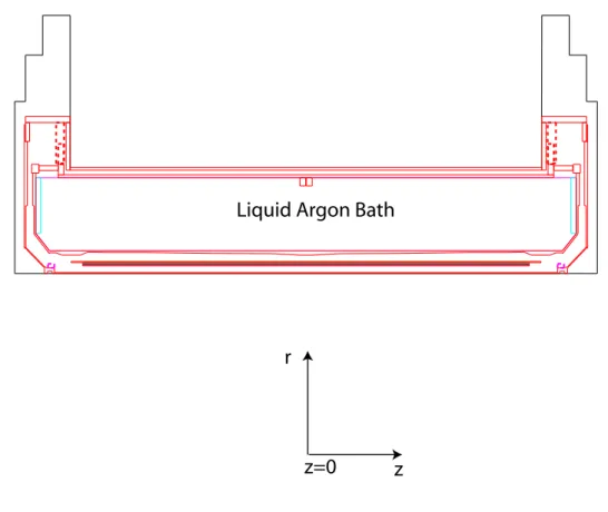
The GEANT description of the barrel cryostat is summarized in Fig. 7 and Fig. 8
Liquid Argon Bath
z r
z=0
FIG. 7: Description of the cryostat in the r-z plane (invariant under φ rotation). The red lines limit volumes in Al, the blue in Cu, the green in G10. Dashed lines show structures which cover only part inφ(see the following figure). The Al flange near z=0 and the volume for the LAr cable (in cyan) at high z are located within the main LAr bath volume.
In the central z part, the Al inner warm vessel of the cryostat starts atr=1150 mm and has a thickness of 10 mm . The coil starts at 1229 mm and ends at 1275.535 mm. It is composed of layers of Al (12.8, 13.8 and 12 mm thick), Cu (3.05 mm) and G10 (4.7 mm).
The Al inner cold vessel ends at r=1385 mm with a thickness varying withη (14 to 44 mm, see the figure). The outer Al cold vessel covers r=2140 to 2170 mm and the warm vessel 2220 to 2250 mm.
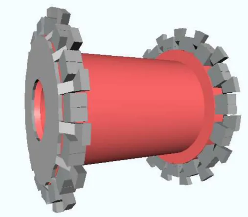
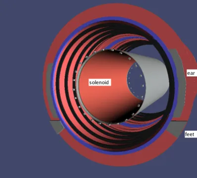
FIG. 8: A view of the cryostat in which several support structures are visible. Aluminum “feet”
welded to the warm vessel support the cold vessel via aluminum “ears”. The gap is filled, in reality, with G10. Small titanium blocks, mounted to a beveled surface (not shown) on the warm vessel, support the solenoid which lies in the vacuum between the warm and cold vessels via (unmodified) G10 triangular straps.
The ear and leg support at large z and large radius between the warm and cold vessels are shown in Fig. 8. They are made of Aluminum. The z thickness is 70 mm for the ear and 96 mm for the leg. The radial range is 2280-2490 mm for the ear and 2290-2710 mm for the leg. The upper and lower part of the ear are at y= ±1004 mm. The bottom of the leg is at φ=-37 deg. Support of the coil is provided by a series of titanium blocks welded onto the warm vessel, also visible in Fig. 8. Triangular supports made of G10 used to connect the coil to these blocks is presently not modeled in the simulation. A number of additional items are also not modeled, including:
• Additional Al plates (16 at each end, 25 mm thick) at highz and high radius between the cold and the warm vessels
• Feedthroughs/cables between the warm and cold vessel
• Some LAr bath at the high radius, high z part of the cryostat, near the feedthroughs More details on dead materials within the LAr system itself can be found in Section XI A.
Cables running from the inner detector to the electronics crates have a complicated com- position. Both the electronics crates and the cables from the inner detector are visible in Fig. 4. The description of these cables has required a intense effort, and is documented separately in reference [12].
C. Presampler geometry
The barrel presampler description in GEANT comes from D.Benchekroun, it was adapted to GeoModel by V.Tsulaia.
The LAr envelope in which the presampler is located starts at r=1410 mm and stops at r=1447 mm (the beginning of the LAr envelope of the accordion calorimeter). Each half- barrel presampler has 32 sectors in φ. Each sector is a LAr volume of thickness 29.98 mm in which the various presampler elements are located. The centers of the sectors are located on a circle of radius 1426 mm (see Fig. 9).
The transverse view of a sector is shown in Fig. 10. The width is 276.91 mm at the inner edge and 282.42 mm at the outer edge. The protection shell (thickness 0.4 mm), protection plate (thickness 0.5 mm) and the rails (thickness 8.58 mm, width 23.92 mm) are made of FR4 (mixture of hydrogen, carbon and oxygen, density 1.9 g/cm3, radiation length 211.08 mm). The motherboard (thickness 2.19 mm) is made of a mixture of FR4 and Copper (density 2.24 g/cm3, radiation length 127.19 mm). The cable thickness varies linearly with z from 1.5 mm to 5 mm with a width varying from 2.8 mm to 168.56 mm.
The cables are made of a mixture of copper, kapton, and liquid argon (density 3.98 g/cm3, radiation length 45.43 mm). The supports between the sector and the calorimeter inner G10 rings are ignored. Eight modules of differentz sizes are located in each PS sector (see Fig. 11).
Each module is a LAr volume in which the cathodes and anodes are located, as well as two prepreg plates (thickness 1 mm and 4.49 mm) made of FR4. The anode thickness is 0.329 mm and the cathode one is 0.2692 mm. They are made of a mixture of copper and FR4 (density 3.73 g/cm3, radiation length 46.3 mm for the cathode, density 3.06 g/cm3
FIG. 9: Position of the PS sectors inside the LAr envelope
Module Rail
Protection shell Protection plate
Connectic Rail Mother board
FIG. 10: Transverse view of one PS sector
radiation length 64.92 mm for the anode ). The “active” LAr thickness in a module is 13 mm (see section VIII for a more detailed discussion).
Table IV shows the z length of each module, the number of cathodes, the z separation between the cathodes (there is an anode in between two consecutive anodes), the angle of the electrodes, the number of readout cells (regrouping several gaps) and the z of the beginning of the first cell of the module. Fig. 12 and 13 show the third module in z as an
FIG. 11: Longitudinal view of one PS sector (note that the vertical sale is 18 times bigger than the horizontal one)
example. The beginning of the first module is at z=3 mm and the end of the last one at z=3082.13 mm.
TABLE IV: Parameters for the presampler modules
Module length (mm) N(catho.) ∆(z) catho. (mm) Angle (deg) N(cell) z first cell (mm)
1 285.67 56 4.974 25 8 3
2 294.99 64 4.609 12 8 288.67
3 320.28 72 4.448 0 8 583.65
4 355.89 80 4.448 0 8 903.93
5 403.76 88 4.588 0 8 1259.82
6 477.17 104 4.588 0 8 1663.58
7 561.75 128 4.387 0 8 2140.75
8 379.62 87 4.387 0 5 2702.5
D. Accordion calorimeter geometry
The calorimeter GEANT simulation was originally developed by G.Parrour and K.Kordas. The latest evolutions have been implemented by G.Unal
Electrode
FIG. 12: Transverse view of one PS module (the third in z)
FIG. 13: Longitudinal view of one PS module (the third in z)
The mother envelope of a half-barrel is shown in Fig. 14. It is filled with LAr. It goes from r=1447 mm (after the presampler) to r=2003.5 mm (end of the G10 outer bar). The inner z value of 3 mm is the beginning of the absorbers and electrodes. There is thus a gap of ± 3mm at z=0 between the absorbers of the two half-barrels. The non-projectivity of the end of the barrel near η 1.475 is taken into account in the simulation, see Fig. 15 for a view of the structure of the barrel near η 1.475.
r=1447 r=2003.5
z=3 z=3165
= 1.475 η
FIG. 14: Overall parameters of the calorimeter envelope
This mother volume is divided radially to create envelopes for the cables and mother- boards, the front G10 bar, the accordion structure and the back G10 bar. This division is shown in Fig. 16. The small straight sections at the beginning and the end of the ab- sorbers/electrodes are described in separate volumes as shown in the figure.
FIG. 15: View of the high-η part of the calorimeter
r=1447 14701490 1500.24
r=1970.48 1983.6 2003.5
G10 Bar
STAC volume: absorber and electrodes in LAr
Tip of absorbers and electrodes in LAr Cable and
motherboards in LAr
FIG. 16: Radial subdivision of the volumes in the calorimeter envelope
The description of the cables and motherboard follows the description written in[13]. An effective mixture for the summing board effect has been included. A zoom of the structure of this area for one module can be found in Fig. 17.
The thickness of the motherboard is 4.3 mm. It is described by a mixture of Cu and
Summing board effective Mixture
Cables
Motherboard
FIG. 17: Cable and motherboard structure for one module inφ
G10 given a density of 2.849 g/cm3 and a radiation length of 71.32 mm. The thickness of the cable varies linearly with z from 1 to 7.2 mm. The cables are described by a mixture
of Cu and Kapton given a density of 3.04 g/cm3 and a radiation length of 57.30 mm. The summing board+LAr is described by an effective mixture (thickness 10 mm) of Cu and Ar given density of 1.608 g/cm3 and a radiation length of 112.51 mm.
The G10 for the inner and outer bars has a density of 1.72 g/cm3 and a radiation length of 179.5 mm. The thickness is 20 mm.
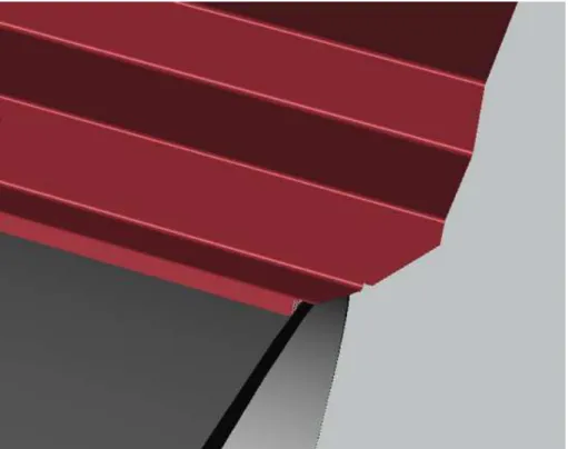
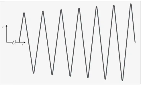
The accordion structure extends from r=1500.24 mm tor=1970.48 mm (starting at the first fold and ending at the last fold). It is a LAr bath in which the individual elements for the electrodes and the absorber are positioned. The electrodes and absorbers follow the same accordion shape (see Fig. 18 ), with different thicknesses (2.21 mm for the absorber and 0.275 mm for the electrodes). The absorber thickness corresponds to the average value given in the Barrel construction NIM paper[14]. The electrode is made of a mixture of Cu and Kapton, giving a density of 4.3236 g/cm3 and a radiation length of 34.744 mm. The absorbers are made of a mixture of lead, iron and glue[25]. For η less than 0.8, the mass fractions are 0.8254, 0.1517, and 0.0229, respectively, giving a density of 9.4749 g/cm3 and a radiation length of 7.4735 mm. Forη above 0.8, the mass fractions are 0.7466, 0.1859, and 0.0675 giving a density of 7.7326 g/cm3 and a radiation length of 9.7506 mm. In this case, the values for the thickness and the density are the values at warm. A contraction factor of 0.997 is used to obtain the cold characteristics (the thickness is reduced by this factor and the density is increased by the cube of this factor). Note that in the absorber structure a mixture is used and that the actual structures (lead and glue sandwiched between the steel skins) are not described in full detail. Even if the overall radiation length is the same, this could have a small effect on the signal visible in LAr (as the interaction of low energy electrons and photons depends on Z of the material). From a full simulation of a simple parallel-plate geometry, this seems to be a small effect. The free space between absorbers and electrodes is filled only with the LAr bath, and the effect of the honeycomb is neglected.
This will change by few % (volume effect) the signal in LAr, but should have a negligible effect on shower development and shower shape.
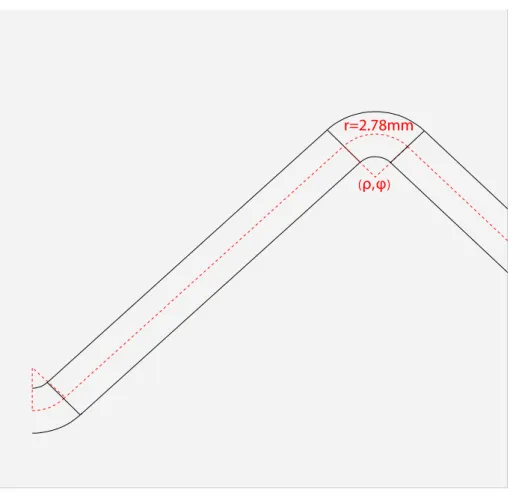
The absorber or electrode geometry is described in its internal frame, in which the x axis points along the axis of the absorber/electrode, oriented along the vector connecting the two endpoints of the accordion but originating near the origin of ATLAS coordinates.
In this frame, positions of the center of the circle corresponding to the folds are specified.
The radius of the fold (radius of the circle at the mid-line of the material) is 2.78 mm (see Fig. 19). The values (ρ,φ) in cylindrical coordinates of the center of the fold are summarized in table V.
TABLE V: Parameters for the accordion geometry. The φ values are computed in the internal frame, as defined in the text. The table applies to both electrodes and absorbers.
fold number ρ (mm) φ(deg) 0 1500.02 0.10619 1 1521.00 0.569751 2 1559.66 -0.573092 3 1597.20 0.576518 4 1634.57 -0.579943 5 1671.02 0.582296 6 1707.43 -0.585638 7 1743.07 0.588207 8 1778.67 -0.590596 9 1813.75 0.59285 10 1848.87 -0.595587 11 1883.36 0.59744 12 1918.02 -0.599714 13 1952.10 0.601911 14 1970.48 0.0811661
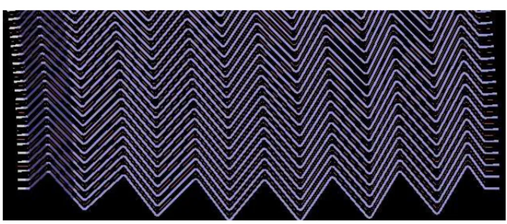
The 1024 absorbers and electrodes are positioned in the LAr by applying rotations in φ.
The small straight sections at the beginning (∆r=10 mm) and at the end (∆r=13 mm) of the accordion are described by placing small representative boxes in the LAr volume. For the front part, the Lead of the absorber is replaced by G10 for most of the radial space.
In this case, the detailed structure with the steel plate is described (as shown in Fig. 20), since the steel plate changes the average radiation length before the active volume by 2%X0 (45% X0 for 4.3% of the solid angle). Since this part of the structure is projective and the
x y
FIG. 18: Overview of non-sagging accordion structure. Note that the y scale is 10 times expanded compared to the x scale.
showers are very narrow at their beginning, this detailed description has been found to have a slight impact on the φ modulation of the energy response.
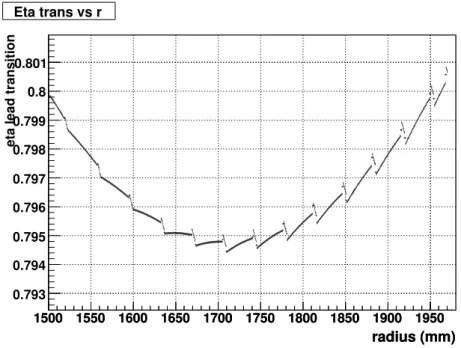
The transition at η=0.8 in the lead plates forms a straight projective line on the plate before folding. After folding, the transition on no longer at fixed η but varies with radius as shown in Fig. 21. This is accurately described in the geometry description.
In the simulation, the φ=0 axis of the nominal geometry is an electrode axis. The electrodes and absorbers run along the positive φ direction in the positive z barrel and, because of a relative rotation between the two barrels, in the negative φ direction in the negative-z barrel. The first absorber of the first cell is located before the first electrode, so its φ-position is at -2π/2048 for the positive-z barrel and +2π/2048 for the negative z barrel.
1. Sagging deformation
Sagging of the absorbers under the action of gravity is implemented in the accordion geometry (this is an option which is not active by default and is not turned on in the CSC production geometries). The mechanical sagging of absorber planes was computed recently at Orsay by A.Gallas with a finite element method. In this computation it is assumed
φ)
, ρ
(
r=2.78mm
FIG. 19: Detail of the accordion structure of one absorber. The electrode shape is the same with a different thickness.
that the inner radial and outer radial part of the absorbers remain in place and that the G10 rings stay perfectly circular. The sagging is described by a move in x-y local frame of each of the fold of the absorber (in the local frame, the x-axis is the absorber axis).
This computation was repeated for different orientations of the absorber. The maximal amplitude was normalized to the 1.2 mm displacement measured on a real absorber (the maximum sagging amplitude in the computation is 0.75 mm). The values of δx and δz for the folds of the absorber at φ=0 are given in the following table
G10 Absorber Steel (thickness=0.2 mm)
10 mm 2 mm
2.19 mm
FIG. 20: Detail of the description of the front tip of the absorber, between the inner G10 cylinder and the first accordion fold
radius (mm) 1500 1550 1600 1650 1700 1750 1800 1850 1900 1950
radius (mm) 1500 1550 1600 1650 1700 1750 1800 1850 1900 1950
eta lead transition
0.793 0.794 0.795 0.796 0.797 0.798 0.799 0.8 0.801
Eta trans vs r
FIG. 21: Transition between lead thicknesses in η (Atlas) as a function of radius, after folding of the absorber plate.
Fold δy (mm) δx (mm)
0 0 0
1 -0.064 0.032 2 -0.256 -0.128 3 -0.528 0.128
4 -0.8 -0.144
5 -1.008 0.144 6 -1.168 -0.064
7 -1.20 0
8 -1.152 0.064 9 -1.008 -0.112 10 -0.768 0.16 11 -0.512 -0.16 12 -0.256 0.176 13 -0.064 -0.064
14 -0 0