cognitive and decision-based model for pedestrian dynamics

cognitive and decision-based model for pedestrian dynamics

INAUGURAL-DISSERTATION

zur

Erlangung des Doktorgrades

der Mathematisch-Naturwissenschaftlichen Fakultät der Universität zu Köln

vorgelegt von

Cornelia von Krüchten

aus Köln

2019

Tag der mündlichen Prüfung: 29. Oktober 2019

Research on pedestrian dynamics is always an interplay between empirical and ex- perimental observations and theoretical modelling and simulations. Thereby, ped- estrian models are not only used for theoretically reproducing empirical data, but also to better analyse and understand the mechanisms and behavioural aspects that underlie pedestrian dynamics. The model approach that is presented in this work assumes pedestrian motion to result from cognitive and decision-based processes.

The model is set in continuous space, but discrete time and therefore belongs to a model class whose potential has been rarely investigated yet. However, com- pared to other model classes that are widely used in pedestrian dynamics, this approach is highly advantageous considering fidelity and simplicity in its structure.

A pedestrian is considered as an autonomous entity that gains information on the surrounding by visual perception and anticipation. On this basis, the agent takes a decision on its movement for the next time step.

The main focus during the development of the approach was on modelling the in- teraction and collision avoidance with other agents. Particularly for the collision avoidance, stochastic procedures are used in order to consider uncertainties of hu- man decisions explicitly which makes the modelling approach more realistic.

As simulation results show, the new approach is able to reproduce characteristic effects of pedestrian motion very well. For typical scenarios that have been used as test cases the simulated results fit well, at least qualitatively but often even

by modelling individual interaction of a single pedestrian with others. During the development of the model its parameters were specifically adjusted for the single scenarios, considering the empirical data basis. In addition, several cognitive mech- anisms were supplemented. By this means, it is possible to identify and understand the important intrinsic properties and motivations of a pedestrian. Furthermore, this provides the opportunity to gain insight into how cognitive and decision-based approaches can model pedestrian behaviour as realistically as possible.

Die Erforschung von Fußgängerdynamik ist stets ein Zusammenspiel aus empi- rischen und experimentellen Beobachtungen und theoretischer Modellierung und Simulationen. Dabei sind Modelle nicht nur eine theoretische Reproduktion em- pirischer Daten, sondern eine wichtige Informationsquelle, um die Mechanismen und Verhaltensweisen, die der Fußgängerdynamik zugrunde liegen, zu analysieren und zu verstehen. In dieser Arbeit wird ein neuer Modellansatz vorgestellt, der die Bewegungen von Fußgängern als Resultat kognitiver und entscheidungsbasierter Prozesse auffasst.

Das Modell ist raumkontinuierlich, aber zeitdiskret und gehört damit zu einer Mo- dellklasse, deren Potential bisher wenig untersucht wurde, die aber im Vergleich mit den üblicherweise verwendeten Klassen große Vorteile in Bezug auf Genauigkeit und strukturelle Einfachheit hat. Ein Fußgänger wird als eine autonome Einheit betrach- tet, die mittels visueller Wahrnehmung und Antizipation Informationen über ihre unmittelbare Umgebung sammelt, und auf dieser Grundlage über ihre Bewegung im nächsten Zeitschritt entscheidet.

Ein Hauptaugenmerk in der Modellentwicklung lag auf der Modellierung der Inter- aktion und Kollisionsvermeidung mit anderen Agenten. Unter anderem an dieser Stelle wird insbesondere auf stochastische Prozeduren zurückgegriffen, die die Unsi- cherheiten und Unwägbarkeiten menschlicher Entscheidungen berücksichtigen und dabei helfen, den Modellansatz realistischer zu machen.

quantitativ sehr gut zu modellieren. Im Besonderen können wichtige makrosko- pische Effekte, speziell kollektive Phänomene, durch die Modellierung von indivi- dueller Wechselwirkung eines Einzelnen mit anderen Fußgängern gut reproduziert werden. Während der Modellentwicklung wurden die verwendeten Parameter im Hinblick auf die empirische Datengrundlage situationsspezifisch angepasst und wei- tere kognitive Prozeduren ergänzt. Damit können zum einen die ausschlaggeben- den intrinsischen Eigenschaften und Motive eines Fußgängers besser identifiziert und verstanden werden, zum anderen Erkenntnisse darüber gewonnen werden, wie kognitive und entscheidungsbasierte Modelle realistisches Verhalten für Fußgänger bestmöglich wiedergeben können.

Abstract i

Kurzzusammenfassung iii

1 Introduction 1

2 Pedestrian Dynamics 3

2.1 Empirical and Experimental Observations . . . . 3

2.2 Modelling Pedestrian Dynamics . . . . 10

2.3 Concepts Included in the Model . . . . 18

3 The Model 25 3.1 Concept, Classification and Structure . . . . 25

3.1.1 Concept of the Model . . . . 26

3.1.2 Classification of the Model . . . . 27

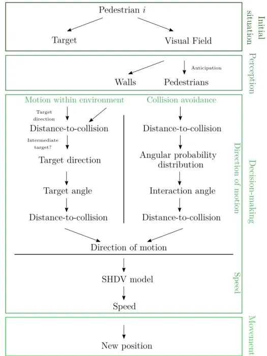
3.1.3 The Structure . . . . 27

3.2 The Model Components . . . . 30

3.2.1 The Environment . . . . 30

3.2.2 The Agent . . . . 31

3.3 The Perception Phase . . . . 32

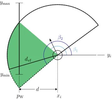
3.3.1 Perception of Walls . . . . 33

3.3.2 Perception of Pedestrians . . . . 34

3.4 The Decision Phase . . . . 37

3.4.1 Motion within the Environment: Decision on Target Angle . 38 3.4.2 Collision Avoidance: Interaction Angle . . . . 41

3.4.3 Choice of the Direction of Motion . . . . 43

3.4.4 Determination of Speed . . . . 44

3.5 The Movement Phase . . . . 44

4 Modelling Results 47 4.1 Collision Avoidance Behaviour . . . . 47

4.2 Single-File Motion . . . . 56

4.2.1 Fundamental Diagram . . . . 57

4.2.2 Phase Separation . . . . 68

4.3 Evacuation . . . . 71

4.4 Bidirectional Flow . . . . 85

4.5 Summary . . . 100

5 Conclusion and Outlook 101 Bibliography 105 A Parameters of the model 125 B Determination of Angles and Distances 129 B.1 Determination of Angles . . . 129

B.1.1 Viewing Angle in Wall Perception . . . 129

B.1.2 Angle Between x-axis and the Connecting Line Between Ar- bitrary Points in Space . . . 133

B.1.3 Transformation from Absolute to Relative Perception Angle 135 B.1.4 Angular Extension During Perception of Pedestrians . . . . 138

B.2 Distance-to-Collision . . . 140

B.2.1 Distance-to-Collision to Walls . . . 141

B.2.2 Distance-to-Collision to Pedestrians . . . 148

B.3 Probability Distribution for Collision Avoidance and Interaction Angle150 B.3.1 General Approach . . . 151 B.3.2 Calculation of the Normalisation Constant . . . 153 B.3.3 Calculation of the Interaction Angle . . . 162

C Determination of Density and Velocity 167

C.1 Global Fundamental Diagram . . . 168 C.2 Local Fundamental Diagram . . . 170

D Evacuation 171

Danksagung 177

Erklärung 179

CHAPTER 1

Introduction

‘Pedestrian dynamics’: basically everybody has at least a general idea what is meant by this expression. On the one hand, walking is the most natural form of human locomotion and a vast majority of us is part of road traffic as a pedestrian routinely. On the other hand, crowd disasters are also part of the public awareness.

Research on pedestrian dynamics therefore often focuses not on the investigation of the motion of single individuals, but pedestrians in large groups and their inter- action with others and the environment.

But, is this physics? In physical systems, particles are often considered as passive entities, exposed to extrinsic impacts, described by observables. In contrast, a ped- estrian his- / herself would probably claim decision-making independence for his / her walking behaviour. Large pedestrian groups, especially in the light of crowd disasters, are often publicly referred to as ‘panicking’ masses showing irrational and asocial behaviour (see Sec. 2.1). In fact, it is often claimed that including behavi- oural aspects in pedestrian models makes them realistic [1–5].

Physics-based models are nevertheless able to reproduce pedestrian motion realist- ically for different situations. From a physicist’s point of view, a pedestrian crowd can be considered as interacting particles that can be described e.g. in analogy to classical fluid or gas mechanics [6–8]. Other approaches use statistical phys-

ics to represent crowds as many-body systems in non-equilibrium states exposed to stochastic processes [9–11]. Pedestrians can be regarded as driven by external forces similar to Newtonian mechanics [12] or by minimising potentials [13]. An important characteristic feature of crowds is the emergence of self-ordering or col- lective phenomena. Due to microscopic interactions, the system spontaneously shows macroscopic effects, like stop-and-go waves or lane formation in counterflow.

Some of these phenomena are also observed in totally different systems: intermit- tent egress flows at bottlenecks were observed for pedestrians, sheep or granular material [14, 15]. Lane formation could also be found for self-driven particles and colloids, see e.g. [16–18]. In a simple model for self-driven particles, Vicsek et al. found cooperative motion and self-ordering [19]. They predicted a continuous phase transition from a homogeneous to an ordered state, which is also assumed in models for pedestrian lane formation [9, 20]. Since these systems involve particles that are not naturally assigned with psychological mechanisms, it is still reasonable to describe pedestrians (also) as a physical system, especially at high densities. It might be necessary to combine both aspects, physics and psychology, in order to yield an understanding of the underlying principles of pedestrian motion.

In this thesis, a new modelling approach for pedestrian dynamics is presented that is physics-based and captures a pedestrian as an actively deciding agent. It tries to gain insight into coherencies of pedestrian motion by reproducing realistic dy- namics. A pedestrian’s decision on its velocity, both direction and absolute value, is modelled using a simply structured set of rules. An agent has cognitive abil- ities like perception or decision-making which are used to navigate through the surrounding infrastructure and to respond to other pedestrians. The approach belongs to a model class that combines aspects of different approaches and that has been sparsely investigated yet. It shows realistic behaviour that fits well to empirical data for collision avoidance, single-file motion, evacuation scenarios and bidirectional flow. It reproduces collective phenomena like stop-and-go waves, lane formation or clogging at bottlenecks. During the optimisation process, the model provides insight into a pedestrian’s intrinsic prioritisation and decision behaviour.

CHAPTER 2

Pedestrian Dynamics

A pedestrian is ‘a person moving on foot in a publicly accessible area’ [21]. As simple as this seems to be, research on pedestrian dynamics comprises not only many different approaches, methods and models, but is also influenced by a wide variety of research fields like physics, psychology, sociology, mathematics, engineering or computer game development. Each of these can only consider certain aspects of all coherences that influence pedestrian walking behaviour (yet). In this chapter, a short overview over central aspects of pedestrian dynamics is given, followed by a more detailed description of mechanisms with particular importance for the new model approach presented in this thesis. If not stated otherwise, the overview is based mainly on [22–24].

2.1 Empirical and Experimental Observations

Much insight into pedestrian dynamics is gained by either controlled experiments or empirical observations. Beneath qualitative results, pedestrian walking behaviour can be described quantitatively. In this context, three quantities are of major importance: the pedestrian density ρ, velocity v and flow J. There are multiple

approaches how to define and measure pedestrian density and velocity which are more or less suitable for different scenarios. The pedestrian flow is given by the number of agents passing a fixed measurement area of width b [21, 24],

J =ρvb [1/time], (2.1)

and is usually considered as a scalar quantity since the normal component of the velocity with respect to the measurement line is used. The hydrodynamic re- lation describes the specific pedestrian flow as the number of pedestrians passing the measurement area per unit time and width:

J_s =ρv [1/(width·time)]. (2.2)

The correlation between these three basic quantities is expressed via the fun- damental diagram. It describes the relationship between flow or velocity and density and is, as its name implies, one of the most important observables in pedes- trian dynamics. In modelling, it is often used for calibration or validation purposes or as input parameter [25]. Measured fundamental diagrams in part differ signific- antly [26], in addition their shape can depend on the specific scenario [21, 25, 26]

or the measurement method [25, 27, 28]. However, all diagrams consistently show a decrease in the velocity for an increasing pedestrian density [26].

In general, the capacity of a system is given by the maximum number of pedes- trians which is able to sustain a certain action (e.g. walking, standing, crossing) within the facility [21]. In fundamental diagrams, the capacity is given by the max- imum flow, and the corresponding system state is referred to as ‘capacity state’, the respective density as ‘critical density’¹. For density values below the critical density, the system is in the free-flow phase, where the pedestrians can move with their preferred velocities without congestion; for densities above the critical density, the system is in the congested state and the flow decreases with increasing density [29].

1In this case ‘critical’ does not necessarily refer to criticality in the physical sense.

One of the most interesting characteristics of pedestrian dynamics is the emergence of collective phenomena or behaviours which is also referred to as ‘self-organisation’

[25, 29, 30]. These phenomena are macroscopically observable behaviours caused by individual, microscopic dynamics. As distinguished from aggregate behaviour, col- lective motion arises from spatial or temporal synchronisation of the crowd members [21]. There are several typical collective behaviours that are repeatedly observed for walking pedestrians.

Jamming, Clogging and Arching

Jamming and clogging are phenomena observed at high densities. Jamming usually occurs if the inflow or the number of pedestrians in a system exceeds the system’s capacity, for example at narrowings or in counterflow scenarios, such a scenario is shown in Fig. 2.1(a) for an evacuation through a narrow door. Clogging can occur in pedestrian groups with a high urge to enter a facility of limited capacity, e.g.

exits. The pedestrians form short-lived structures around the exit which often have a semi-circular shape. Due to these arches the participants block each other and the flow is decreased or interrupted [21–24].

Bottleneck Flow and Evacuations

Bottlenecks, in general, are spatial structures with limited capacity, e.g. the door in an evacuation scenario or a narrowing in a corridor [22]. For high densities, they can cause the reduction of flow and emergence of jamming [21]. In bidirectional motion, oscillations of the direction of motion through a narrow bottleneck occur. To reduce the number of interactions, several pedestrians of the same direction of motion pass the bottleneck consecutively before the situation changes and a person with opposite direction is able to pass. This person is again followed by other pedestrians with the same direction so that the direction of motion within the bottleneck changes in an oscillatory way [22, 24, 25]. At narrowings in corridors several collective phenomena can be observed. If the inflow is large enough, jamming occurs and the pedestrians wait in a cluster in front of the bottleneck [33] (see Fig. 2.1(a)).

(a) Jamming in front of an exit (screenshot from [31])

(b) Scheme of the zipper effect in corridors (from [32])

Figure 2.1: (a) Jamming in an evacuation scenario, the pedestrians wait in a dense group in front of the exit. (b) With an increasing width of a corridor the pedestrians increasingly walk in a zipper-like configuration and the flow increases approximately linearly.

Thereby, the density within the cluster usually does not depend on the width of the bottleneck, but decreases significantly within it [34]. The flow within the narrowing depends on its width. With increasing corridor width the pedestrians use the available space most efficiently by decreasing the interpersonal distance along the direction of motion while increasing the lateral distance. This behaviour is called ‘zipper effect’ (see Fig. 2.1(b)). It causes an almost linear increase of the maximum flow within the bottleneck with increasing corridor width [27]. At sufficiently high densities and desired velocities, clogging is observed at bottlenecks.

The blockages lead to intermittent flows which show large time gaps between single pedestrians alternating with larger groups of pedestrians passing in a short space of time, so-called ‘bursts’ [15, 35, 36]. This is particularly important for evacuation scenarios in which the exit acts as a bottleneck for the egressing pedestrians. Muir et al. [37] showed for evacuations in airplanes that competitive behaviour can cause blockages of the exit and increase the egress times. The negative impact of

competitive behaviour on the total evacuation time is sometimes also referred to as

‘faster-is-slower’ effect [38]. Here, the competitiveness and higher urge to leave the room is interpreted as a higher desired velocity of the pedestrians (‘faster’) that causes increased evacuation times (‘is slower’).

Lane Formation

Lane formation in general describes the emergence of elongated clusters (‘lanes’) of pedestrians with the same walking direction along the direction of motion [21]. This self-ordering is often observed in bidirectional flow [25, 39–41] as shown in Fig. 2.2.

By following other pedestrians with the same direction of motion, the number of interactions and collisions with oppositely walking agents is reduced [41]. This enhances comfort and smooth motion [25, 30]. As a result, the pedestrian flow is stabilised compared to the unordered system and the velocity of the agents increases [39, 40]. Lanes in bidirectional motion can be either stable, separating the system into, mostly two, regimes of opposite walking directions, or so-called dynamic multi- lanes [41]. Dynamic lanes can arise, decay or merge with other lanes, so that the number of lanes in the system varies in time. Lane formation requires a sufficiently high density and may depend on external components like boundary conditions or additional instructions, e.g. which side should be preferably chosen when evading an oppositely walking pedestrian [29].

Patterns in Intersecting Streams

At crossings and intersections, pedestrians show routes deviating from the supposed optimal or shortest route, e.g. short-lived roundabouts [22–24] or diagonal stripe formations [43]. They enhance the efficiency of the walking behaviour.

Density and Stop-and-Go Waves

Density waves are quasi-periodic changes of the density in space and time that are mostly observed in high-density scenarios. A typical example in pedestrian dynam-

Figure 2.2: Lane formation in bidirectional flow in a corridor. Pedestrians with black shirts are walking from left to right, participants with red shirts from right to left (screenshot from [42]).

ics are stop-and-go waves similar to those of vehicular traffic [22–24]. They can be observed in both empirical observations [44] and controlled experiments. Stop- and-go waves in pedestrian dynamics occur especially in one-dimensional single-file motion [27, 45–49]. Above a certain critical density, the formation of jams can be observed that separate the system into standing and moving pedestrians, whereby the density within the jams is increased compared to the rest of the system. This fluctuation in the density propagates in the opposite direction than the walking dir- ection of the pedestrians. In vehicular traffic, the system separates into a jammed phase with standing cars and a free-flow phase with fast moving vehicles [23, 50]. In contrast, stop-and-go waves in pedestrian dynamics show separation into a standing and a slowly moving phase.

Collision Avoidance

Collision avoidance with static and moving obstacles is one of the basic interac- tion mechanisms of pedestrians and can, for example, be particularly observed at

intersections. It comprises adjustments of the walking speed and the direction of motion. Whether an agent slows down or evades the collision, can depend on mul- tiple factors.

In laboratory experiments on crossing scenarios of two pedestrians (approaching each other at an angle of 90^◦), most collisions (∼94%) are avoided because at least one of the agents changes its velocity [51]. In the majority of cases (∼ 65%), one of the agents increases its speed, whereas the other one slows down. In other cases, both pedestrians either increase or decrease their speeds, or only one of the agents accelerates, whereas the opponent keeps its velocity. In contrast, Parisi et al. [52]

observed that at crossings at 90^◦ and 180^◦ collisions in low-density situations were mainly avoided by adjusting the direction of motion. For higher densities, steering in encounters with 180^◦ was less often and less distinct compared to crossings at 90^◦. Overall, the authors found that pedestrians are three times more likely to change their direction of motion than stop. Similar to that, the experimental res- ults from Huber et al. [53] showed that adjustments of the speed were only used if the angle with the groups of participants and a crossing interferer was 45^◦ or 90^◦, whereas changes in the walking directions were also observed for 130^◦ and 180^◦. It is assumed that collision avoidance by adjusting the speed is used if the available space or time is restricted, while evading manoeuvres are applied more generally.

Psychology in Pedestrian Dynamics

In contrast to passive, non-autonomous particles, pedestrians can be considered as intelligent humans with a certain awareness about themselves. In terms of physics, a ‘crowd’ is mostly understood as a group of people who are on the same place at the same time. However, in the framework of the social identity theory a ‘physical’

crowd can involve one or more ‘psychological’ crowds [21]. Pedestrians within a psychological crowd understand themselves as part of a group and can distinguish between group members and others, while physical crowds describe pure aggreg- ations of people. This self-categorisation can have an influence on the behaviour and interaction of the pedestrians [2–4].

There are several contributions which recommend the explicit incorporation of so- cial and psychological aspects in pedestrian models in order to describe walking behaviour realistically [1, 3, 5, 54]. However, reliable experimental or empirical data are rare. Von Sivers et al. [2, 3] implemented previously observed social identity and helping behaviour in an terroristic incident which affected the overall evacuation time. In evacuation experiments, Garcimartin et al. [38] observed a negative influence of competitive behaviour on egress times, while Muir et al. [37]

observed that competitiveness was disadvantageous in terms of evacuation times for small bottlenecks, but decreased the egress times for larger widths. Sieben et al. [5] aimed at capturing the influence of social norms and social psychology on the waiting behaviour of pedestrians in front of bottlenecks.

The public perception of pedestrian dynamics is probably highly connected to ideas of ‘panic’ or ‘mass panic’. Thereby, one should consider that there is no consensus on the definition of the term ‘panic’. In most cases it is understood as an irrational, asocial response to a potential threat or danger [55, 56]. However, panic in this view does not occur as often in pedestrian crowd incidents as assumed [55]. In fact, it has been observed that in states of fear, humans rather look for familiar persons and places than flee blindly [56, 57]. Showing this ‘affiliate behaviour’ [56], help and cooperation dominate in critical situations (see also [2, 3] and references therein).

2.2 Modelling Pedestrian Dynamics

As experiments and empirical studies on pedestrian dynamics are often difficult and for some situations even not possible for practical, ethical or financial reasons, simulation and modelling of pedestrian walking are two very important aspects of this research field. Over the years, lots of different model approaches have been developed and improved. Only in a recently developed glossary for pedestrian dy- namics [21], 17 different sub-categories for pedestrian models were found. Therefore, the overview given in this section only describes a small subset in greater detail.

Classification of Pedestrian Models

Based on the modelled time scale, pedestrian models can focus on different levels of walking behaviours [22, 24, 58]. On a strategic level, a pedestrian decides on actions in the longer run, considering the superordinate goal. In contrast, decisions on the tactical level are on short-term planning of the actions based on the current situations and comprises for example route choice behaviours. On the third, operational level, the actual walking dynamics is determined. These level dis- tinguish themselves also by the degree of cognition and autonomy of the agents:

whereas operational level models are often physics-based approaches and can rep- resent pedestrians as simple particles, decisions on the tactical and strategical level require higher cognitive abilities and are therefore related to psychological and so- ciological effects. Models dealing with ‘intelligence’ often combine operational with tactical or even strategical decisions.

The majority of pedestrian models consider the operational level which is mainly de- termined by physics. They can be further classified based on the agents’ autonomy [25] or underlying structure [22, 24] as described in the following.

Relying to the simulated length scale, pedestrian models can be macro-, meso- or microscopic. Macroscopic models describe the state of the system by global, averaged quantities like density or flow using conservation laws or continuity equa- tions. Individual agents are indistinguishable [59]. Typical examples for macro- scopic models are fluid or gas-kinetic models that treat the crowd of pedestrians analogously to a gas or fluid [6, 7, 60–63]. The crowd is considered as a continuum [8, 64, 65]. Models on a mesoscopic scale consider the agents as individuals, but describe the system globally by probability distributions [21]. They are often also referred to as ‘kinetic models’ and can be used as intermediate step when deriv- ing a macro- from a microscopic model [8, 43, 65, 66]. In microscopic models, pedestrians are described as distinguishable particles or agents whose state is char- acterised by microscopic variables like velocity or position. They can be further categorised [22, 24]: microscopic models can be heuristic, if the dynamics is mainly determined by pedestrian interaction, or first-principle models where

the dynamics is characterised by pre-defined principles. With respect to the nature of the variables used in the models, they can either be discrete orcontinuous, depending on whether the values of the parameters are integers or arbitrary real numbers, respectively. In general, each combination of discrete and continuous quantities is possible. Moreover, model approaches can use stochastic elements which add uncertainties to the system. Whether it is used as probabilities for decision-making processes or as noise signals added to the system, the stochasticity can be regarded as ‘intrinsic’ or ‘extrinsic’. In contrast, in deterministicmodels the system state at a future time is fully pre-determined by the present state. With same initial conditions the time evolution of a deterministically modelled system will always be the same. These models neglect a lack of knowledge of underlying mechanisms in pedestrian dynamics which make the motion more unpredictable.

Therefore, they are often regarded as less realistic than stochastic models.

Based on how the dynamics of the model is formulated, microscopic models can be categorised as acceleration-, velocity- or decision-based. Acceleration-based, also called force-based or second-order models, use analogies to Newtonian mechan- ics to describe the movement of the particles as determined by forces. In contrast, in velocity-based models, the pedestrian’s velocity (absolute value and direction) is directly determined based on the current state of the agents and the environ- ment. They often use visual perception of the pedestrians to gain the information and rely on optimisation problems for interaction. Rule-based models are also called ‘position-based’ as they do not use any velocity- or acceleration-based for- mulation. In fact, the state of a pedestrian is determined by decisions which are modelled using a fixed set of rules. Two commonly used model classes are described hereinafter.

Social Force Models

In force- or acceleration-based models, the pedestrian is exposed to external and internal forces that determine its dynamics. In doing so, they rely on an analogy to Newtonian mechanics. These models are often fully continuous and deterministic

[67–69]. One of the most known acceleration-based models is the Social Force Model by Helbing and Molnár [12]. The dynamics of a pedestrian i is given by the equation of motion,

dvvv_i(t)

dt =FFF_i(t) =FFF^(driv)_i +FFF^(soc)_i +FFF^(phys)_i . (2.3) Here, the forces acting on the pedestrian can be summarised as the driving force FFF^(driv)_i , social forces FFF^(soc)_i and physical forces FFF^(phys)_i . The driving force displays the pedestrian’s aim to move with its desired velocityvvv^(des)_i and to reach it within the relaxation time τ_i:

FFF^(driv)_i =vvv^(des)_i −vvv_i

τ_i (2.4)

The social force FFF^(soc)_i is the sum of all forces ‘felt’ by the agents exerted by oth- ers or elements of the environment like walls or obstacles. In terms of personal space and safety distance, social forces are usually repulsive, but can also include attractive components than depend on the relative distance or are used to model group cohesion [22, 24]. In centrifugal force models [70, 71], the repulsive force by other pedestrians additionally depends on the relative velocities of two interacting agents. Physical forcesFFF^(phys)_i are included for physical interactions like collisions, e.g. to prevent excessive overlapping.

Although social force models are commonly used for pedestrian dynamics, they show two inherent problems, first, with the underlying mechanical approach, second with the numerical calculation of the equation of motion.

While being related to Newtonian mechanics, social forces do not obey Newton’s Third Law ‘actio = reactio’ [72, 73]. For example, an agent could exert a social force to another pedestrian which does not lie within the agent’s vision and there- fore cannot exert an opposite force of the same magnitude. In addition, the total force acting on a pedestrian is given by the superposition of driving, social and physical forces, see Eq. (2.3). Especially at high densities or for an increasing range of the forces, this can lead to unwanted backwards motion or unrealistically high velocities which exceed the desired speed [72, 73], or the occurrence of collisions

instead of stable jam formation [74]. Another characteristic for systems in Newto- nian mechanics is the usage of inertia which is modelled as the mass of a pedestrian in force-based models (in Eq. (2.3), the mass m_i is not neglected, but set to 1). It is indicated, however, that inertia only plays a minor role in pedestrian dynamics since pedestrians are able to stop and accelerate almost immediately [75]. Inertia related ‘overreactions’ of the pedestrians lead to oscillations in the movement and collisions with others [73].

Köster et al. [76, 77] give a detailed description of the numerical problems of the social force model when solving the equation of motion which are mainly caused by discontinuities of the forces in Eq. (2.3). For example, the driving force FFF^(driv)_i is determined by the preferred velocityvvv^(des)_i which always points towards the agent’s target,

vvv^(des)_i =v⁰_i rrr_tar−rrr_i

|rrr_tar−rrr_i| (2.5)

with the position of the target rrr_tar, the current position of pedestrian i, rrr_i, and the desired absolute value of the speed, v_i⁰. As can be seen from Eq. (2.5), the driving force has a singularity at the target position. When solving the equation of motion computationally, numerical schemes as the commonly used Euler scheme lose their accuracy and cannot converge. In order to solve the equation of motion, it is rewritten as difference equation discretising the time. This difference equations, however, result in oscillating solutions for trajectories in the vicinity of the target.

Therefore the agent is not able to approach its goal but stays on a stable orbit around it with a constant speed. Decreasing the time step weakens this effect, but increases the computation time. Therefore, discontinuities in the equation of motion must be approached explicitly by mollification in order to obtain realistic results [76, 77].

Cellular Automaton Floor Field Models

Whereas social force models are mostly fully continuous, acceleration-based and deterministic, cellular automaton (CA) approaches are categorised on the other side

of the spectrum as fully discrete, stochastic and rule-based models. In CA models, time, space and state variables like the velocity are discrete [10, 11, 78]. The two- dimensional space is divided into, mostly square cells, whose size represents the space requirement of a pedestrian in a dense crowd, approximately 0.4 m×0.4 m [26]. The dynamics is performed in discrete time steps whose size is often associated with a pedestrian’s reaction time between 0.1− 0.3 s. If a particle can move in every time step, ∆t = 0.3 s leads for this cell size to a velocity of 1.3 m/s which is consistent with a pedestrian’s free flow speed [10]. Pedestrians are represented as particles which obey the exclusion principle: a cell can only be occupied by one particle at the same time. The dynamics is determined by probabilities for the transition of a particle towards a cell within its neighbourhood. In most cases, the velocity of the particles is restricted to one cell per time step. Usually, two different neighbourhood concepts are used: the von Neumann neighbourhood comprises the four cells to the front, back, left and right, whereas the Moore neighbourhood additionally includes the diagonal cells.

After few simple approaches to apply CA models on pedestrian dynamics, e.g.

[9, 79], Burstedde et al. [11] proposed an extended version of a CA model which is now commonly used in pedestrian research, the Floor Field Model.

In order to approach the long-ranged interactions between pedestrians, the authors resort to a concept of chemotaxis as observed e.g. for ants. By means of floor fields, these long-ranged interactions can be transformed to short-ranged, local ones, which decreases the computational effort significantly. A pedestrian that moves away from a specific cell (i, j) leaves some kind of ‘markers’ which can be felt and traced by other agents. The information on these markers is stored in the so-calleddynamic floor field D_ij. The dynamic floor field is influenced by the pedestrians and determines the transition probabilities of the cells. It can be understood as a virtual trace left by the agents. Additional to the influence of the particles, the dynamic floor field changes in time by decay and diffusion and therefore has its own dynamics. Besides the interaction with other pedestrians, the agent tries to walk into its preferred direction. This information is provided by the matrix of

preference which gives the transition probabilities for the neighbouring cells of an agent considering e.g. the desired direction or the average velocity of the system.

Thereby, each particle has its own 3×3 matrix of preference for each time step. This approach can be improved when considering an additional floor field, the static floor field S_ij, which represents information on the environment and preferred direction [10]. It is usually equal for all agents and constant in time and gives the shortest way from the cell to the destination. Using this floor field, the matrix of preference can be omitted. Considering both floor fields, the final transition probability p_ij for a cell (i, j) is given by

pij =Nexp (k_SSij) exp (k_DDij) (1−nij)ζij. (2.6) N is the normalisation constant, S_ij and D_ij the values for the static and dynamic floor field, respectively, which are considered for the probability by a respective coupling constant kS and kD. The obstacle number ζij is zero for cells that are forbidden due to the environmental components like walls, and otherwise equal to one. The occupation number is n_ij = 1 for occupied cells, and n_ij = 0 for empty ones.

Based on the discrete time, the system update is usually performed in parallel. In this case, conflicts can occur whenever two or more particles have the same target cell. They can be solved in each time step [11] or approached more complexly using a friction parameterµwhich gives the probability that none of the particles is allowed to move to the target cell and the conflict remains unsolved [80]. Accordingly, with probability 1−µ one of the agents is chosen randomly and moves to the target.

It can be shown that friction helps at the description of clogging at bottlenecks.

Beneath a single parameter, also friction functions can be used which also consider the number of particles involved in the conflict [81].

The spatial discretisation of CA models leads to some internal problems. More complex geometries with structures incommensurate with the size of a cell may not be representable in full detail, and microscopic assessment of trajectories or other locally measured quantities is not easily possible [10]. When using a Moore

neighbourhood, where diagonal motion is allowed, the total distance covered in one time step can be higher compared to straight motion to the front / back or to the left / right [82–84]. Therefore, the effective velocities vary depending on the chosen direction. This can be diminished when using the matrix of preference or smaller cells. Smaller cells, however, lead to new problems considering the resolution of conflicts.

Application of Models

In general, reproducing collective phenomena in pedestrian motion is a commonly used way to assess the performance of a model. Over the years, different types of collective motion were observed in simulated results. Pedestrian models are able to reproduce oscillatory changes of the direction of motion at bottlenecks [85–87]

as well as intermittent flows in evacuation and bottleneck scenarios by clogs and bursts [15, 35, 88–92]. Also the empirically observed detours at intersections and crossings are found in simulation results [8, 43, 87].

The fundamental diagram is one of the most essential quantities in pedestrian mo- tion and often used for calibration purposes [78]. However, it is a non-trivial prob- lem to obtain realistic fundamental diagrams in pedestrian models. For example, the original social force model [12] seems not to be able to reproduce a fundamental diagram either in unidirectional flow in a corridor [93], or in one-dimensional single- file motion [94, 95]. Realistic results are only obtained with additional concepts and adjustments [93, 96]. Even for a simple CA floor field model, a good fit of the fun- damental diagram to experimental data requires velocities larger than one cell per time step or an additional ‘politeness factor’ [78]. How well it fits often also de- pends on the measurement method [13, 78]. Velocity-based and heuristic models can reproduce fundamental diagrams mainly qualitatively [97–102].

Stop-and-go waves, especially for one-dimensional motion can also not be simulated by classical social force models [103, 104]. They were observed only in models that explicitly adjust the agent’s velocity [45, 47, 102] or that add additional noise or small inhomogeneities to the modelled system [105, 106].

When simulating bidirectional flow in corridors, several model approaches repro- duce stable lanes that cause a separation of the system or dynamically varying lanes. In either case, the walking behaviour of the agents is improved [107–112].

However, many model approaches have to cope with total blockages of the corridor, also referred to as ‘gridlock’, ‘jamming’ or ‘freezing’ state, these states are usually very stable and persist until the end of the simulation [9, 11, 29, 112–118]. As no such behaviour is found in reality, it must be an artefact of the model approaches.

2.3 Concepts Included in the Model

Social force models and CA floor field models are ‘extremal examples’ of model classes. Both approaches have advantages and drawbacks, which can significantly influence the simulation results. Therefore, the model presented in this work aims at a hybrid approach which includes aspects from several model classes in order to obtain optimal results. Characteristic features of this approach are:

• Continuous space and discrete time: there are no spatial artefacts as in CA ap- proaches and no numerical artefacts as in force-based models. The approach uses the time-discrete and space-continuous Stochastic Headway Dependent Velocity model [102, 119, 120] as a basis.

• Introduction of cognitive abilities: the pedestrian has visual perception, an- ticipation, decision-making and navigation.

• Velocity adaptation based on the perceived environment: the agent decides actively on its speed by recognising and assessing the current situation. The concept of a ‘distance-to-collision’ is used as basis of decision-making.

• Stochasticity instead of optimisation problems: the pedestrians are not as- sumed to decide optimally for every time step, the behaviour is more uncer- tain.

Many of these concepts are also applied in different models. They mostly consider cognitive or perceptual abilities of the agents.

The SHDV Model

The Stochastic Headway Dependent Velocity (SHDV) model was developed in 2014 by C. Eilhardt and A. Schadschneider and acts as a basis for this new approach.

Extended into two dimensions in this thesis, the SHDV model was originally de- veloped in order to reproduce and analyse phase separation at high densities in pedestrian single-file motion. The following description relies on [102, 119, 120].

Combining aspects from acceleration-, velocity and rule-based models, the SHDV model is defined in discrete time and continuous, one-dimensional space. The length of the time steps, ∆t = 0.3 s, represents a pedestrian’s reaction time. Pedestrians are represented by point-like agents whose velocity v_i (for pedestrian i) is determ- ined in each time step as a function of their distance headway h_i,v_i =v(h_i) with

v(h) =















0 m/s :h≤d,

α(h−d) +v_min :d < h < d_c,

v_max :d_c ≤h.

(2.7)

If the headway h is below a certain lower threshold d, the pedestrian does not move in the next time step. Above this threshold, the velocity v increases linearly with the headway, where α gives the slope of the function, and v_min is the agents’

minimum velocity. When reaching a second thresholdd_c, the velocity is cut and set to the free-flow velocityv_max. The parameters are calibrated and validated and set to α= 0.5 1/s, d = 0.4 m, vmin = 0.1 m/s and vmax = 1.2 m/s. The fifth parameter is given by d_c=d+_α¹(v_max−v_min) = 2.6 m. The values for d and ∆t were chosen accordingly to comparable values in floor field CA models, whereas α is drawn as a linear approximation from the optimal velocity function given by [121, 122].

In addition, the SHDV model involves a slow-to-start rule which states that agents who have had zero speed in the previous time step stand still in the next step with

a stopping probability p₀ = 0.5. This concept is adopted from vehicular traffic. It is crucial for reproducing stop-and-go waves as it reduces the outflow out of a jam significantly and stabilises it thereby.

Continuous Space and Discrete Time

As combination of the advantages of CA and social force models, continuous space and discrete time provide a framework that is simple to implement while preventing spatial artefacts. However, only few models rely on this concept. For the SHDV model, Eilhardt and Schadschneider use continuous, one-dimensional space and discrete time as described above [102, 119, 120]. In two dimensions, Teknomo et al. [123] draw on ‘difference equations’ instead of differential equations while using continuous space, and Baglietto et al. [124] describe an automaton model in which the agents move in continuous space while the dynamics is updated in time steps of ∆t= 0.5 s. Fang et al. [125] model the step length and frequency of an agent continuously, but with discrete time. In a real-coded CA model, velocity and position for the next time step can be arbitrarily chosen, and the agents are repositioned afterwards on an underlying grid [83].

Other models that, in principle, use continuous space with discrete time steps, provide an individual discretisation for each pedestrian according either to step length [13] or a discrete choice set of possible directions and velocities, mostly within a visual field [89, 100, 126]. In doing so, the entire room is regarded as being continuous, whereas a single pedestrian cannot have arbitrary positions and velocities in one time step.

Visual Field

Visual fields as spatial representation of an agent’s visual perception are mostly used in models that rely on cognitive abilities of pedestrians. In almost every case, a visual field is given as a circular segment centred at the pedestrian’s position providing a certain range and extent. Values found for visual angles are 120^◦

[97, 127, 128], 135^◦ [129], 150^◦ [130–132], 170^◦ [100, 130]², 200^◦ [114] and 360^◦ [134]. Accordingly, the maximum visual distance ranges from 2 m [135] to 10 m [131]. Sometimes, the visual field is distributed into different angular or radial segments in order to represent the decision-process of the agents and bounds all possible positions [100, 130].

Decision-Making

Decision-making is a crucial aspect of the simulation of autonomous agents. Until now, few different approaches are used. First, decisions are represented by discrete choice models [101, 136, 137]. The dynamics of a pedestrian is modelled as sequence of single decisions. Out of discrete alternatives the agent chooses the one which optimises a certain cost, discomfort or utility function. Second, fuzzy logic tools are used in order to describe pedestrian decisions [100, 138]. They reduce the decision base to several elementary quantities which are itself assessed using discrete, ‘fuzzy’

categories. According to these input factors, an optimised output describes the pedestrian’s next decision while walking. Rahmati and Talebpour [129] use game theory in order to simulate a pedestrian’s decision and its strategies for decision- making according to the current situation. Another mathematical approach is presented by Hrabák et al. [139] who model a Markov decision process describing the probability for a certain sequence of decisions based on conditional probabilities of actions and system responses.

Collision Avoidance

Collision avoidance procedures differ significantly between several agent-based mod- els. However, some concepts rely on the same basic idea. Similar to the social force approach, collision avoidance can be implemented by repulsive mechanisms apply- ing when physical contacts occur [101, 124, 131]. Especially for decision-based models, pedestrians avoid collisions by optimising certain quantities like walking

2If this value is used, the work of Costella [133] is often cited, which itself states a span of the visual field of 150^◦-160^◦.

distance or number of speed changes [127], kinetic energy [126] or potentials [13], headway [140] or some specific cost function [100]. The optimised values are drawn from discrete sets for possible directions and / or velocities.

Time-to-Collision and Distance-to-Collision

Especially the time-to-collision (TTC) is an often used concept in the investigation of the environment in pedestrian models. Generally, the TTC is used in either of two ways: first, the time until a potential collision with another agent is estimated based on a linear interpolation of the current motion of both agents and then used to rank the imminence and importance of single collisions [111, 126, 132, 141].

Second, a fixed value for the TTC is used in order to maintain a certain safety distance to other agents while walking [101, 131, 142].

In [97], the perceived TTC is transferred into a ‘mental distance-to-collision’ which is then used in the further course. However, compared to the TTC, the distance- to-collision (DTC) is not as frequently used.

Anticipation

Many of the anticipation concepts are highly connected with the time-to-collision.

Here, anticipation means determining future positions of itself and another pedes- trian assuming straight motion of both participants, which can be used to assess the TTC or DTC [126, 127, 130, 135]. Other models use anticipation floor fields in order to assess which cells in a CA model might be occupied in the next time steps [109, 113, 143]. The transition probabilities are then decreased accordingly to the anticipated occupation.

Velocity Adaptation

In terms of collision avoidance, it is often necessary for a pedestrian to adjust its velocity according to the surrounding situation. A first example was given at the beginning of this section. Similar to the SHDV model, the velocity is often

determined as function of the (interpersonal) distance or headway [47, 70, 124, 144], especially in so-called optimal velocity models for pedestrian and vehicular traffic [86, 99, 112, 121, 122]. Similarly, the speed can also be given in dependence of the surrounding density [82, 88]. The specific value of the speed is either determined continuously by given equations or drawn from a discrete set of choice in order to optimise the walking behaviour by this decision.

Route Choice and Wayfinding

If a pedestrian is assigned a certain degree of cognition and decision-making abil- ities, the navigation through more complex geometries becomes important. Then, models must include certain aspects of the tactical level, mainly route choice or way- finding behaviour. There are several approaches how to model a pedestrian’s way through its environment, most of them aim at large buildings and more complex geometries. They include a wide variety of factors as efficiency, personal abilities and preferences, external stimuli (signage, illumination, instructions) and environ- mental conditions (smoke, heat, fire) [145, 146]. In most of these cases, networks are used in order to parametrise the actual room. Pedestrians are lead from node to node via network edges. Visibility graphs [134, 136, 147] try to capture the regions of the environment which are visible from a certain position and lead the agents by connecting these areas consecutively, see Fig. 2.3(a). Another common concept is cognitive maps that are mental representations of the spatial conditions of a pedestrian that represent global and local knowledge about the environment [148–152]. Other networks are directly connected to the geometry and surrounding paths [153–156].

Besides the global route choice for entire complex geometries, navigation can be crucial even on a much shorter scale. Leading pedestrians around a corner requires consideration on route choice and wayfinding in order to prevent unrealistic tra- jectories or large jams at the corners. This problem can occur in all situations with corners, like evacuation or bottleneck scenarios. To solve it, either the desired velocity can be adjusted not to lead directly to the shortest path but to provide

(a) Visibility graph approach (from [134]) (b) Guiding line approach (from [73])

Figure 2.3: Route choice and wayfinding: (a) In the visibility graph approach, space is represented as a grid. Only ‘visible’ grid points are possible to be chosen by the agent as next position [134]; (b) Guiding line segments are used in [72, 73] to determine an agent’s preferred velocity. The pedestrian targets the closest point on one of the lines (blue, red) con- secutively to ‘steer’ around the corner.

a smooth motion [72] (shown in Fig. 2.3(b)), or the underlying static or dynamic floor field has to be changed accordingly [157, 158]. Tsai et al. [159] even change their vision-based navigation field manually in order to prevent unrealistic motion.