Pair Constructions for
High-Dimensional Dependence Models in Discrete and
Continuous Time
Inauguraldissertation zur
Erlangung des Doktorgrades der
Wirtschafts- und Sozialwissenschaftlichen Fakult¨at der
Universit¨at zu K¨oln 2013
vorgelegt von
Dipl. Math. Oec. Stephan Nicklas aus
Stuttgart
Korreferent: Prof. Dr. Karl Mosler, Universit¨at zu K¨oln
Tag der Promotion: 10. Mai 2013
Danksagung
W¨ahrend meiner Zeit in K¨oln haben mich viele Personen in akademischer und privater Hinsicht unterst¨ utzt und gepr¨agt. Ihnen allen bin ich zu großem Dank verpflichtet.
Zuerst m¨ochte ich mich ganz herzlich bei Prof. Schmid f¨ ur seine Bereitschaft bedanken, meine Promotion zu betreuen. Insbesondere m¨ochte ich ihm f¨ ur das mir entgegenge- brachte Vertrauen danken und daf¨ ur, dass er mir die n¨otige Freiheit ließ, eigene Ideen zu verfolgen, diese Ideen aber regelm¨aßig in konstruktive Bahnen lenkte. Er sorgte stets f¨ ur ein angenehmes und produktives Arbeitsumfeld am Lehrstuhl und hatte bei Fragen immer ein offenes Ohr. Ich habe von seiner Erfahrung und seinen Ratschl¨agen w¨ahrend meiner gesamten Zeit am Lehrstuhl sehr profitiert.
Prof. Mosler m¨ochte ich daf¨ ur danken, dass er sich bereit erkl¨art hat, meine Arbeit zu begutachten. Seine Ratschl¨age und Hinweise waren immer hilfreich, konstruktiv und haben sehr zur besseren Verst¨andlichkeit des Textes beigetragen.
Bei Dr. Oliver Grothe m¨ochte ich mich f¨ ur die vielen Gespr¨ache w¨ahrend und nach der Arbeit bedanken. Sein Interesse an L´evy Copulas hat das Kapitel ¨ uber die Pair-L´evy Copula Konstruktion und die darauf basierende Publikation erst m¨oglich gemacht.
Den vielen Kollegen, die mich w¨ahrend meiner Promotion begleitet haben, m¨ochte ich f¨ ur die außergew¨ohnlich gute Zeit in K¨oln danken. Ich werde diesen Lebensabschnitt immer in besonders positiver Erinnerung behalten. Besonders hervorheben m¨ochte ich Oliver Bantel, Felix Heinl, Carsten K¨orner, Dr. Duc Hung Tran, Philipp Immenk¨otter, Eugen T¨ows, Claudio Wewel, Dr. Thomas Blumentritt, Leila Samad-Tari, Dr. Julius Schnieders, Dr. Konstantin Glombek, Dr. Martin Ruppert und Dr. Tobias Wickern. Ein großer Dank geb¨ uhrt auch den zahlreichen aktuellen und ehemaligen studentischen Hilfs- kr¨aften am Lehrstuhl f¨ ur Wirtschafts- und Sozialstatistik f¨ ur ihre zuverl¨assige Arbeit.
Insbesondere danke ich Julia Mindlina, Alexandra Lange, Lucas Welling und Alexander de Vivie, die mich ¨ uber die gesamte Zeit begleitet haben.
Ganz besonders m¨ochte ich mich auch bei Juli, Elisa, meinen Eltern und meinen Geschwis-
tern f¨ ur Ihre vielf¨altige und unabl¨assige Unterst¨ utzung bedanken.
Contents
List of Symbols and Abbreviations vii
1 Introduction 1
2 Dependence Modeling with Copulas 5
2.1 Definition, Properties, and Sklar’s Theorem . . . . 6
2.2 Parametric Copula Families . . . . 8
2.2.1 Implicit Copula Families . . . . 9
2.2.2 Archimedean Copulas . . . . 10
2.2.3 Hierarchical Archimedean Copulas . . . . 11
2.3 Dependence Measures . . . . 13
2.3.1 Measures of Concordance . . . . 14
2.3.2 Tail Dependence . . . . 15
2.4 Estimation . . . . 16
2.5 Goodness-of-Fit . . . . 18
2.A Parametric Two-Level Bootstrap G-o-F Algorithm . . . . 19
3 Pair-Copula Construction 23 3.1 Definition, Concept, and Properties . . . . 24
3.1.1 Pair-Copula Composition . . . . 24
3.1.2 Density Decompositions . . . . 26
3.1.3 Simplifying Assumption . . . . 27
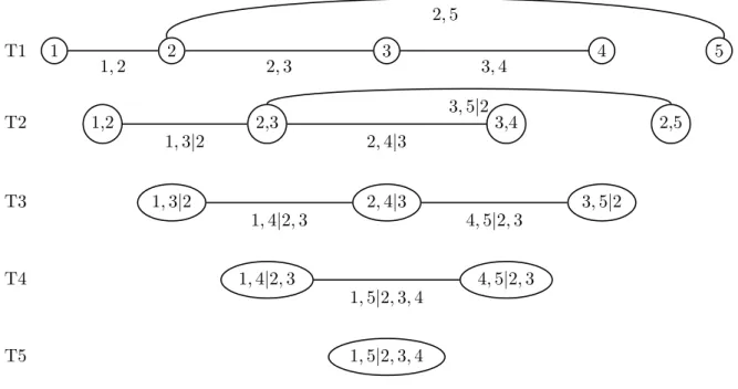
3.2 Regular Vine Representation . . . . 29
3.3 Vine Array Representation . . . . 32
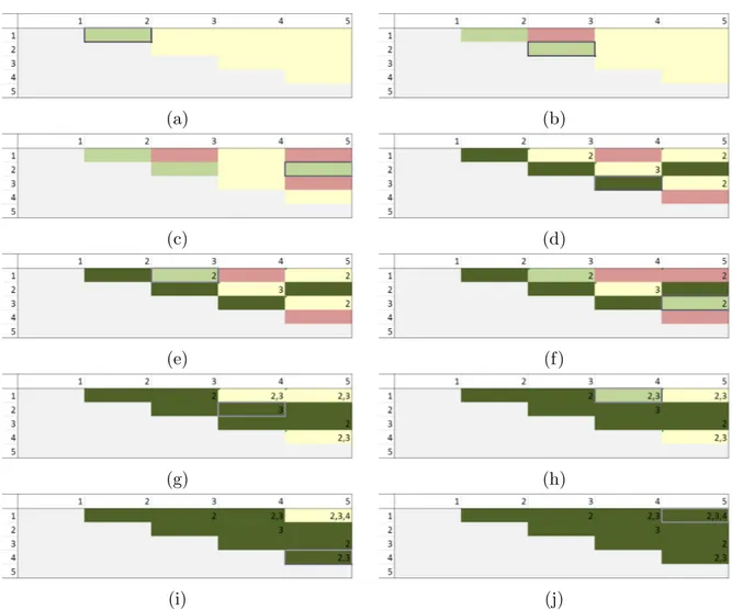
3.4 Matrix Representation . . . . 33
3.5 Conclusion . . . . 35
3.A Proofs . . . . 38
3.B Conditional Distributions . . . . 40
3.C Algorithms . . . . 41
4 Model Selection for Pair-Copula Constructions 45 4.1 Model Selection . . . . 45
4.1.1 Sequential Model Selection . . . . 46
4.1.2 Alternative Model Selection Techniques . . . . 47
4.2 Parameter Reduction Approach . . . . 48
4.3 Empirical Example . . . . 52
4.4 Conclusion . . . . 55
4.A Conditional Coverage Test . . . . 56
4.B Supplementary Results for the Empirical Example . . . . 57
5 Dependence Modeling for L´ evy Processes 61 5.1 L´evy Processes . . . . 61
5.1.1 Definition and Properties . . . . 62
5.1.2 L´evy Subordinators . . . . 68
5.2 L´evy Copulas . . . . 71
5.2.1 Definition and Properties . . . . 71
5.2.2 Parametric L´evy Copula Families . . . . 74
6 The Pair-L´ evy Copula Construction 75 6.1 Pair-L´evy Copulas . . . . 75
6.1.1 Technical Part . . . . 76
6.1.2 Pair-L´evy Copula Construction . . . . 78
6.2 Simulation and Estimation . . . . 83
6.2.1 Simulation . . . . 83
6.2.2 Maximum Likelihood Estimation . . . . 84
6.3 Simulation Study . . . . 88
6.4 Non-Gaussian Ornstein-Uhlenbeck Processes . . . . 89
6.4.1 Univariate Ornstein-Uhlenbeck Processes . . . . 91
6.4.2 Multivariate Ornstein-Uhlenbeck Processes . . . . 92
6.5 Overview of Further Applications . . . . 93
6.5.1 Operational Risk Modeling . . . . 94
6.5.2 Subordination of L´evy Processes . . . . 94
6.5.3 Modeling of Multivariate Volatility Indices . . . . 95
6.5.4 Stochastic Volatility Modeling . . . . 95
6.6 Conclusion . . . . 97
6.A Explicit 3-Dimensional Clayton PLCC . . . . 98
6.B Proofs . . . . 98
6.C Results of the Simulation Study . . . 103
6.D Algorithms . . . 110
7 Summary 113
List of Tables 115
List of Figures 117
Bibliography 120
List of Symbols and Abbreviations
# number of elements of a set; 29
∗ convolution; 65
h· , ·i inner product h x, y i = P
dj=1
x
jy
j; 65
∨ maximum; 42
∧ minimum; 42
× Cartesian product; 6
⊗ generalized product; 76
f
#µ push forward measure of measurable function f and measure µ; 76
1
( · ) indicator function; 18 B (R
d) Borel σ-algebra of R
d; 62 C copula function; 6
c copula density; 16 C
nempirical Copula; 17 C L´evy copula function; 72 c L´evy copula density; 85
F b
jnmarginal empirical distribution function; 17 (γ, Σ, ν) characteristic triplet; 66
λ
llower tail dependence coefficient; 15 λ
uupper tail dependence coefficient; 16 M Fr´echet-Hoeffding upper bound; 7 N natural numbers; 63
N extended natural numbers; 66 ν L´evy measure; 65
(Ω, F , P ) probability space; 62
PCC pair-copula construction; 3
ϕ
ξcharacteristic function of the probability measure ξ;
65
Π independence copula; 7
PLCC pair-L´evy copula construction; 4 PRM Poisson random measure; 66 Ran( · ) range of a function; 6
R
dd-dimensional Euclidean space; 6 R
d+non-negative elements of R
d; 69
R
dextended d-dimensional Euclidean space [ −∞ , ∞ ]
d; 6
R
d+non-negative elements of R
d; 72 ρ
SSpearman’s rho; 15
S
d+symmetric non-negative definite d × d matrix; 65 τ Kendall’s tau; 15
U tail integral; 71
u
ni,jpseudo observation; 17 V regular vine; 29
VaR
αvalue at risk: for a random variable X we define the VaR
αby P (X < VaR
α) = 1 − α; 52
W Fr´echet-Hoeffding lower bound; 7
(X
t)
t∈R+stochastic process, where X
t= X(t) denotes the re-
spective random variable at time t; 62
Chapter 1 Introduction
Measuring, describing, and modeling the dependence structure between different ran- dom events is at the very heart of statistics. Therefore, a broad variety of different dependence concepts have been developed in the past. The most famous concept is the correlation coefficient of Bravais-Pearson, and in many applied fields it is even common to express the dependence of a multivariate random variable solely by its correlation.
However, the correlation coefficient has various drawbacks and is only a measure of linear dependence. In order to model the full dependence structure of multivariate ran- dom variables, one needs to go beyond dependence measures. Copula theory offers the possibility to model the entire dependence structure of a multivariate random variable separately from its margins. This approach has been thoroughly investigated in recent publications, however, most work has been done in the 2-dimensional case and for static random variables. Using this concept in a high-dimensional or continuous-time setting is still challenging and the focus of this dissertation.
During the last two decades, we have observed a huge increase in scientific publica-
tions and conferences on dependence modeling. Embrechts (2009) explains this increas-
ing attention by the application of the copula concept in the financial sector, driven by
renewed regulatory guidelines and new financial products. The recent financial crisis
has illustrated that risk management is another area where sound dependence modeling
is essential. Throughout the crisis, it has become obvious that there are no risk free
investments. Housing prices may decline, banks and insurance companies can file for
bankruptcy, and even government bonds of developed countries and bank deposits are
not perfectly save. Thus, common sense suggests to diversify a portfolio in order to
avoid severe losses. However, the quantification of the risk exposure of a well-diversified
portfolio requires a thorough modeling of the dependence structure between the single
assets. That is why we need flexible and tractable high-dimensional dependence models
that account for the dependence between the different assets. These models enable us
to provide correct risk forecasts for the regulator and to base portfolio rebalancing de-
cisions on correct risk scenarios. In particular, we need dependence concepts that are
flexible enough to account for the joint behavior of assets in times of crises. There-
fore, dependence modeling is an important field in financial risk management. Besides
the numerous challenges, the enormously increased computational power as well as the
improved quality and availability of financial data constantly improves the modeling
−4 −3 −2 −1 0 1 2 3 4
−4
−3
−2
−1 0 1 2 3 4
X1 X2
(a)
−4 −3 −2 −1 0 1 2 3 4
−4
−3
−2
−1 0 1 2 3 4
X2 X3
(b)
−4 −3 −2 −1 0 1 2 3 4
−4
−3
−2
−1 0 1 2 3 4
X1 X3
(c)
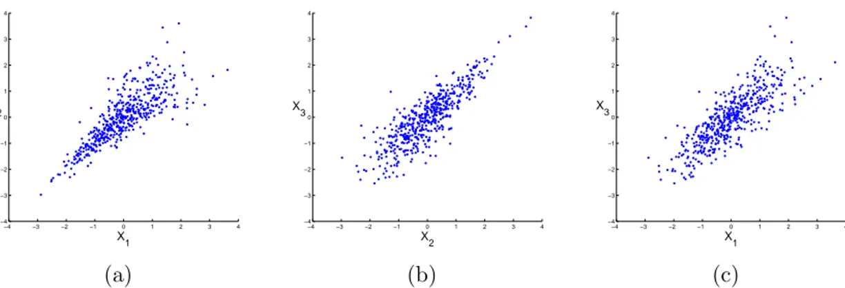
Figure 1.1: The three different plots show realizations of a 3-dimensional random variable with standard normally distributed margins. All bivariate margins have the same correlation coefficient; however, major differences in the joint behavior of the extremes are obvious. The underlying dependence structure is a pair- copula construction.
procedures. Overall, risk management is facing massive challenges and the constant improvement of the flexibility of the dependence models as well as the continuous ad- justment of the high-dimensional dependence concepts is only a small part in a sound risk management process. Nevertheless, poor dependence models can lead to dramatic misjudgments on the risk exposure of well-diversified portfolios, and therefore, with this dissertation, we intend to provide new tools to further improve dependence modeling.
Outline and Summary
This dissertation is divided into two parts. In the first part (Chapter 2-4), we focus
on modeling the dependence structure for static random variables in a high-dimensional
setting. Figure 1.1 illustrates why the correlation coefficient concept is not sufficient to
describe the full dependence structure of a multivariate random variable. All univariate
margins of this 3-dimensional random variable are standard normally distributed, and
all bivariate margins, which are visualized in the plot, have the same correlation coeffi-
cient; however, the joint behavior in the plots is quite different. In Figure 1.1a, extreme
negative values in the first dimension tend to occur at the same time as extreme negative
values in the second dimension, whereas in Figure 1.1b, we see a different behavior. Ex-
treme positive values occur at the same time, and the dependence of the strong negative
values is less distinct. Figure 1.1c shows neither a strong dependence in the extreme
positive nor in the extreme negative values. These differences in the behavior of the ex-
tremes can have severe consequences in many applications on the overall risk exposure,
and this problem is even more pronounced in higher dimensions as the correlation matrix
only provides insufficient information on the bivariate margins. Copula theory offers the
possibility to overcome most of the drawbacks of the correlation coefficient since this
theory provides all information on the dependence structure. Unfortunately, most of
the existing high-dimensional parametric copulas are not flexible enough to model a de- pendence structure like in Figure 1.1. A very promising approach to create flexible and tractable high-dimensional parametric copulas in arbitrary dimensions is the pair-copula construction (PCC) of Aas et al. (2009). This theory is based on the seminal work of Joe (1997), and the structure of a pair-copula constructions is usually visualized by the concept of regular vines, which has been developed by Bedford and Cooke (2002). How- ever, the implementation of estimation and simulation algorithms requires a different representation. Furthermore, the number of parameters in the pair-copula construction increases quadratically with the dimension and it is not evident that we need all of the parameters within the pair-copula construction. Therefore, the two main contributions of the dissertation to this field are
(i) the introduction of a new representation for pair-copula structures that is straight- forward to interpret and can be easily implemented in pair-copula algorithms, (ii) the development of a new parameter reduction technique that crucially reduces the
number of parameters in the pair-copula construction in order to avoid overfitting and to keep the model tractable in high dimensions.
The second part of the dissertation (Chapter 5-6) focuses on dependence modeling for continuous-time processes. The increasing availability of high frequency data and non- equidistantly spaced observations demand for continuous-time concepts. Furthermore, it can be useful to model equidistant data by an underlying continuous-time process, which is only observed at a discrete time grid. Compared to the static situation, continuous- time dependence modeling is still in its infancy. The contributions of the dissertation to this area of dependence modeling are
(iii) the development of a flexible, high-dimensional, parametric dependence concept for continuous-time stochastic processes,
(iv) the derivation of simulation and estimation techniques for this new dependence model.
We transfer some of the ideas from classical dependence modeling to the continuous-time setting. In particular, we use the intuition of the pair-copula construction techniques and develop a generalization of this concept for the L´evy copula framework of Kallsen and Tankov (2006).
This dissertation is structured as follows:
In Chapter 2, we recall the basics of copula theory. We fix the notation for the following
chapters and state Sklar’s theorem, the starting point in copula theory. Furthermore, we
recall the definitions of important parametric copula families. Copula based dependence
measures of bivariate random variables are recapitulated in Section 2.3, and in the
subsequent section, we discuss parametric and semi-parametric estimation techniques
for copulas. In Section 2.5, we recall one of the most powerful goodness-of-fit tests for
dependence structures. This test will play an important role in the parameter reduction
procedure that we introduce in Chapter 4.
Chapter 3 reviews the pair-copula construction framework. In Section 3.1, we sum- marize two different ways to introduce and interpret pair-copula constructions. These two approaches help to clarify the role of the controversial simplifying assumption in Subsection 3.1.3. We describe two different procedures to represent the structure of a pair-copula in the following sections. Furthermore, we discuss the advantages and draw- backs of these two pair-copula representations. Finally, in Section 3.4, we propose a new representation that overcomes some of the drawbacks of the existing ones.
A discussion of model selection procedures for the pair-copula construction is given in Chapter 4. Section 4.1 presents different heuristics to fit a pair-copula model to a data set. In the following, we focus on the sequential model selection approach of Subsection 4.1.1. Since pair-copula models can get very complex with increasing dimen- sions, we introduce a new parameter reduction technique in Section 4.2, which helps to avoid redundant parameters in the pair-copula construction process. We show that parameter reduced pair-copula models offer a flexible and low-parametric framework for high-dimensional dependence modeling. In the subsequent section, we illustrate how this parameter reduction technique works for a multivariate set of equity return data.
In Chapter 5, we discuss dependence modeling for stochastic processes. Therefore, we review the concept of L´evy processes in Section 5.1. This short summary is by far not exhaustive, but we fix the notation and recall some of the most important theorems for L´evy processes. Dependence modeling for these processes is discussed in the second part of the chapter. There, we review the concept of L´evy copulas that we use in the subsequent chapter. L´evy copulas model the jump dependence of L´evy processes. This is particularly important in many applications since L´evy copulas allow to model the dependence of sudden large movements in stochastic processes.
In Chapter 6, we transfer the pair-copula construction concept of Chapter 3 to the continuous-time setting of Chapter 5. That is, we develop a pair construction concept for L´evy copulas. In this concept, we assemble bivariate L´evy copulas and bivariate distributional copulas to one high-dimensional L´evy copula. This construction approach is introduced in Section 6.1. In the following section, we develop simulation techniques for dependent L´evy processes, based on the pair-L´evy copula construction (PLCC).
Furthermore, we provide maximum likelihood estimators for these continuous-time de-
pendence structures. In Section 6.3, we evaluate these new procedures in a simulation
study. In the following sections, we show how to apply the PLCC concept to multivariate
Ornstein-Uhlenbeck processes and give an outlook on further applications.
Chapter 2
Dependence Modeling with Copulas
Modeling the dependence structure between different events is one of the fundamental challenges in statistics. In applications, one is seldom confronted with one single source of uncertainty and the dependence structure between the different sources can have a tremendous effect on the overall risk exposure. This is a well-recognized fact especially in financial and actuarial applications. See, e.g., Genest et al. (2009a), McNeil et al.
(2005), Cherubini et al. (2004), and Panjer (2006). However, thorough dependence modeling is also important in many other areas like hydrology, engineering, operations research, economics, and biostatistics, see, e.g., Genest and Favre (2007) and Genest et al. (2009a).
The correlation coefficient of Bravais-Pearson is the most prominent dependence con- cept. However, as discussed, e.g., in Embrechts et al. (2002), the correlation coefficient has severe drawbacks for non-elliptical random variables and is only a measure of linear dependence. For a survey on dependence measures that are invariant under monotonic transformations and often more appropriate than the correlation, we refer to Schmid et al. (2010). In this chapter, we review the copula concept of Hoeffding (1940) and Sklar (1959) which has been rediscovered and expanded, e.g., by Joe (1997), Nelsen (2006), and references therein. Copulas go beyond dependence measures and provide a sound framework for general dependence modeling. They separate the margins and the dependence structure of any multivariate distribution. This result is important to estimate, understand, and interpret the dependence structure in a given set of data. Fur- thermore, this concept offers the possibility to combine arbitrary marginal distributions to a valid multivariate distribution function with a specific dependence structure. This is essential for multivariate modeling, since we can use sophisticated univariate models for any margin and combine them with a copula. Moreover, the separation of the depen- dence structure and the margins offers the possibility to estimate a parametric model for the multivariate distribution in two steps. That is, one estimates the parameters of the univariate marginal models in a first step and continues by estimating the dependence structure in a second step. This is a very important feature, since even the estima- tion of high-dimensional distributions becomes feasible in this sequential framework. In addition, simulation of random variables is straightforward within the copula concept.
The standard references for copula theory are Joe (1997) and Nelsen (2006). Durante
and Sempi (2010) give a historical introduction to the topic and provide an extensive
list of further references. The application of copula theory to finance is discussed, e.g., in McNeil et al. (2005), Cherubini et al. (2004), and Cherubini et al. (2012). Mai and Scherer (2012) give a broad overview on simulation techniques.
This chapter is structured as follows. In the first section, we give a short introduc- tion to copula theory. Then, we discuss methods to create valid copula functions and give prominent examples of parametric copula families that we apply in the subsequent chapters. In the third section, we present dependence measures for bivariate random variables that are solely based on the underlying copula. In the fourth section, we discuss different estimation procedures for an underlying parametric copula. Finally, we recall goodness-of-fit procedures to decide whether we have found an adequate dependence model for a given set of data.
2.1 Definition, Properties, and Sklar’s Theorem
In this section, we give a brief introduction to copula theory. We state some of the well-known properties of copula functions that we need in the subsequent chapters. For a more detailed introduction and the proofs of the given results, we refer to Joe (1997) and Nelsen (2006). Furthermore, with Sklar’s theorem, we recall the central result in copula theory that explains the key role of copula functions in dependence modeling. In the next definition, we formally define copulas.
Definition 2.1 A d-dimensional distribution function C(u
1, . . . , u
d) : [0, 1]
d→ [0, 1], where the margins satisfy C
j(u
j) = C(1, . . . , 1, u
j, 1, . . . , 1) = u
jfor all u
j∈ [0, 1] and j = 1, . . . , d, is called a copula.
Obviously, the condition on the margins assures that the copula is a distribution func- tion with uniform margins. Sklar’s Theorem is the starting point in copula theory. It shows how we can decompose any multivariate distribution function into the marginal distribution functions and a copula that contains the dependence structure. The the- orem was first given in Sklar (1959) and is also stated, e.g., in Nelsen (2006, Theorem 2.10.9).
Theorem 2.2 Let F
1,...,dbe a d-dimensional distribution function with marginal distri- bution functions F
1, . . . , F
d. Then there exists a copula C such that for all x ∈ R
d,
F
1,...,d(x
1, . . . , x
d) = C(F
1(x
1), . . . , F
d(x
d)). (2.1)
If F
1, . . . , F
dare all continuous, then C is unique. Otherwise, C is uniquely determined
on the Cartesian product of the ranges of the marginal distribution functions Ran(F
1) ×
. . . × Ran(F
d). Conversely, if C is a copula and F
1, . . . , F
dare distribution functions,
then the function F
1,...,ddefined by Equation (2.1) is a d-dimensional distribution function
with margins F
1, . . . , F
d.
2.1 Definition, Properties, and Sklar’s Theorem
In this work, we focus on continuous margins only. For a treatment of copula theory with discrete marginal distributions, we refer to Genest and Neˇslehov´a (2007). Next, we discuss functions of special importance in copula theory. The Fr´echet-Hoeffding upper bound M, the Fr´echet-Hoeffding lower bound W , and the independence copula Π are given by
M (u) = min(u
1, . . . , u
d), (2.2)
Π(u) = u
1· . . . · u
d, (2.3)
W (u) = max(u
1+ . . . + u
d− d + 1, 0). (2.4) Note that the Fr´echet-Hoeffding upper bound M and the independence copula Π are copulas in arbitrary dimensions, whereas the Fr´echet lower bound W is only in the bivariate case a copula function. The Fr´echet-Hoeffding bounds are pointwise bounds for any copula function. This is shown, for instance, in Nelsen (2006, Theorem 2.10.12).
Proposition 2.3 If C is any copula function, then for every u ∈ [0, 1]
d,
W (u) ≤ C(u) ≤ M (u) (2.5)
holds.
Note that even for d > 2, where the Fr´echet-Hoeffding lower bound W is not a copula, these inequalities are best possible. Furthermore, M , Π, and W have a special interpre- tation, as given, e.g., in Nelsen (2006, Theorem 2.5.5, Theorem 2.10.14), whenever they are copulas.
Proposition 2.4 For d ≥ 2, let X
1, . . . , X
dbe continuous random variables. Then (i) X
1, . . . , X
dare independent if and only if the copula of X
1, . . . , X
dis Π,
(ii) each of the random variables X
1, . . . , X
dis almost surely a strictly increasing func- tion of any of the others if and only if the copula of X
1, . . . , X
dis M .
For d = 2, let X
1, X
2be continuous random variables. Then
(iii) X
1is almost surely a strictly decreasing function of X
2if and only if the copula of X
1, X
2is W .
In more than two dimensions, the properties of the Fr´echet-Hoeffding upper and lower
bound are very different. This is due to the fact that positive and negative dependencies
are not comparable anymore. It is possible, for example, to have a collection of random
variables X
1, . . . , X
dsuch that each of these random variables is an increasing function
of any of the others. This is not possible for negative dependencies and more than
two random variables. Suppose that X
1is a decreasing function of X
2and X
2is a
decreasing function of X
3as well. Then, the variable X
1has to be an increasing function
of X
3. Another important and well-known property of any copula is given in the next
proposition, see, e.g., Nelsen (2006, Theorem 2.10.7).
Proposition 2.5 Let C be a d-dimensional copula. Then for every u and v in [0, 1]
d,
| C(v) − C(u) | ≤ X
dj=1
| v
j− u
j| .
Hence, C is uniformly continuous on [0, 1]
d.
There are different kinds of symmetry for copula functions. See, e.g., Nelsen (2006, Chapter 2.7). Here, we recall the definition of permutation symmetry, which is a neces- sary condition on the copula of exchangeable random variables.
Definition 2.6 Let C be a d-dimensional copula. We say C is permutation-symmetric if
C(u
1, . . . , u
d) = C(u
τ(1), . . . , u
τ(d)) for any permutation τ and any u
1, . . . , u
d∈ [0, 1]
d.
Thus, permutation-symmetry is closely related to the concept of exchangeability for random variables.
2.2 Parametric Copula Families
We are not only interested in theoretical properties of copula functions, but we want to
apply this theory to a given data set as well. Therefore, we discuss different construction
methods for d-dimensional, parametric dependence structures. Furthermore, we recall
the definition of selected copula families that we need in the following chapters. Note
that this is by no means exhaustive. Especially in two dimensions, there are plenty
of different copulas families. For a thorough discussion, we refer to Joe (1997), Nelsen
(2006), and references therein. However, there are only few copula models that are
flexible enough to represent the dependence structure of high-dimensional data. The
most prominent ones are the Gauss and t copula being easy to estimate and widely used
in applications. In some cases, however, these dependence structures fail to model
desirable dependence properties. Nevertheless, we use them as benchmarks for the
high-dimensional copula model in Chapter 3. Another approach to build multivariate
copulas is based on the extension of bivariate Archimedean copulas. Unfortunately,
these copulas lack the desired flexibility in higher dimensions. In the third part of this
section, we discuss a hierarchical procedure to overcome this problem. Therefore, we
combine lower-dimensional Archimedean copulas such that the resulting structure is a
valid d-dimensional copula.
2.2 Parametric Copula Families
2.2.1 Implicit Copula Families
Here, we present a way to define parametric copula families by extracting the dependence structure of a known multivariate distribution. The next corollary shows how to invert Sklar’s theorem to define parametric copula families in d dimensions. This corollary is already stated, e.g., in Nelsen (2006, Corollary 2.10.10).
Corollary 2.7 Let F
1,...,dbe a d-dimensional distribution function, where F
1, . . . , F
ddenote the continuous marginal distribution functions, and let C be the corresponding copula. We denote the marginal quasi-inverses, see Nelsen (2006, Definition 2.3.6), by F
1−1, . . . , F
d−1. Then, we have for any u ∈ [0, 1]
dC(u
1, . . . , u
d) = F
1,...,d(F
1−1(u
1), . . . , F
d−1(u
d)).
This relation is particularly interesting for the class of elliptical distributions, since the univariate margins as well as the multivariate distribution function are well-known. See, e.g., Fang et al. (1990). Furthermore, the resulting copulas are quite flexible dependence models. These elliptical copulas can be used to combine arbitrary margins and create new multivariate distribution functions. In the next example, we give the definition of the best known elliptical copula.
Example 2.8 Let Φ
1,...,dbe the distribution function of the multivariate normal distri- bution with zero mean and correlation matrix R. We denote the distribution function of the univariate standard normal distribution by Φ, and define the d-dimensional Gauss copula by
C(u
1, . . . , u
d) = Φ
1,...,d(Φ
−1(u
1), . . . , Φ
−1(u
d)).
The Gauss copula extracts the dependence structure from the multivariate normal dis- tribution. It is uniquely defined by the correlation matrix and thus has d(d − 1)/2 parameters. Hence, it offers a certain flexibility and is widely applied. We use the Gauss copula as a benchmark model for the more advanced multivariate copula models that we discuss in Chapter 3. In financial applications, however, it is often observed that the dependence of the extreme events is stronger than suggested by the Gauss copula.
Therefore, we state the definition of the t copula in the next example. For the definition of the multivariate t-distribution t
1,...,d, we refer to Fang et al. (1990, Example 2.5).
Example 2.9 Let t
1,...,dbe the distribution function of a vector X ∼ t
1,...,d(ν, 0, R), where R is a correlation matrix and ν > 0. We denote the univariate standard t-distribution with ν degrees of freedom by t, and we define the d-dimensional t copula by
C(u
1, . . . , u
d) = t
1,...,d(t
−1(u
1), . . . , t
−1(u
d)).
In contrast to the Gauss copula, the t copula has an additional parameter to control
for the dependence of the extreme events. This makes the t copula more suitable for
financial application. However, the t copula is symmetric in the sense that extreme positive and extreme negative events are modeled equivalently. Furthermore, there is only one parameter for the dependence of all extreme events, which might not be enough for high-dimensional dependence structures. The definitions of these two copulas can be found, e.g., in McNeil et al. (2005, Chapter 5).
2.2.2 Archimedean Copulas
Besides the implicit copulas, the class of Archimedean copulas is one of the most popular families in parametric dependence modeling. In contrast to implicit copula families, we do not need well-known multivariate distribution functions to create a new copula family.
Archimedean copulas are uniquely defined by a generating function. The generator of a 2-dimensional Archimedean copula is a convex, continuous, and strictly decreasing function ϕ : [0, 1] 7→ [0, ∞ ], such that ϕ(1) = 0. The following theorem, stated, e.g., in Nelsen (2006, Section 4.1), shows how to use the generator to define a valid copula.
Theorem 2.10 Let ϕ be a generator function and denote by ϕ
[−1]the pseudo inverse
ϕ
[−1](t) =
( ϕ
−1(t) 0 ≤ t < ϕ(0), 0 ϕ(0) ≤ t ≤ ∞ . Then, the function C : [0, 1]
27→ [0, 1]
C(u, v) = ϕ
[−1](ϕ(u) + ϕ(v)) (2.6)
is a copula.
In the next example, we present three of the most popular Archimedean copulas that we are going to use in the subsequent chapters. For more information on these copulas and additional Archimedean families, we refer to Nelsen (2006).
Example 2.11 In this example, we give the generator and the copula function of selected bivariate Archimedean copulas.
• Clayton copula (Clayton, 1978): For θ ∈ [ − 1, ∞ ) \{ 0 } , the Clayton copula is given by
C(u, v) = max { u
−θ+ v
−θ− 1, 0 }
−1θ, (2.7)
with generator
ϕ(t) = 1
θ (t
−θ− 1).
For θ = 0, we set C = Π.
• Gumbel copula (Gumbel, 1960): For θ ∈ [1, ∞ ), the Gumbel copula is defined as C(u, v) = exp
− ( − log(u))
θ+ ( − log(v))
θ1θ, (2.8)
2.2 Parametric Copula Families
with generator
ϕ(t) = ( − log(t))
θ.
• Frank copula (Frank, 1979): For θ ∈ ( −∞ , ∞ ) \{ 0 } , the Frank copula is defined as C(u, v) = − 1
θ log
1 + (e
−θu− 1)(e
−θv− 1) e
−θ− 1
, (2.9)
with generator
ϕ(t) = − log
e
−θt− 1 e
−θ− 1
. Again, we set C = Π for θ = 0.
The concept of Archimedean copulas can be generalized to the multivariate case.
The definition of the multivariate Archimedean copula is straightforward. However, we need to impose additional assumptions on the generator to guarantee for a valid copula function. This is formalized in Nelsen (2006, Theorem 4.6.2).
Theorem 2.12 Let ϕ : [0, 1] 7→ [0, ∞ ] be a continuous strictly decreasing function such that ϕ(0) = ∞ and ϕ(1) = 0, and let ϕ
−1denote the inverse of ϕ. We define a function C : [0, 1]
d7→ [0, 1] by
C(u) = ϕ
−1(ϕ(u
1) + . . . + ϕ(u
d)) .
The function C is a copula for all d ≥ 2 if and only if ϕ
−1is completely monotonic on [0, ∞ ), that is, it is continuous and has derivatives of all orders that alternate in sign for any t ∈ (0, ∞ ).
For necessary and sufficient conditions on the generator for a fixed dimension d, we refer to McNeil and Neˇslehov´a (2009). Note that these multivariate copulas are permutation- symmetric. This implies that all lower-dimensional margins of the copula have the same dependence structure. In particular, models based on multivariate Archimedean copulas have equicorrelated ranks.
2.2.3 Hierarchical Archimedean Copulas
Two-dimensional Archimedean copulas constitute a very important class in dependence
modeling. Some of the best known copula families are Archimedean and this property
has many theoretical and practical advantages. As shown in the preceding section,
generalizations to the multivariate case (d ≥ 3) are possible. However, the property of
permutation-symmetry is a severe restriction in more than two dimensions. Usually, this
symmetry is not tenable when dealing with a high-dimensional set of data. Joe (1997)
introduces the idea of a hierarchical construction method to define multivariate copulas
by nesting different lower-dimensional Archimedean copulas. With this approach, one
can partially overcome the permutation-symmetry in high-dimensional copula models.
C
3;1C
2;1C
1;11 2 3 4
(a)
C
2;1C
1;1C
1;21 2 3 4 5
(b)
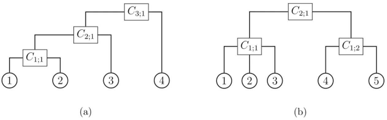
Figure 2.1: This plot shows an example of two different hierarchical Archimedean copula structures
The idea in Joe (1997) is straightforward. First, one models the dependence between the first and second dimension with the bivariate Archimedean copula C
1;1. In the next step, one defines z
1,2= C
1;1(u
1, u
2) and combines this new variable with the untransformed variable u
3of the third dimension by the Archimedean copula C
2;1. Then, one defines z
1,2,3= C
2;1(z
1,2, u
3) and we can iterate this procedure until all variables are included.
This approach is visualized in Figure 2.1a with four variables. The dependence function is given by
C
1,2,3,4(u
1, u
2, u
3, u
4) =
= C
3;1(C
2;1(C
1;1(u
1, u
2), u
3), u
4)
= ϕ
[−1]3;1ϕ
3;1◦ ϕ
[−1]2;1ϕ
2;1◦ ϕ
[−1]1;1ϕ
1;1(u
1) + ϕ
1;1(u
2)
+ ϕ
2;1(u
3)
+ ϕ
3;1(u
4) , where we denote the generator of C
i;jby ϕ
i;j. A sufficient condition for C
1,2,3,4to be a copula is that all inverse generator functions are completely monotonic, and furthermore, the composition of the generator functions ϕ
3;1◦ ϕ
[−1]2;1and ϕ
2;1◦ ϕ
[−1]1;1have to be completely monotonic as well, see Joe (1997, Chapter 4).
Different nestings strategies also lead to valid multivariate copulas. A 5-dimensional example is illustrated in Figure 2.1b. In this case, the copula is given by
C
1,2,3,4,5(u
1, . . . , u
5) = C
2;1(C
1;1(u
1, u
2, u
3), C
1;2(u
4, u
5))
= ϕ
[−1]2;1ϕ
2;1◦ ϕ
[−1]1;1ϕ
1;1(u
1) + ϕ
1;1(u
2) + ϕ
1;1(u
3) + ϕ
2;1◦ ϕ
[−1]1;2ϕ
1;2(u
4) + ϕ
1;2(u
5)
,
where all inverse generator functions as well as ϕ
2;1◦ ϕ
[−1]1;1and ϕ
2;1◦ ϕ
[−1]1;2have to be completely monotonic. This procedure can be extended easily to arbitrary dimensions.
However, the notation gets involved, and therefore we refer to Savu and Trede (2010)
for a general treatment. Choosing an adequate nesting structure is treated in Okhrin
(2007), simulation techniques for hierarchical Archimedean copulas are given in Whelan
2.3 Dependence Measures
(2004), McNeil (2008), and Hofert (2008). The density for the general case is derived in Savu and Trede (2010).
Hierarchical Archimedean copulas are popular for several reasons. They overcome the problem of permutation-symmetry, the connection to other areas in probability theory like Laplace transforms is appealing, and the hierarchical structure often has a nice interpretation. In financial applications, for example, the dependence of the assets in one sector can be modeled on the first level and the dependence between the different sectors on a second. However, there are also severe drawbacks of this method. For any hierarchical structure and any selection of Archimedean copulas, the conditions on the composite generator functions have to be verified separately. Furthermore, these conditions can be very restrictive. In the hierarchy of Figure 2.1b, for example, it is not possible to use a Gumbel copula for C
1;1and a Clayton copula for C
2;1, see Savu and Trede (2010). The conditions are only easy to verify if all Archimedean copulas in the hierarchy belong to a special Archimedean family. For instance, if all copulas in the structure are of Gumbel type, of Clayton type, or of Frank type one only has to check that the dependence parameters decrease with the hierarchy level (Aas and Berg, 2009). That is, for the hierarchy in Figure 2.1b, we need to guarantee that θ
2;1< θ
1;1and θ
2;1< θ
1;2. However, the restriction to one copula family for all copulas in the hierarchy limits the applicability of the concept strongly. Finally, hierarchical Archimedean copulas are not the only high-dimensional dependence models that overcome permutation-symmetry.
The multivariate Gauss and t copula, as well as the pair-copula construction of Chapter 3 are in general not permutation-symmetric. Furthermore, in the model comparison of Fischer et al. (2009) and Aas and Berg (2009), hierarchical Archimedean copula models perform worse than competing dependence structures.
2.3 Dependence Measures
The copula framework is a most general dependence concept. It captures all infor- mation on the dependence structure of a random variable. However, the copula is a d-dimensional cumulative distribution function on [0, 1]
dand therefore hard to inter- pret. Furthermore, comparing the magnitude of dependence for different copulas might be ambiguous. Therefore, it is often advantageous to summarize the dependence struc- ture in a scalar valued dependence measure. The most famous dependence measure is the correlation coefficient ρ of Bravais-Pearson. But, as discussed, this measure has many drawbacks for non-elliptical dependence structures. In this section, we present three alternatives. These measures depend only on the underlying copula and not on the marginal distributions. This is a desirable property, since the margins do not influ- ence the dependence structure. In addition, the first two dependence measures are more robust to estimate than the correlation coefficient. Here, we focus on the bivariate case.
For generalizations to the d-dimensional case (d ≥ 3), we refer to Gaißer (2010), Schmid
et al. (2010), and references therein.
−4 −3 −2 −1 0 1 2 3 4
−4
−3
−2
−1 0 1 2 3 4
X Y
(a)
−4 −3 −2 −1 0 1 2 3 4
−4
−3
−2
−1 0 1 2 3 4
X Y
(b)
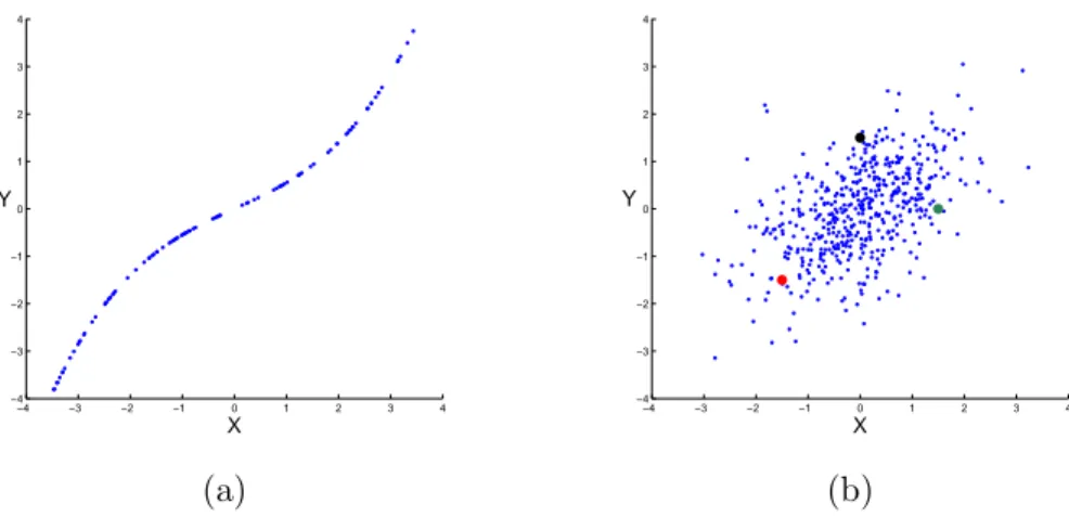
Figure 2.2: The plot on the left shows a deterministic relation between X and Y . In particular, every pair of two realizations is concordant. In the plot on the right, we have a realization of a bivariate normal distribution with a positive correlation coefficient, and there are more concordant than discordant pairs.
2.3.1 Measures of Concordance
In this section, we discuss two well-known bivariate measures of association that do not depend on the marginal distributions. There exists a broad variety of different bivariate dependence measures. For an overview on these, we refer to Nelsen (2006). Here, we recall briefly two selected measures of association that are particularly important in the subsequent chapters. To introduce these measures, we need to discuss the concept of concordance. Let (X, Y ) be a bivariate random variable. A pair of realizations (x
1, y
1) and (x
2, y
2) is concordant if x
1< x
2and y
1< y
2, or x
1> x
2and y
1> y
2. That is, if (x
1− x
2)(y
1− y
2) > 0. In Figure 2.2b, the red and the black points as well as the red and the green points are concordant. We say that (x
1, y
1) and (x
2, y
2) are discordant if x
1< x
2and y
1> y
2, or x
1> x
2and y
1< y
2. That is, if (x
1− x
2)(y
1− y
2) < 0. In Figure 2.2b, the black and the green observations are discordant. Figure 2.2 visualizes how we use the concordance concept to measure the dependence of random variables. Figure 2.2a shows a realization of a perfectly positively dependent random variable (X, Y ).
Here, all pairs are concordant. In Figure 2.2b, we have a non-deterministic dependence structure of a bivariate normal distribution with a positive correlation. In this case, we observe more concordant than discordant pairs. With this concept, we are able to introduce two different measures of association.
Kendall’s Tau
This dependence measure is introduced in Kendall (1938). Let (X
1, Y
1) and (X
2, Y
2)
be independent and identically distributed random variables with continuous marginal
2.3 Dependence Measures
distribution functions F
X(x), F
Y(y) and copula C. We define Kendall’s tau as
τ = P ((X
1− X
2)(Y
1− Y
2) > 0) − P ((X
1− X
2)(Y
1− Y
2) < 0) (2.10)
= 4 Z
[0,1]2
C(u, v)dC(u, v) − 1.
That is, Kendall’s tau gives the probability of concordance minus the probability of discordance. The second relation is proved, e.g., in Nelsen (2006).
Spearman’s Rho
Spearman’s rho is first mentioned in Spearman (1904) as a rank-based dependence mea- sure. Nelsen (2006) introduces this measure in the following way. Let (X
1, Y
1), (X
2, Y
2) and (X
3, Y
3) be independent and identically distributed random variables with continu- ous marginal distribution functions F
X(x), F
Y(y) and copula C. We define Spearman’s rho by
ρ
S= 3 (P ((X
1− X
2)(Y
1− Y
3) > 0) − P ((X
1− X
2)(Y
1− Y
3) < 0)) (2.11)
= 12 Z
[0,1]2
uv dC(u, v) − 3.
Interestingly, it is easy to show that Spearman’s rho is exactly the correlation coefficient between F
X(X) and F
Y(Y ). That is,
ρ
S= Cov(F
X(X), F
Y(Y )) p Var(F
X(X)) p
Var(F
Y(Y )) .
2.3.2 Tail Dependence
Kendall’s tau and Spearman’s rho measure the dependence on the whole range of the bivariate random variable (X, Y ). The tail dependence coefficient, on the contrary, is a measure for the dependence of extreme events. Again, we denote the marginal distribution functions by F
X(x), F
Y(y) and the copula by C. The lower tail dependence coefficient is given by
λ
l= lim
u0
P Y ≤ F
Y−1(u) X ≤ F
X−1(u)
(2.12)
= lim
u0
C(u, u)
u , (2.13)
and the upper tail dependence coefficient is λ
u= lim
u1
P Y > F
Y−1(u) X > F
X−1(u)
(2.14)
= 2 − lim
u1
1 − C(u, u)
1 − u . (2.15)
The representation of the tail dependence coefficient in terms of the copula in Equation (2.13) and (2.15) is derived, e.g., in Nelsen (2006, Section 5.4). See Frahm et al. (2005) for a survey of different estimators. Tail dependence is an important property in finance.
The Gauss copula has a tail dependence of zero and is therefore not appropriate in many situations. The t copula can model upper and lower tail dependence, where λ
u= λ
l. The next example presents a copula that has both upper and lower tail dependence. Furthermore, this copula can have different values for the upper and lower tail dependence coefficient.
Example 2.13 The BB1 copula family, introduced and discussed in Joe and Hu (1996, Example 5.1), is a parametric copula with different upper and lower tail dependence. In particular, the upper and lower tail dependence coefficients can be set independently of each other. The bivariate copula with parameters θ > 0 and τ ≥ 1 is defined by
C(u, v; θ, τ ) =
1 + (u
−θ− 1)
τ+ (v
−θ− 1)
ττ1−1θ.
The lower tail dependence coefficient is λ
l= 2
−1/(τ θ)and the upper tail dependence coefficient is λ
u= 2 − 2
1/τ.
For further measures of tail dependence in arbitrary dimensions, we refer to Schmid and Schmidt (2007).
2.4 Estimation
There are different ways to estimate the underlying copula for a given set of i.i.d data. In this section, we give a very brief overview and discuss the estimation procedure that we use in the subsequent chapters. For a survey of the different estimation procedures, we refer to Choro´s et al. (2010). We focus on maximum likelihood methods only, using that under absolute continuity assumptions the probability density f
1,...,dcan be decomposed into
f
1,...,d(x
1, . . . , x
d) = c(F
1(x
1), . . . , F
d(x
d)) Y
d i=1f
i(x
i), (2.16)
where f
1, . . . , f
dare the marginal densities and c is the copula density. The first possible
method is the straightforward maximum likelihood estimation of the full model. This
requires choosing a parametric model for the copula and the margins such that we can
2.4 Estimation
calculate the full likelihood function with respect to all parameters. That is, we specify the parameter vectors α
1, . . . , α
dof the margins and the parameter vector θ of the copula altogether. The problem of this method is that the number of parameters can be very large, even for moderate dimensions. Therefore, the optimization algorithm might be very slow or even computationally infeasible.
To overcome this problem, or at least to provide good starting values for the full max- imum likelihood method, Joe (1997) has suggested the inference functions for margins (IFM) approach. This is a sequential procedure where we estimate the marginal param- eters separately for every dimension. In a second step, we transform the observations (x
i,1, . . . , x
i,d)
i=1,...,nwith the estimated marginal distribution functions
u
IFMi,j= F
j(x
i,j; ˆ α
j),
for i = 1, . . . , n and j = 1, . . . , d. In the following, we treat the transformed variables (u
IFMi,1, . . . , u
IFMi,d)
i=1,...,nlike observations from the underlying copula and estimate the parameter vector θ by the maximum likelihood approach. This is conceptually the same as plugging in the marginal estimators into the likelihood function that is based on the density in Equation (2.16) and maximizing this likelihood function with respect to the copula parameters. Of course, it is not possible to apply the standard maximum likelihood results for the asymptotic properties of this sequential estimator. However, Joe (1997) proves consistency and asymptotic normality under the usual regularity con- ditions. This stepwise procedure reduces the complexity of the problem and makes estimation feasible even for high dimensions and complex marginal models. However, since the marginal distributions are unknown, we cannot guarantee to select the correct model for the margins and, as shown in Kim et al. (2007), misspecified margins can have a crucial effect on the estimator of the copula parameter.
The third method is similar to the IFM approach but it is based on nonparametric estimates of the margins. This excludes the possibility of misspecified margins and is particularly appropriate if the dependence structure is in the focus of the analysis.
We denote the one-dimensional empirical distribution function by F b
jnand define the pseudo-observations as
u
ni,j= n
n + 1 F b
jn(x
i,j), (2.17) for i = 1, . . . , n and j = 1, . . . , d. Note that we use the normalization n/(n + 1) to avoid problems at the boundaries of [0, 1]
d. Thus, the pseudo-observations are simply the rank of the observation in its dimension, normalized by 1/(n + 1). In the next step, we continue as in the IFM case. That is, we treat (u
ni,1, . . . , u
ni,d)
i=1,...,nas observations from the underlying copula and estimate the parameter vector θ with a standard maxi- mum likelihood approach. Genest et al. (1995) show that the semiparametric estimator is consistent and asymptotically normal. Kim et al. (2007) advocate the use of this estimation method if the marginal distributions are unknown.
A completely nonparametric way to estimate the copula is given in Deheuvels (1979).
We use the pseudo-observation of Equation (2.17) and define the empirical copula on
[0, 1]
das
C
n(u
1, . . . , u
d) = 1 n
X
n i=11
(u
ni,1≤ u
1, . . . , u
ni,d≤ u
d). (2.18) Note that C
nis not continuous and therefore not a copula function. Furthermore, one needs a large amount of data to get a good approximation of the underlying copula on [0, 1]
dby the empirical copula function. Thus, one of the main applications of the empirical copula is goodness-of-fit testing for parametric copula models.
2.5 Goodness-of-Fit
There are several different ways to evaluate the fit of a parametric copula for a given data set. A graphical analysis of the dependence structure should always be the first step. In two dimensions, scatter plots of the data can give a first hint on the depen- dence. However, in many cases, the influence of the marginal distributions conceals the underlying dependence structure. Therefore, it is advantageous to transform the orig- inal data and plot the pseudo-observations. Sometimes, these pseudo-observations are further transformed such that all univariate margins are standard normally distributed.
In this case, all margins have the same distribution and do not affect the scatter plot asymmetrically. By construction, scatter plots are particularly appropriate for two di- mensions. Nevertheless, in the multivariate case, we can apply the bivariate graphical methods on the 2-dimensional margins. A different graphical approach to evaluate the fit of a parametric copula is suggested by Genest and Rivest (1993). They transform the selected parametric copula C to the so called λ-function on [0, 1]. Then, they compare this function with its nonparametric estimate from the data. For further information and the definition of the theoretical and empirical λ-function, we refer to Genest and Rivest (1993) and Genest et al. (2009b).
Graphical evaluations are often suitable to discover a bad fit of the selected dependence model. Though, it is substantially more difficult to distinguish between a moderate and an excellent fit by these approaches. Furthermore, it is desirable to have a statistical framework to validate the intuition that we get from the graphical procedures. Therefore, we need goodness-of-fit tests to decide whether the selected copula can represent the dependence structure in a given data set adequately. We denote a parametric copula family by C = { C
θ: θ ∈ O} , where O is an open subset in R
p. The hypotheses for these goodness-of-fit tests are given by
H
0: C ∈ C , against H
a: C / ∈ C .
Recently, a large variety of different goodness-of-fit tests have been proposed. Fermanian
(2005) bases his goodness-of-fit on the density of the copula. A different procedure is
introduced in Breymann et al. (2003) and corrected in Dobri´c and Schmid (2007). This
approach is based on the Rosenblatt transformation, see Rosenblatt (1952). Genest
et al. (2009b) and Berg (2009) introduce further approaches. Moreover, they conduct
2.A Parametric Two-Level Bootstrap G-o-F Algorithm
extensive simulation studies on computer clusters to compare size and power of selected goodness-of-fit tests for different hypotheses and sample sizes. Genest et al. (2009b) focus on the bivariate case, whereas Berg (2009) applies the tests in d = { 2, 4, 8 } dimensions.
Here, we discuss one of the goodness-of-fit tests. This test performs particularly well in the power comparison of the simulation studies and we use this test in Section 4.2 in the bivariate case. We denote by θ
nan estimate of θ. The test is proposed in Genest and R´emillard (2008) and is based on the distance between the empirical copula C
n, see Equation (2.18), and the fitted copula C
θn∈ C . More formally, the distance is measured by the empirical process
C
n= √
n (C
n− C
θn) and the Cram´er-von Mises test statistic
S
n= Z
[0,1]d
C
n(u)
2dC
n(u).
As shown in Genest and R´emillard (2008) and noted in Genest et al. (2009b), the asymptotic distribution of the test statistic is highly complex and depends on the copula family under the null hypothesis. Moreover, it is not possible to tabulate critical values since these values depend on the true parameter θ of the underlying copula. Therefore, we have to use a parametric bootstrap procedure to calculate the p-value of the goodness- of-fit test. The validity of this parametric bootstrap is derived in Genest and R´emillard (2008).
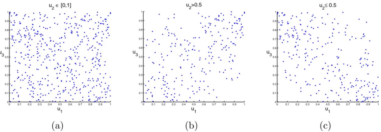
An example to illustrate the importance of goodness-of-fit tests is given in Figure 2.3.
In the plot 2.3a and 2.3b, we see realizations of a Frank and Gauss copula, respectively.
Both dependence structures have the same value of Kendall’s tau τ = 0.3. The corre- sponding empirical lambda functions are given in 2.3c. The blue empirical λ-function corresponds to the Frank copula. The red function corresponds to the Gauss copula. In this case, it is very difficult to distinguish between these dependence structures visually.
The goodness-of-fit test, on the contrary, is able to reveal the correct underlying copula in our example. The null hypothesis that the copula in the plot on the left is Gaussian is correctly rejected at a 1% level (p-value = 0.004), and the null hypothesis that the un- derlying copula in the plot in the middle is a Frank copula is correctly rejected (p-value
= 0.001) as well.
2.A Parametric Two-Level Bootstrap Goodness-of-Fit Algorithm
In this goodness-of-fit test, we compare the observed distance between the empirical
and the estimated parametric copula with the distance that we expect under the null
hypothesis. Therefore, we approximate the distribution of this distance under the null
with a parametric bootstrap procedure. The calculation procedure is provided in Genest
et al. (2009b, Appendix A), and the validity of the two-level bootstrap procedure is
0 0.1 0.2 0.3 0.4 0.5 0.6 0.7 0.8 0.9 1 0
0.1 0.2 0.3 0.4 0.5 0.6 0.7 0.8 0.9 1
u1 u2
(a)
0 0.1 0.2 0.3 0.4 0.5 0.6 0.7 0.8 0.9 1
0 0.1 0.2 0.3 0.4 0.5 0.6 0.7 0.8 0.9 1
u1 u2
(b)
0 0.1 0.2 0.3 0.4 0.5 0.6 0.7 0.8 0.9 1
−0.35
−0.3
−0.25
−0.2
−0.15
−0.1
−0.05 0
v λ
(c)
Figure 2.3: Pseudo-observations of a Frank (a) and Gauss (b) copula. Both copulas have a Kendall’s tau of τ = 0.3. The plot on the right shows the empirical lambda functions. The blue function corresponds to the data in (a) and the red function to (b).
derived in Genest and R´emillard (2008). In particular, the estimation step in line 11 is
time-consuming, since this estimation is conducted in every bootstrap iteration. On the
other hand, the computation procedure is appropriate for parallelization of the bootstrap
iterations. Note that, if the copula family under consideration can be evaluated efficiently
on u ∈ [0, 1]
2, it is not necessary to approximate the parametric copula at lines 3-4 and
12-13 in the bootstrap algorithm.
2.A Parametric Two-Level Bootstrap G-o-F Algorithm
Algorithm 1 Two-level parametric bootstrap goodness-of-fit test of Genest et al.
(2009b)
Input: pseudo-observations u
ni,j, i = 1, . . . , n and j = 1, . . . , d, parametric copula family C = { C
θ: θ ∈ Θ } , number of primary bootstrap samples N , number of secondary bootstrap samples m
Output: approximation of the p-value
1: define C
n(u) =
n1P
ni=11
(u
ni≤ u)
2: estimate θ with the maximum likelihood estimator θ
n3: generate random sample (y
1∗, . . . , y
∗m) from distribution C
θn4: approximate C
θn(u) by B
m∗(u) =
m1P
mi=11
(y
i∗≤ u)
5: compute S
n= P
ni=1
(C
n(u
ni) − B
m∗(u
ni))
26: for k = 1, . . . , N do
7: generate random sample (y
1,k∗, . . . , y
n,k∗) from distribution C
θn8: compute ranks (r
1,k∗, . . . , r
∗n,k) of (y
1,k∗, . . . , y
n,k∗)
9: compute pseudo-observations (u
∗1,k, . . . , u
∗n,k) = (
n+1r1,k∗, . . . ,
n+1rn,k∗)
10: define C
n,k∗(u) =
n1P
ni=11
(u
∗i,k≤ u)
11: estimate θ from (u
∗1,k, . . . , u
∗n,k) with the maximum likelihood estimator θ
∗n,k12: generate random sample (y
1,k∗∗, . . . , y
m,k∗∗) from distribution C
θn,k∗13: approximate C
θ∗n,k(u) by B
m∗∗(u) =
m1P
mi=11
(y
i,k∗∗≤ u)
14: compute S
n,k∗= P
ni=1
C
n,k∗(u
∗i,k) − B
∗∗m,k(u
∗i,k)
215: end for
16: p-Value = P
Nk=11