3.1 The Lagrange Formalism

Exercise 3 - Lagrange Formalism

3.1 The Lagrange Formalism

The Lagrange formalism is a mechanical method that allows to derive the equations of motion for a mechanical system. The big advantage of the Lagrange formalism over the Newton formulation, i.e. over F =m·x, lies in the analysis of the constraints. In fact,¨ constraints can be included much more easily in the Lagrange formalism.

3.1.1 Generalized Coordinates

Generalized coordinates are coordinates that can be used to describe a system uniquely.

Usually, they are stored in a vector ~q. Moreover, constraints reduce the system’s degrees of freedom and generalized coordinates can be adapted in order to describe them.

3.1.2 Holonomic vs. Non-holonomic Constraints

The constraints acting on a mechanical system can be divided into two groups. Non- holonomic constraints and holonomic constraints. The most general of the two con- straints’ types are non-holonomic constraints, which can be described by

f(~q,~q, t) = 0,˙

where~q is the generalized-coordinates vector. When no dependency on the general veloc- ities (state-variable vector derived) is present, the constraint is holonomic. This type of constraints can be once more subdivided into two subcategories: scleronomic constraints are discribed with

f(~q) = 0, and rheonomic constraints with

f(~q, t) = 0.

The reason why holonomic constraints are important is that they allow us reducing the number of variables used to describe a system. This is done by removing dependent variables. Let’s assume to have a constraint acting on a system described by n general coordinates qi:

f(q₁, . . . , q_n, t) = 0.

Then, only if a constraint is holonomic, we can write

q₁ =f(q₂, . . . , q_n). (3.1) Remark. If interested, recall the implicit function theorem.

In general, it holds

p=n−r,

where p is the number of degrees of freedom of a system, n the number of generalized coordinates used to describe the system andr the number of holonomic constraints acting on the system. Moreover, if a non-holonomic constraint can be integrated (is integrable), then it will become holonomic and eliminates degrees of freedom as well.

Integrability

Every holonomic constraint f can be written in the Pfaffian Form df

dt =

n

X

i=1

∂f(~q, t)

∂q_i q˙_i+ ∂f(~q, t)

∂t = 0

= df dt =

n

X

i=1

a_i(~q, t) ˙q_i+b(~q, t) = 0

(3.2)

3.1.3 The Lagrange Method

Given a mechanical system, the method reads (I) Identify the generalized-coordinates vector ~q.

(II) Is the system holonomic or non holonomic? Are non-holonomic constraints inte- grable?

(III) Define the total kinetic and the potential energy of the system. Recall that the kinetic energy expressed with respect to the center of mass of the system reads

T = 1 2m~v_s^T~v_s

| {z }

translation

+1 2

Ω~^TΘΩ~

| {z }

rotation

.

Recall that the potential energy for a mechanical system generally reads U =mgh+ 1

2k_lin∆x²

| {z }

linear spring

+ 1

2k_rot∆ϕ²

| {z }

torsional spring

. (3.3)

(IV) Define the Lagrange function

L(~q,~q) =˙ T(~q,~q)˙ −U(~q),

whereT is the total kinetic energy of the system andU is the total potential energy of the system.

(V) If there are forces and torques acting on the system, contrary to the holonomic constraints these should be taken into account. In order to do this, we want to compute the generalized forcesQk. Suppose to have a force F~ acting on pointAof the system. The velocity of point A can always be written as

~v_A=J_A~q˙+~ν_A,

where J_A is the translational Jacobian matrix of the translation in Q, ~q is the generalized-coordinates vector and~ν_Ais an offset term. The resulting general force can be written as

Q~_A=J_A^TF .~

Suppose to have a torqueM~ acring on the body. The angular velocity of the system Ω can always be written as~

Ω =~ J_R~q˙+~ν_E,

where JR is the rotational Jacobian matrix and ~νE is an offset term. The resulting general force can be written as

Q~_R =J_R^TM .~

(VI) Write the Lagrange formalism for each generalized coordinate q_k. For holonomic systems this reads

d dt

∂L

∂q˙_k

− ∂L

∂q_k =Q_k, k = 1, . . . , n, (3.4) where Q_k are the generalized forces of the system.

These k relations build the system’s equations of motion.

3.2 Example

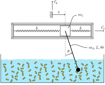
Due to the large demand, your SpaghETH shall increase the production. You decide to automate the blending to the pasta in the water by carefully optimizing its operation. To do that, you start by formulating a model of the system. A sketch is shown in Figure 1.

m₁

m₂, L,Θ x

~e_x

~ey

k k

θ

Figure 1: Sketch of the system.

The blender is modeled as a bar of mass m₂, length L, and moment of inertia (w.r.t.

center of mass) Θ = ₁₂¹m₂L². The blender is attached to a point mass m₁. In order to deal with possible vibrations that might occur in the system, the mass is attached to two springs with spring constant k. Assume the springs are unstretched at x = 0.

Gravitational effects are to be considered; friction and aerodynamic losses are neglected.

1. How many degrees of freedom does the system have? List at least two possible choices of generalized coordinates.

2. Is the system holonomic?

3. Is the system conservative?

4. Determine the kinetic energy of the system.

5. Determine the potential energy of the system.

6. Determine the equations of motion of the system.

7. Describe qualitatively how your answer would change if (a) an external forceF acts horizontally on the mass m₁. (b) the system is brought in an electric field.

Solution.

1. The system has two degrees of freedom. Possible choices of generalized coordinates are (x, θ) and (x, φ), whereφ denotes the angle between the bar the horizontal bar.

Note that (x, x_bar) and (x, y_bar) are not valid choices.

2. Since there are no constraints, the system is holonomic.

3. All forces acting on the system have a potential (or do no work) and therefore the system is conservative.

4. Let ~r₁(t) be the position vector of the mass m and ~r₂(t) the position of the center of mass of the bar. In order to compute the kinetic energy, we first compute the velocities of the mass m and of the bar. In an inertial frame we get

~r₁(t) =



 x 0 0



, ~r₂(t) =





x+^L₂ sin(θ)

−^L₂ cos(θ) 0



.

The velocities are then

~˙ r₁(t) =





˙ x 0 0



, ~r˙₂(t) =





˙

x+ ^L₂θ˙cos(θ)

L

2θ˙sin(θ) 0



.

The angular velocity of the bar is given by

~ ω=



 0 0 θ˙



.

Thus, the kinetic energy of the system is T = 1

2m₁|~r˙₁|²+ 1

2m₂|~r˙₁|²+1 2Θ|~ω|²

= 1

2m₁x˙²+ 1 2m₂

˙ x+ L

2

θ˙cos(θ) 2

+ L² 4

θ˙²sin²(θ)

! + 1

2 1

12m₂L²θ˙²

= 1

2m₁x˙²+ 1 2m₂

˙ x²+L²

4

θ˙²+ ˙xLθ˙cos(θ)

+ 1 2

1

12m₂L²θ˙².

Remark. Alternatively, the velocity of the center of mass of the bar can be computed with

~r˙₂ = ˙~r₁+~ω×~r₁₂ =





˙ x 0 0



+



 0 0 θ˙



×





L 2 sin(θ)

−^L₂ cos(θ) 0



=





˙

x+^L₂θ˙cos(θ)

L

2θ˙sin(θ) 0



.

5. The potential energy of the system is U = 1

2kx²+1

2kx²−m₂gL

2 cos(θ) =kx²−m₂gL

2 cos(θ).

6. The Lagrangian is defined as L=T −V

= 1

2m₁x˙² +1 2m₂

˙

x²+ L² 4

θ˙²+ ˙xLθ˙cos(θ)

+1 2

1

12m₂L²θ˙²−kx²+m₂gL

2 cos(θ).

The derivatives are

∂L

∂x˙ =m₁x˙ +m₂x˙ + 1

2m₂Lθ˙cos(θ),

∂L

∂θ˙ =m₂L² 4

θ˙+1

2m₂Lx˙cos(θ) + 1

12m₂L²θ,˙

∂L

∂x =−2kx,

∂L

∂θ =−1

2m₂xL˙ θ˙sin(θ)−m₂gL

2 sin(θ).

The equation of motion for the generalized coordinate xis d

dt

m₁x˙ +m₂x˙ + 1

2m₂Lθ˙cos(θ)

−(−2kx) = 0

⇒ (m₁+m₂)¨x+ 1 2m₂L

θ¨cos(θ)−θ˙²sin(θ)

+ 2kx= 0.

The equation of motion for the generalized coordinate θ is d

dt

m₂L² 4

θ˙+ 1

2m₂Lx˙cos(θ) + 1

12m₂L²θ˙

−

−1

2m₂xL˙ θ˙sin(θ)−m₂gL 2 sin(θ)

= 0

⇒ m₂ L²

4 +L² 12

θ¨+ 1

2m₂L

¨

xcos(θ)−x˙θ˙sin(θ)

+1

2m₂xL˙ θ˙sin(θ) +m₂gL

2 sin(θ) = 0.

7. (a) The system would not be conservative anymore. The force F has to be con- sidered as generalized force Q₁ acting on the generalized coordinate x. In particular, we have Q₁ =F.

(b) The system is still conservative. The electric potential can be included in U.