Author:LisaSchlüterReviewer:Prof.Dr.SusanneMertensSecondReviewer:Prof.Dr.StefanSchönertSupervisor:Dr.ThierryLasserreJanuary24,2019 EntwicklungneuerMethodenzurBerücksichtigungvonsystematischenEffekteninderAnalysevonerstenTritiumDatenundSensitivitätsstudien

Technical University of Munich

Max Planck Institute for Physics

A thesis submitted in fulfillment of the requirements for the degree of Master of Science

in

Nuclear, Particle and Astrophysics

Development of New Methods to Include Systematic Effects in the First Tritium Data Analysis and Sensitivity Studies

of the KATRIN Experiment

Entwicklung neuer Methoden zur Berücksichtigung von systematischen Effekten

in der Analyse von ersten Tritium Daten und Sensitivitätsstudien im KATRIN Experiment

Author: Lisa Schlüter

Reviewer: Prof. Dr. Susanne Mertens Second Reviewer: Prof. Dr. Stefan Schönert Supervisor: Dr. Thierry Lasserre

January 24, 2019

Erklärung der Selbstständigkeit

Ich versichere hiermit, dass ich die von mir eingereichte Masterarbeit selbstständig verfasst und keine anderen als die angegebenen Quellen und Hilfsmittel benutzt habe.

Declaration of Authorship

I hereby declare that I am the sole author of this master thesis. All direct or indirect sources used are acknowledged as references.

Lisa Schlüter

München, 24.01.2019

Contents

1 Introduction 1

2 Neutrino Physics 3

2.1 Postulation and Discovery . . . . 3

2.2 Neutrino Oscillations . . . . 4

2.3 Neutrino Mass Determination . . . . 7

3 The KATRIN Experiment 11 3.1 Experimental Setup . . . 11

3.2 Model of the Integral Spectrum . . . 15

3.3 Measurement Time Distribution . . . 19

4 Analysis Software and Strategy 21 4.1 Samak . . . 21

4.2 FPD Pixel Combination . . . 22

4.3 Run Combination . . . 23

5 Statistical Methods 29 5.1 Parameter Inference . . . 29

5.2 Confidence Intervals . . . 30

5.3 Uncertainty Propagation . . . 31

5.4 Covariance Matrix Approach . . . 32

5.5 Average of Correlated Parameters . . . 34

6 Assessment of Systematic Uncertainties 37 6.1 General Remarks on Displayed Covariance Matrices . . . 37

6.2 Molecular Final State Distribution . . . 38

6.3 Theoretical Corrections . . . 40

6.4 Tritium Activity Fluctuations . . . 42

6.5 Response Function . . . 42

6.6 Background . . . 44

6.7 Run Combination - Stacking . . . 45

7 First Tritium Campaign 49 7.1 Description of Data . . . 49

7.2 Systematic Uncertainty Budget . . . 51

7.3 Expected Sensitivity . . . 52

7.4 Statistical Analysis . . . 52

7.5 Analysis with Systematic Effects . . . 55

8 KATRIN Neutrino Mass Sensitivity 67

8.1 Elevated Background . . . 67

8.2 Measurement Time Distribution . . . 68

8.3 Systematic Uncertainty Budget . . . 70

8.4 KATRIN Design Report (TDR) Sensitivity . . . 71

8.5 Sensitivity with Current Background Level of 364 mcps . . . 72

8.6 Sensitivity with SDS Background Level of 201 mcps . . . 76

9 Summary and Conclusion 81 Appendices 87 A Measurement Time Distributions 89 B Covariance Matrices 91 B.1 Convergence Test . . . 91

B.2 Final State Distribution . . . 93

B.3 Response Function . . . 94

B.4 Theoretical Corrections . . . 95

C First Tritium Campaign 96

D Neutrino Mass Sensitivity Studies 98

Acknowledgment 105

Chapter 1

Introduction

Neutrinos are the most abundant massive particles in the universe. Their properties, in particular their mass, are central parameters in the fields of particle physics and cosmology. Even though the observation of neutrino oscillations confirmed that neutrinos have non-vanishing mass, they are not sensitive to the absolute mass scale.

However, neutrino oscillations do provide a lower limit of 0.05 eV on the effective mass of the electron antineu- trino m

. Furthermore, the parameter space is limited by an upper bound of 2 eV from direct neutrino mass experiments.

The KArlsruhe TRItium Neurino (KATRIN) experiment is designed measure the effective electron antineutrino mass with an unprecedented sensitivity of 200 meV (90 % C.L.) after five calendar years of data taking. This is achieved in a neutrino mass model-independent way by measuring the tritium β-decay spectrum in the close vicinity of its endpoint at 18.6 keV. Given the tiny fraction of electrons found in this energy region and the minuscule imprint of the neutrino mass on the β-spectrum, the KATRIN experiment is equipped with an ultra-stable windowless high luminosity tritium source and an excellent energy resolution to pursue this ambitious project.

The technique of β-spectroscopy is only sensitive to the squared neutrino mass m

. Therefore, in order to improve the current limit on m

by one order of magnitude, the total uncertainty has to be reduced even by two orders of magnitude with respect to the predecessor experiments. On one hand, the reduction of statistic uncertainty is achieved with a high tritium activity in the source. The suppression of systematic uncertainties, on the other hand, demands a hundredfold higher stability of all experimental parameters, such as the tritium gas density. Remaining systematic effects have to be understood as precisely as possible, mostly below the percent level.

The objective of this thesis is the assessment of systematic uncertainties in the KATRIN experiment with the simu- lation and analysis software Samak, which is largely developed in the framework of this thesis, as working basis.

Various systematic effects are considered, originating from the theoretical tritium spectrum, over the molecular tritium source to the main spectrometer. The associated uncertainties are propagated in a way that they can be applied to both simulation and data using the same technique. For this purpose Samak is equipped with a class, that enables the automatized calculation of covariance matrices for the KATRIN experiment for any desired set of input parameters. The systematic effects are modeled and propagated to the integral spectrum following the philosophy of the MultiSim method. Furthermore features for display, combination of systematic effects and sanity checks, such as a convergence test, are developed. Additionally, a large data base of ready-to-use covariance ma- trices is created. The assessment of systematic effects with covariance matrices allows for the consistent neutrino mass sensitivity estimation on the one hand and the analysis of actual data on the other hand.

The developed treatment of systematic effects is applied in two ways in the course of this work: Firstly, the co-

variance matrices are used in the data analysis of the first KATRIN tritium data, taken in May and June 2018. To

facilitate data handling and to standardize the basic data analyses in Samak, a new tritium data analysis class

is implemented, which allows different run and pixel combination techniques. Through an interface with the

covariance matrix class, the user can choose to include any desired set of systematic effects and their associated

uncertainties in the data analysis. It is demonstrated in this work, that the inclusion of systematic effects yields

a more consistent data analysis in terms of goodness-of-fits and parameter stability over measurement time and

CHAPTER 1. INTRODUCTION

range. Additionally, the impact of different energy loss functions, final state distributions and column densities on the fit results is investigated.

Secondly, a comprehensive neutrino mass sensitivity study is performed in the light of the elevated background

level of the KATRIN experiment. Two timescales are considered: One month of measurement time, which corre-

sponds approximately to the duration of the upcoming first neutrino mass measurement campaign in March 2019,

and the full anticipated measurement period of 30 month. The impact of systematic effects on the sensitivity is

investigated in detail through covariance matrices, calculated individually for every considered set of KATRIN in-

put parameters, such as measurement time distribution or magnetic field strength configuration. Generally, the

higher the background rate, the less pronounced appears the modification of the integral spectrum due to the

neutrino mass. Additionally, the neutrino mass signal is shifted further away from the endpoint with increasing

background levels. From the point of view of statistic uncertainties alone, the loss of neutrino mass sensitivity can

be compensated by exploring larger measurement energy ranges. However, in the frame of this work it is found

that systematic uncertainties increase strongly when extending the measurement interval. Consequently both

statistic and systematic uncertainties have to be taken into account to optimize the measurement time distribution

for upcoming measurement phases.

Chapter 2

Neutrino Physics

Neutrinos are leptons without electric charge. Interacting only weakly, they do not feel the electromagnetic or strong forces, which makes them notoriously difficult to observe. Due to their extremely tiny cross sections, neutrinos are mostly detected indirectly in processes additionally involving charged particles. By measuring the other interaction partners and by applying conservation laws, neutrino properties can be inferred.

There are three sorts of neutrinos, one associated to each lepton family:

 ν

e

‹  ν

µ

‹  ν

τ

‹

. (2.1)

The lepton families differ in their lepton flavors. The electron neutrino ν

is associated with electron flavor, the muon neutrino ν

with the muon flavor and the tau neutrino ν

with the tau flavor respectively. In the current state of knowledge, leptons within a family are connected by lepton number and lepton flavor conversation.

According to these two conservation laws, the number of leptons of a particular family minus the number of the corresponding anti-leptons is conserved within every leptonic interaction. Therefore, the production process in eq. 2.2 is allowed, whereas the one in 2.3 is forbidden. Although neither the lepton number nor the lepton family number conservation comes from any fundamental symmetry in the standard model, the upper limits for their violations are very small [ PRS

15 ] .

π

→ µ

+ ν

(2.2)

π

9 e

+ ν

(2.3)

While masses are assigned to the three charged leptons in the standard model, neutrinos were believed to be massless. However, the discovery of neutrino oscillations in 1998 [ F

98 ] and 2001 [ A

01 ] proved that neutrinos indeed have masses.

This chapter is structured as follows: Section 2.1 gives a brief overview of the postulation and discovery of the neutrino. Thereafter, section 2.2 is devoted to neutrino oscillations and section 2.3 addresses the neutrino mass determination.

2.1 Postulation and Discovery

The joint history of neutrinos and mankind started in the beginning of the 20

century, when radioactivity was first being explored and the nuclear structure was still unraveled. Measurements of β

-decay stirred controversial discussion among physicists: A continuous electron energy spectrum was measured. Believed to be a two-body decay, emitting only a proton and an electron, the energy of the latter should be constant. In an attempt to explain this puzzling observation, Wolfgang Pauli postulated the neutrino in 1930 for the first time in his famous letter to a group of physicists [ Pau30 ] .

Since neutrinos interact only extremely weakly with other particles, it took another 26 years to experimentally

2.2. NEUTRINO OSCILLATIONS CHAPTER 2. NEUTRINO PHYSICS

confirm their existence. In 1956, Cowan and Reines detected within the project poltergeist electron antineutrinos from a nuclear reactor at the Savannah River Site [ CJRH

56 ] . Their detector comprised a liquid scintillator, serving both as target and γ -ray detector, and water doped with cadmium chloride to enhance neutron capture signals. The electron antineutrinos undergo inverse beta decay with the free protons of the liquid scintillator

ν ¯

+ p → e

+ n . (2.4)

The emitted positron annihilates promptly with an electron into two 511 keV photons. After a time delay of several µ s, the neutron is captured by a cadmium nucleus. The capture process releases several γ -rays with a total energy of 9 MeV. This smoking gun signal enabled Cowan and Reines finally to distinguish the electron antineutrinos sig- nal from the immense cosmic backgrounds [ CJRH

56 ] .

2.2 Neutrino Oscillations

2.2.1 Flavor and Mass Eigenstates

The neutrino flavor eigenstates |ν

〉 , |ν

〉 and |ν

〉 are not identical to the neutrino mass eigenstates |ν

〉 , |ν

〉 and

|ν

〉. However, they can be expressed as linear combinations of the mass states





|ν

〉

|ν

〉

|ν

〉



 =





U

U

U

U

U

U

U

U

U









|ν

〉

|ν

〉

|ν

〉



 . (2.5)

The unitary transformation matrix U is called PMNS matrix, named after Pontecorvo, who predicted neutrino- antineutrino oscillations [ Pon58 ] and after Maki, Nakagawa and Sakata, who introduced two flavor neutrino mixing in 1962 [ MNS62 ] . The PMNS matrix contains three mixing angles and three phases. It requires neutrinos to be massive, because the distinction between flavor and mass eigenstates would not make sense otherwise.

Being predicted by the neutrino flavor mixing theory, the observation of neutrino oscillations are a confirmation of this theory and a compelling evidence for neutrino masses.

2.2.2 Two Flavor Oscillation

This section derives neutrino oscillations in the simplified two flavor model. This example illustrates how neutrino oscillations can be observed and additionally, what can learned about the PMNS matrix.

The electron and tau flavor eigenstates can be written as a superposition of two mass eigenstates with only one mixing angle θ

 |ν

〉

|ν

〉

‹

=  cos θ sin θ

− sin θ cos θ

‹  |ν

〉

|ν

〉

‹

. (2.6)

In a weak interaction process, neutrinos are always produced in their flavor eigenstates. Let’s consider an electron neutrino for example:

|ν

〉 = cos θ |ν

〉 + sin θ |ν

〉 . (2.7)

The electron antineutrino carries a fraction of both mass eigenstates. After the interaction, the electron neutrino may propagate freely in space. By applying the time propagation operator e

, the wave function of the physical neutrino |ν〉 after the time t can be written as

|ν( t )〉 = cos θ e

|ν

〉 + sin θ e

|ν

〉. (2.8) The fractions of |ν

〉 and |ν

〉 , carried by |ν〉 , have changed by different magnitudes. This means, that the relative phase of the two mass eigenstates is not constant in time. Therefore, as a particular example the survival proba- bility P

e→νe

, that the neutrino |ν〉 is an electron neutrino is no longer 100 %. Calculated by the modulus square,

CHAPTER 2. NEUTRINO PHYSICS 2.2. NEUTRINO OSCILLATIONS

P

e→νe

is:

P

e→νe

( t ) = || 〈ν( t )|ν

〉 ||

(2.9)

⇒ P

e→νe

( t ) = | cos

θ + sin

θ · e

|

(2.10)

⇒ P

( t ) = 1 − sin

( 2 θ ) sin

 ∆ E t 4

‹

. (2.11)

Neutrino are ultra relativistic particles. Therefore, their energies can be expressed as:

E

= q

p

+ m

= p

v u t 1 + m

p

Taylor

≈ p

+ m

2p

(2.12)

with

p

≈ p ≈ E . (2.13)

It follows, that the survival probability can be rewritten as

⇒ P

e→νe

( t ) = 1 − sin

( 2 θ ) sin

∆ m

L 4E

(2.14) with the neutrino energy E, the traveled distance L and the neutrino mass splitting ∆ m

= m

− m

[ PRS

15 ] . The probability, that the neutrino has a muon flavor, is 1 − P

( t ) respectively.

The oscillation pattern is illustrated in figure 2.1. Starting at the weak interaction point L / E = 0 km / MeV, the electron neutrino has the probability of 1 to have electron flavor. While propagating through space, the survival probability changes. For a 1 MeV electron neutrino it decreases to a minimum of about 0.14 after 15.5 km. The oscillation length, that means the distance between the two maxima is L

≈ 31 km.

By measuring the oscillation pattern, the parameters of the PMNS matrix can be inferred. As can be seen in eq.

2.14, the oscillation amplitude is sensitive to the mixing angle, whereas the neutrino mass splitting can be deduced from the oscillation length.

Figure 2.1: Neutrino oscillation pattern in the two flavor approximation according to eq. 2.14. The mixing angle is assumed to be θ = 34

and the mass splitting ∆ m

= 8 · 10

eV

.

2.2.3 Oscillation Parameters

In order two obtain all neutrino mass splittings and mixing angles, different neutrino sources and various neutrino

energies have to be investigated. Along natural sources like the earth atmosphere, the sun and more distant

2.2. NEUTRINO OSCILLATIONS CHAPTER 2. NEUTRINO PHYSICS

objects in the universe, also man-made sources like particle accelerators and nuclear reactors have been studied in numerous experiments. Although many hints towards the existence of neutrino oscillations were collected before, the Super-Kamiokande experiment and the Sudbury Neutrino Observatory (SNO) finally affirmed their existence.

The Super-Kamiokande experiment observed the oscillation pattern of atmospheric muon neutrinos for the first time, whereas the SNO experiment studied solar neutrinos. This confirmation of neutrino oscillations lead to the award of the Nobel prize to T. Kajita and A. McDonald in 2015. These two measurements and the corresponding oscillation parameters are presented in the following.

Solar neutrino oscillation and the SNO experiment

The Homestake experiment aimed to measure the solar neutrino flux in the 1960s and confronted the physics community with puzzling observation: The measured neutrino flux was too low by a factor of three compared to the flux expected from the solar model [ DHH68 ] . Studying only weak interactions mediated by charged currents, they were solely sensitive to electron neutrinos. Solar muon or tau neutrinos cannot participate in such interac- tions, because their small energies (E < 20 MeV) are insufficient to produce the relatively heavy muons and taus.

However, the solar neutrino problem was resolved in 2001 by the Sudbury Neutrino Observatory (SNO) [ A

01 ] . Additionally measuring neutral current interactions, the SNO experiment was sensitive to all three neutrino fla- vors. They confirmed that electron neutrinos, produced by fusion processes in the sun, change their flavor on their way to earth, while the total number of neutrinos is conserved. The measured neutrino flux is consistent with the solar model.

With neutrino energies in the MeV-range and a large source-detector distance of 1 AU, solar neutrino experiments are especially sensitive to the mixing angle θ

and the mass splitting ∆ m

. They are found to be [ T

]

θ

≈ 34

and ∆ m

≈ 8 · 10

eV

. (2.15)

Atmospheric Neutrinos and the Super-Kamiokande experiment

The earth atmosphere is permanently bombarded with high energetic protons and heavier nuclei from cosmic rays. Interacting with the molecules in the atmosphere, large amounts of pions and kaons are produced, which decay further on into electron neutrinos and muon neutrinos, so called atmospheric neutrinos. The decay results in a flavor ratio of ν

: ν

= 2 : 1 over a wide energy range.

The Kamiokande experiment was the first experiment to observe atmospheric neutrinos. They studied charged current interactions of high energetic electron and muon neutrinos (E > 100 MeV) with ultrapure water in a large underground tank [ PRS

15 ] . Charged leptons, produced in such an interaction, emit Cherenkov light, which is used to reconstruct the directions and energies of the incoming neutrinos. Therefore, they were able to distinguish downgoing neutrinos, flying directly from the atmosphere to the detector and upgoing neutrinos, which traveled a much longer distance through the earth.

The electron neutrino flux neither showed any unexpected angular dependence nor deviated the magnitude from its expectation. Atmospheric neutrinos travel a much shorter distance (20 km-10

km) to the detector than solar neutrinos (1 AU ≈ 1.5 · 10

km). Therefore, the transition ν

→ ν

is not observable on this scale, due to the small mass splitting ∆ m

.

In contrast to that, the muon neutrino flux showed a dependence on the direction of the incident neutrino con- sistent with neutrino oscillations. Additionally, the muon neutrino flux was too low by a factor of two. Since Super-Kamiokande was not sensitive to tau neutrinos, the muon neutrino disappearance was attributed to the transition ν

→ ν

.

The oscillation parameters

were found to be [ T

]

θ

≈ 45

and ∆ m

≈ ∆ m

≈ 2.4 · 10

eV

. (2.16)

1The mixing angleθ13, mentioned for completeness, is in the focus of reactor and accelerator neutrino experiments. It is found to be very smallθ13≈8.3^◦[T⁺].

CHAPTER 2. NEUTRINO PHYSICS 2.3. NEUTRINO MASS DETERMINATION

2.3 Neutrino Mass Determination

Although the neutrino mass splittings ∆ m

can be inferred from neutrino oscillation experiments, the absolute neutrino mass scale is still unknown and cannot be deduced from neutrino oscillations. Currently three methods of neutrino mass determination are being explored, which are briefly presented in the following.

2.3.1 Cosmology

The Λ CDM cosmological model describes the evolution of the universe from the Big Bang to its present state.

Existing in vast abundance, neutrinos have a large influence on structure formation processes in the universe.

Relic neutrinos from the Big Bang still have a number density of 339 neutrinos and antineutrinos per cm

[ LP12 ] . Having a large free streaming length, ultra-relativistic neutrinos act as hot dark matter and wash out small scale structures. Observations of anisotropies in the cosmic microwave background combined with large-scale structures (LSS) provide an upper limit on the sum of neutrino masses

m

= X

i=1

m

. (2.17)

The current bounds lie between 0.12 eV and 0.73 eV [ T

] . However, the determination of the neutrino mass by cosmological observations is rather model dependent. The obtained bounds vary substantially, depending on the underlying data sample, because the model parameters are partly degenerate. That means, that different combinations of parameters can mimic a similar effect. As an example, there is a correlation between the Hubble constant H

and the number of neutrino species [ T

] .

2.3.2 Neutrinoless Double β-Decay

In double β-decays, abbreviated as 2 ν ββ, two neutrons decay weakly into two protons under the emission of two electrons and two electron antineutrinos

2 n → 2 p + 2 e

+ 2 ¯ ν

. (2.18)

Being a second order weak nuclear process, 2 ν ββ may only occur when the single β-decay of a nucleus is en- ergetically forbidden. This is depicted in figure 2.2 (left) for the example of Germanium Ge. The blue parabola represents the mass excess of A = 76 isobars with odd numbers of protons and neutrons, whereas the red parabola stands for the isotopes with even numbers. The smaller the masses of the isotopes are, the larger are their binding energies. The even-even isotopes are shifted towards larger binding energies with respect to the odd-odd isotopes due to the pairing interaction. Being an even-even isotope, Ge would decay in a single β-decay to the isotope with odd numbers Arsenic As, illustrated by the dotted line. However, since the binding energy of As is smaller compared to Ge, this process requires additional energy and is consequently energetically forbidden. Therefore, Ge decays over 2 ν ββ to the even-even isotope Selenium Se. After the first observation in 1987, double β-decay has been measured for 12 different nuclei. The very long half lives are between 10

− 10

y [ GP12 ] .

Neutrinoless double β-decay, abbreviated as 0 ν ββ, is an alternative decay mode, in which the nucleus decays without the emission of neutrinos

2 n → 2 p + 2 e

. (2.19)

It was first proposed by Furry in 1939 [ Fur39 ] following the theory of Majorana, who showed that neutrinos could be their own antiparticles. In this hypothetical interaction, a massive Majorana-type virtual neutrino is exchanged inside the nucleus. However, this process violates lepton number conversation and therefore requires an extension of the standard model. The observation of 0 ν ββ gives access to the absolute scale of the Majorana neutrino mass m

, written in eq. 2.20, because its decay amplitude and therefore the half life depends on the former.

m

= | X

i=1

U

m

| (2.20)

2.3. NEUTRINO MASS DETERMINATION CHAPTER 2. NEUTRINO PHYSICS

This effective electron neutrino mass is the coherent sum over all neutrino mass eigenstates, weighted by the elec- tron neutrino elements of the PMNS matrix. However, due to complex phases in the PMNS matrix, cancellations are possible.

The experimental signature of 0 ν ββ is a monoenergetic peak at the energy of two electrons, shown in figure 2.2 (right). The electrons receive the full decay energy in 0 ν ββ, whereas in 2 ν ββ the decay energy is continuously distributed among the two electrons and two neutrinos. At the present stage, neutrinoless double β-decay has not been observed yet. The current best upper limits on the Majorana neutrino mass comes from the KamLAND-Zen experiment for the Xe isotope [ G

16 ] and from the GERDA experiment for the Ge isotope [ A

18a ] and lie within 61 meV-164 meV (Xe) and 120 meV-260 meV (Ge).

Figure 2.2: Left: Representation of the mass excesses and therefore binding energies of A = 76 isobars. Isotopes with even numbers of protons and neutrons lie on the red parabola, whereas isotopes with odd numbers are located along the blue parabola. The green arrows depict single β-decay. Since the former is energetically forbidden for Ge, this isotope undergoes double β-decay. Adapted from [ GP12 ] . Right: Energy spectra of double β-decay (2 ν ββ) and neutrinoless double β-decay (0 ν ββ). Double β-decay has a continuous energy spectrum, whereas 0 ν ββ manifests itself as a monoenergetic peak. Taken from [ PRS

15 ] .

2.3.3 Single β-Decay

Fermi Theory

During single β

-decay, a neutron decays weakly into a proton while releasing an electron, an electron antineutrino, further on simply referred to as neutrino, and a surplus energy Q

n → p + e

+ ν ¯

+ Q. (2.21)

The surplus energy is distributed among the decay products: The proton receives the recoil energy E

, the neutrino and the electron share the endpoint energy

E

= Q − E

= E

+ E

. (2.22)

Consequently, the energies of electron and neutrino are connected by energy conservation. Even if the neutrino is created without any kinetic energy, the energy available for the electron will differ from the endpoint energy by the rest mass of the neutrino. In more general words: The effective electron antineutrino mass leaves an imprint on the energy spectrum of the β-electron. The effective electron antineutrino mass is defined as the incoherent sum of the three neutrino mass eigenstates

m

= v u t

X

| U

|

· m

. (2.23)

CHAPTER 2. NEUTRINO PHYSICS 2.3. NEUTRINO MASS DETERMINATION

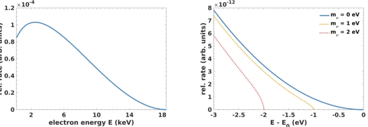
Figure 2.3 (left) depicts the differential energy spectrum of the electron, assuming a neutrino mass of zero. The imprint of m

on the β-spectrum is visualized in figure 2.3 (right) in the close vicinity of the endpoint, where it is most prominent.

The differential spectrum, obtained by the Fermi theory, is given by d Γ

d E = C · F ( Z, E ) · p · ( E + m

) · ( E

− E ) · q

( E

− E )

− m

· Θ( E

− E − m

) (2.24) with the kinetic energy of the electron E and its momentum p. F(Z,E) corresponds to the Fermi function, taking electromagnetic interactions between outgoing electron and daughter nucleus with atomic number Z into account.

The Heavyside function Θ ensures energy conservation. The constant C comprises the Fermi constant G

, the Cabbibo angle θ

and the nuclear matrix element M

[ OW08 ]

C = G

· cos

θ

2 π

· |M

|

. (2.25)

By taking advantage of the neutrino mass imprint on the spectrum, the absolute scale of the neutrino mass can be determined by measuring the β-spectrum. The small magnitude of the neutrino mass signal makes this an extremely difficult venture. The current best upper limit of 2 eV (95 % C.L.) is set by the Mainz [ K

05 ] and Troitsk experiment [ A

11 ] . The KATRIN experiment, described in detail in the following chapter, is the next generation single β-decay experiment.

Figure 2.3: Differential β-spectrum assuming different neutrino mass. The imprint of the neutrino mass is most visible in the close vicinity of the endpoint energy E

.

Theoretical Corrections

Theoretical corrections to the differential β-decay spectrum arise at the particle, nuclear, atomic levels. In addition to the conventional relativistic Fermi function F ( Z, E ) the following effects can be included.

• Radiative corrections: Electromagnetic contributions within the interaction from virtual and real photons.

• Screening: The Coulomb field of the daughter nucleus is screened by the 1s-orbital electrons.

• Recoil effects: Effect of finite nuclear mass in the energy dependent phase space.

• Finite structure of the nucleus: Corrections to Coulomb field of daughter nucleus due to its finite nuclear size and proper convolution of the lepton and nucleonic wave functions through the nuclear volume.

• Recoil of Coulomb field: Correction to Coulomb field, due to non stationary nucleus.

• Orbital-electron interactions: Interchange between the β -particle and the orbital electron.

Further details and the corresponding formulas can be found in [ K

18 ] .

2.3. NEUTRINO MASS DETERMINATION CHAPTER 2. NEUTRINO PHYSICS

Tritium Isotope

The Mainz and Troitsk as well as the KATRIN experiment use tritium to study β-decay. Tritium is a suitable candidate under several aspects [ Mer12 ] .

1. Being a superallowed β

-decay, the decay of tritium has a short lifttime of T

= 12.3 a. This leads to high statistics at rather low source densities.

2. Tritium has the second lowest endpoint E

≈ 18.6 keV of all β-emitters. This leads to an increased relative

count rate close to the endpoint compared to isotopes with higher E

. Additionally, a low endpoint has

technical advantages, because it requires lower voltage of the electrostatic filter, described in 3.1.

Chapter 3

The KATRIN Experiment

The KArlsruhe TRItium Neurino (KATRIN) experiment is the next generation tritium β-decay experiment designed to measure the effective electron antineutrino mass m

to an unprecedented sensitivity of 0.2 eV

(90 % C.L.).

Aiming to improve the sensitivity one order of magnitude with respect to its predecessor experiments in Mainz [ K

05 ] and Troitsk [ A

11 ] , the KATRIN experiment has pushed the established measurement technologies to their limits and is well equipped with a high luminosity tritium source and an excellent energy resolution to pursue this project.

In Section 3.1, an overview of the experimental setup and the working principle of the main components of the KATRIN experiment will be given. Section 3.2 adresses the modeling of the integral tritium β-spectrum. Section 3.3 is devoted to the measurement strategy in the KATRIN experiment.

3.1 Experimental Setup

This section gives a brief overview of the experimental setup of the KATRIN experiment. The particular focus here is on those components, which are essential for the modeling of the integral spectrum, described in 3.2. For a more detailed description of the experimental setup refer to the KATRIN Design Report (TDR) [ A

b ] .

The 70m long setup is depicted in figure 3.1. The tritium β-decay takes place in the windowless gaseous tritium source (WGTS). The β-electrons are further on guided by the transport section to the pre- and main spectrometer, which work as electrostatic high-pass filters. The focal plane detector (FPD) finally counts those electrons, which have energies above a certain threshold.

Figure 3.1: Experimental setup of the KATRIN experiment: a) rear section b) windowless gaseous tritium source (WGTS) c) transport section d1) pre-spectrometer d2) main spectrometer f) focal plane detector (FPD). Figure adapted from [ KAT ] .

1Natural units are used throughout this work: c=ħh=1.

3.1. EXPERIMENTAL SETUP CHAPTER 3. THE KATRIN EXPERIMENT

3.1.1 Rear Section

The rear section is located at one end of the experimental setup. It comprises a gold plated rear wall, which defines the electric potential of the tritium gas in the source. Additionally, it is equipped with calibration and monitoring tools, such as an electron gun [ Sch16 ] .

3.1.2 Windowless Gaseous Tritium Source

Tritium gas is injected through capillaries into the middle of a 10 m long steel tube with a inner diameter of 90 mm, the windowless gaseous tritium source (WGTS). The gas is a mixture of mainly T

, DT, HT and HH. Streaming freely to both ends, the tritium gas molecules are pumped away by different turbomolecular pump stations before being re-injected again. To ensure a very high tritium purity ( > 95 %), the gas is continuously refurbished in this closed tritium loop.

The gas column density ρ d has a design value of 5 · 10

molecules / cm

. The combination of high isotopic purity and column density make the WGTS a high luminosity source with a approximate decay rate of 10

s

. Since variations of the column density are anticipated to be one of the dominant systematic effects, ρ d is targeted to be stabilized at the 10

level.

The source tube is kept at the cryogenic temperature of 27 K. Firstly, this reduces molecular motion and therefore the Doppler-shift of the β-electron energy. Secondly, undesired plasma effects of the source are minimized.

Further on, electrons, which are emitted in forward direction, are guided by superconducting solenoid magnets to the transport section. Electrons, propagating in the opposite direction, are absorbed by the rear wall [ H

17 ] .

3.1.3 Transport Section

The transport section comprises the differential pumping section (DPS) and the cryogenic pumping section (CPS).

The goal of the transport section is to guide the β-electron adiabatically from the source to the spectrometers, while eliminating the tritium flow towards the spectrometer.

The differential pumping section reduces the tritium flow by a factor of 10

with a series of turbomolecular pumps.

The former are not aligned along the beam tube, but tilted by an angle of 20

with respect to each other. This prevents a straight line of sight from the WGTS to the CPS. While β-electrons are magnetically guided along the magnetic field lines through the DPS by five super-conducting magnets, positive ions or molecules are prevented from passing [ L

11 ] .

The cryogenic pumping section reduces the molecular tritium flow by another seven orders of magnitude. Similar to the DPS, the β-electrons are guided adiabatically by seven superconducting magnets. The second and fourth magnet are inclined by an angle of 15

, which leads neutral molecules and positive ions to hit the walls. Here they are absorbed by a 3 K cold cryogenic pump with an argon frost layer [ Rö17 ] .

In total, the transport section reduces the tritium flow by 14 orders of magnitude. This high suppression factor is mandatory to keep the background level in the main spectrometer as low as possible.

3.1.4 Spectrometer Section

The basic idea of the spectrometer section is an integral measurement of the tritium β-spectrum using the estab- lished MAC-E filter principle, which combines the technology of magnetic adiabatic collimation (MAC) with an electrostatic filter (E). The spectrometer section comprises the pre- and main spectrometer, both being MAC-E filters.

Firstly, the general working principle of MAC-E filters is described. Secondly, the two spectrometers in the KATRIN

experiment are presented.

CHAPTER 3. THE KATRIN EXPERIMENT 3.1. EXPERIMENTAL SETUP

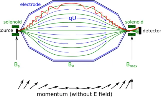
MAC-E Filter Spectroscopy

At both ends of the spectrometer, two solenoid magnets, the source magnet and pinch magnet, produce strong magnetic guiding fields, shown in figure 3.2 by the green lines. Being emitted isotropically in the β -decay, the electrons enter the spectrometer with an acceptance angle of up to 2 π . Due to the Lorentz force, the electrons perform cyclotron motion along the field lines inside the spectrometer, so that their energy is split in a longitudinal and a transversal part with respect to the beam axis:

E

= E

+ E

. (3.1)

A large negative high voltage is applied to the spectrometer vessel forming an electric potential, called retarding potential, depicted in figure 3.2 by the blue arrows, functioning as an electrostatic high-pass filter. Since the di- rection of the electric field is parallel to be magnetic field lines, the electrostatic energy filter is only sensitive to the longitudinal electron energy component. Therefore, only electrons entering the spectrometer with sufficient longitudinal energy pass the electrostatic barrier and are re-accelerated towards the focal plane detector. How- ever, a neutrino mass measurement requires knowledge of the entire energy. This limitation is overcome with the magnetic adiabatic collimation principle, in which the transversal electron energy component is significantly reduced. Technically, this works as follows.

The magnetic field strength B ~ drops towards the center of the spectrometer about four orders of magnitude. The plane inside the spectrometer, in which the minimum of the magnetic field and the maximum of the electric field coincide, is called analyzing plane. The decrease of | B ~ | proceeds slowly along the source side of the spectrometer and the analyzing plane, guaranteeing adiabatic motion of the electrons. As long as the gradient of the magnetic field per electron cyclotron motion is sufficiently small, the magnetic moment µ is conserved:

µ ≈ E

| B ~ | ≈ const. (3.2)

Consequently, the transversal energy component of the electron is slowly transformed into a longitudinal one on the way to the analyzing plane. Because of B

> 0, the energy transformation cannot be perfect and the spectrometer remains insensitive to a residual electron energy fraction ∆ E. It follows from eq. 3.2, that the relative energy resolution of the electrostatic high-pass filter is given by

∆ E E = B

B

. (3.3)

The larger the difference between B

and B

, that means the better the energy resolution, the larger the spectrom- eter has to be to ensure adiabaticity. Having a nominal energy resolution of only 0.93 eV, the main spectrometer requires a length of 23 m.

In addition to the previously described electrostatic reflection, the magnetic field can be used as well to select certain electrons. In case the magnetic field of the pinch magnet at the detector side B

is larger than the magnetic field of the source magnet B

, electrons with emission polar angles larger than θ

are reflected. This effect is called magnetic mirror effect [ A

c ] . The rejection of electrons with large polar angles is advantageous, because these electrons have traveled a longer distance in the source, which enhances the probability of multiple scattering. The maximal polar angle is given by

θ

= arcsin v t B

B

. (3.4)

Pre- and Main Spectrometer

Being located upstream of the main spectrometer, the pre-spectrometer operates at a retarding potential of − 18.3 kV.

Therefore, electrons with energies less than 18.3 keV-18.6 keV = 300 eV below the endpoint are not able to pass

this pre-spectrometer, which is advantageous because they carry no information about the neutrino mass. Addi-

tionally, the electron rate inside the main spectrometer is reduced by seven order of magnitude [ Wan13 ] .

3.1. EXPERIMENTAL SETUP CHAPTER 3. THE KATRIN EXPERIMENT

Figure 3.2: Working principle of the MAC-E filter. The green lines illustrate the magnetic field lines from the source magnetic field B

and pinch magnetic field B

. Moving in cyclotron motions around the magnetic field lines, the electrons are guided through the spectrometer. Only electrons with sufficient energy to overcome the electric retarding potential barrier, here depicted as the blue arrows, are transmitted to the detector. Figure adapted from [ Wan13 ] .

The main spectrometer is located downstream of the pre-spectrometer. Therefore, only electrons with the highest energies are analyzed here. The nominal magnetic field strengths are B

= 3.6 T, B

= 6 T and B

= 3 G, which leads to an excellent energy resolution of 0.93 eV. Table 3.2 gives an overview of the nominal KATRIN settings. To minimize scattering inside the spectrometer, it is operated at ultra-high vacuum of 10

mbar. Additionally, the main spectrometer is equipped with an inner electrode system, consisting of more than 24, 000 wires. In figure 3.2 it is illustrated by the blue lines close to the vessel walls. Set on a lightly more negative electric potential than the spectrometer walls, the inner electrode system blocks muon induced background electrons from the wall [ Are16 ] [ Mer12 ] .

3.1.5 Focal Plane Detector

Electrons, which are transmitted through the main spectrometer, are counted by the focal plane detector (FPD).

These electron are post-accelerated on their way to the FPD to increases the detection efficiency. The FPD is a silicon semiconductor detector, segmented in 148 pixels, as depicted in figure 3.3. Each pixel records its own integral β-spectrum. This allows to correct for slight inhomogeneities of the source, magnetic and electric fields.

The detection efficiency ε

, typically about 0.9, is determined by physical effects such as back-scattering, intrinsic detector properties and by the region of interest (ROI). The ROI defines the energy window, measured by the FPD, within which data is analyzed. Due to the post acceleration towards the FPD of several keV, the ROI thresholds are typically above the tritium endpoint.

Finally, the integral spectrum is measured by counting the transmitted electrons at different retarding potentials.

The measurement strategy in KATRIN is discussed in section 3.3.

CHAPTER 3. THE KATRIN EXPERIMENT 3.2. MODEL OF THE INTEGRAL SPECTRUM

Figure 3.3: The focal plane detector (FPD) is segmented into 148 pixels to correct for inhomogeneities of the source, magnetic and electric fields.

3.2 Model of the Integral Spectrum

This sections is devoted to modeling the integral tritium β-spectrum as it is measured by the KATRIN experiment.

Since tritium is stored in molecular form inside the WGTS, the differential β-spectrum is revised in section 3.2.1.

In section 3.2.2, the response function of the KATRIN experiment is discussed. Finally, all components are joint together into an integral spectrum in section 3.2.3.

3.2.1 Final State Distribution

As described in section 2.3.3, after the β-decay the surplus energy is shared between the kinetic energy of the elec- tron, the total energy of the neutrino, the recoil and excitation energy of the daughter molecule. The so-called final state correction of the differential β-spectrum arises from the varying excitation energy of the daughter molecule.

In its electronic ground state, the excitation energy of the daughter molecule manifests itself in rotational and

vibrational excitations. In addition to that, the electron shells of the daughter molecule have to rearrange them-

selves into the eigenstates of the daughter atomic ion. Therefore, not only the atomic ground state is populated,

but a fraction of the decay ends in states with electronic excitation energy. The first electronic excited state of

the daughter molecule

HeT

has an excitation energy of 27 eV [ SJF ] . The probability distribution, according to

which these excitation energies of the daughter molecule are distributed, is called final state distribution (FSD)

and is illustrated in figure 3.4 for the T

isotopologue. Inside the source, tritium occurs in form of three different

tritiated hydrogen isotopologues, namely T

, DT and HT. To describe the molecular tritium decay in the KATRIN

experiment, the FSD for each isotopologue and its corresponding daughter molecule has to be known. The cor-

rection to the total decay rate

is calculated by summing over all possible final states of each daughter system,

weighted by the respective concentrations in the WGTS.

3.2. MODEL OF THE INTEGRAL SPECTRUM CHAPTER 3. THE KATRIN EXPERIMENT

Figure 3.4: Theoretical calculation of the final state distribution for the T

isotopologue by Saenz et al. [ SJF ] . The leftmost peak corresponds to the rotational and vibrational excitation of daughter molecule (

H eT )

in the electronic ground state. All energies above the first peak, account for the electronic excited final states.

3.2.2 Response Function

The MAC-E transmission function T ( qU, E ) describes the probability, that an electron with the starting energy E is able to pass the main spectrometer at the retarding potential qU:

T ( qU, E ) =



 



 



0 E < qU

1−Ç

1−^E−qU_E ·^Bs_Ba·_γ+1² 1−Ç

1−_Bmax^Bs

qU < E < qU + ∆ E

1 E > qU + ∆ E

(3.5)

The relativistic factor is denoted by γ . It is analytically derivable [ A

b ] . The transmission function is visualized in figure 3.5 (left). Evidently, the transmission probability increases with increasing surplus energy E − qU. Electrons with energies lower than the retarding potential are not able to pass the main spectrometer, while electrons with large surplus energies always overcome the electrostatic potential barrier. However, since not the entire transver- sal electron energy is transformed into longitudinal energy, the MAC-E filter has a nonzero energy resolution.

Electrons with a nonzero starting angle, require a starting angle-dependent amount of surplus energy to make it through the spectrometer. Being averaged over all angles up to θ

, the transmission function in eq. 3.5 only holds for isotropic emission in the source.

The MAC-E transmission function describes only the spectroscopic properties of the MAC-E filter. However, elec- trons may interact along their trajectory from the β-decay in the source to the focal plane detector, losing a fraction of their energy.

Due to the rather high column density ρ d in the WGTS, electrons have a non-negligible probability to scatter inelastically off tritium molecules in the source section. The inelastic scattering probability for an electron with a starting position z inside the WGTS and an emission angle θ to scatter i times is calculated according to [ A

c ] with the inelastic scattering cross section σ

:

P

( z, θ ) = (λ( z, θ ) · σ

)

i! e

. (3.6)

As can be seen in equation 3.6, the scattering probabilities P

( z, θ ) are Poisson distributed. The effective column density λ( z, θ ) , takes the path from the starting point to the exit of the source tube with length L into account:

λ( z, θ) = 1 cos θ

Z

ρ( z

) dz

. (3.7)

CHAPTER 3. THE KATRIN EXPERIMENT 3.2. MODEL OF THE INTEGRAL SPECTRUM

Figure 3.5: Left: KATRIN transmission function for nominal settings. Right: Column density profile inside the WGTS. The effective column density λ integrates the column density over all starting positions z.

Consequently, electrons with a large starting angle or a starting position close to the rear wall have to travel a long way inside the source and are therefore more likely to undergo several inelastic scatterings on their way out.

The column density profile ρ( z

) is depicted in figure 3.5 (right). To obtain the mean scattering probability P

, P

( z, θ ) is integrated over all starting positions and allowed starting angles

P

= 1 ρ d ( 1 − cos θ

)

Z

dz Z

0

d θ sin θρ( z ) P

( z, θ ) . (3.8) Given the nominal ρ d = 5 · 10

molecules / cm

, the probability for an electron to scatter at least once is 59 %.

The scattering probabilities up to ten scatterings for nominal (TDR) KATRIN settings are given in table 3.6.

Electrons also scatter elastically in the WGTS. However, since the elastic scattering cross section is 12 times smaller then the inelastic one, this effect is neglected [ A

b ] .

i 0 1 2 3 4 5 6 7 8 9 10

P

(%) 41.33 29.27 16.73 7.91 3.18 1.11 0.34 0.09 0.02 0.006 0.001 Table 3.1: Mean inelastic scattering probabilities for nominal KATRIN settings.

The energy loss function describes the probability f (") of an electron to loose the energy " during one inelastic scattering. Convolving the function multiple times with itself, the energy loss function for multiple scattering can be determined. This work uses the empirical energy loss function parameterizations from Aseev et al. [ A

c ] and Abdurashitov et al. [ A

a ] . As can be seen in figure 3.6, the parameterizations consist of a Gaussian peak, describing excitation processes, and of a Lorentzian tail, describing the ionization of tritium molecules. The parameterizations employ six parameters, namely the position P and width W of the ionization and excitations peaks as well as the normalization N of the two (eq. 3.9). The parameters describing the excitation part are labeled with index 1, whereas the parameters for the ionization part have index 2. The variable "

is chosen dynamically to ensure the continuity of f (") .

f (") =





 N

exp

− 2

for " ≤ "

N

2 2

W₂²+4("−P₂)²

for " > "

(3.9) The central values of the two parameterizations and their associated uncertainty treatment is discussed in section 6.5. However, the energy loss functions from literature are not precise enough to fit in the tight systematics budget of KATRIN. Therefore, dedicated measurements with a monoenergetic electron gun are scheduled to measure the energy loss function with unprecedented precision.

Finally, the response function R ( E, qU ) , describing both the transmission properties of the main spectrometer as

3.2. MODEL OF THE INTEGRAL SPECTRUM CHAPTER 3. THE KATRIN EXPERIMENT

well as the inelastic scatterings inside the WGTS is calculated by the convolution of the transmission function with the energy loss function:

R ( E, qU ) = Z

0

T ( E − " , qU ) · P

δ(") + P

f (") + P

[ f (") þ f (")] + ...

d " . (3.10) The response function for nominal magnetic fields and column density, is shown in figure 3.7.

Figure 3.6: Energy loss function parametrization from Abdurashitov et al. [ A

a ] for four scatterings.

Figure 3.7: Response function for nominal settings.

3.2.3 Integral Spectrum

Once the response function is calculated, it is straight forward to transform a differential into an integral spectrum:

S ( qU ) = N · Z

qU

d Γ

dE ( E ) · R ( E, qU ) dE + B. (3.11)

CHAPTER 3. THE KATRIN EXPERIMENT 3.3. MEASUREMENT TIME DISTRIBUTION

The normalization factor N accounts for the number of tritium atoms in the source and the maximal starting angle θ

. Additionally, a constant background B is added.

Due to small inhomogeneities in the WGTS and in the electric and magnetic fields in the analyzing plane, every FPD pixels sees a slightly different integral spectrum. In section 4.2, pixel combination techniques are discussed.

Figure 3.8 shows an example of an integral spectrum for nominal settings.

Figure 3.8: Integral spectrum for nominal settings. The nominal settings are given in table 3.2.

parameter value

ρ d 5 · 10

molecules / cm

B

3.6 T

B

6 T

B

3 G

energy resolution ∆ E / E 0.93 eV / 18575 eV

θ

50.77

FPD efficiency 0.9

amount of FPD pixels 148

tritium purity 0.95

T

mol. fraction 0.9

DT mol. fraction 0.05

HT mol. fraction 0.05

background rate 10 mcps

Table 3.2: Nominal settings of main KATRIN parameters. For information on additional parameters refer to [ A

b ] .

3.3 Measurement Time Distribution

As can be seen in eq. 3.11, the integral spectrum is a function of retarding potential qU. The set of qU ~ values, at which the integral spectrum is detected in one measurement, also referred to as one run, is defined by the measurement time distribution (MTD). Additionally, the MTD determines how much time is spent at each retard- ing potential set point, so called subrun. The nominal MTD from the KATRIN Design Report is shown in figure 3.9.

In principle, the MTD could have any arbitrary shape. Aiming for the best neutrino mass sensitivity, most of the

measurement time should be spend in the region of the integral spectrum, in which the neutrino mass imprint is

the strongest. The MTD optimization in the light of higher backgrounds is discussed in section 8.2.

3.3. MEASUREMENT TIME DISTRIBUTION CHAPTER 3. THE KATRIN EXPERIMENT

Figure 3.9: Design Report MTD, optimized for an energy interval of [ E

− 30 eV, E

+ 5 eV ] and nominal KATRIN

settings.

Chapter 4

Analysis Software and Strategy

This chapter is devoted to a brief introduction to the analysis software Samak and the analysis strategy. Section 4.1 addresses the software, which is used throughout this thesis. The analysis strategies, such as pixel and run combination, are presented in sections 4.2 and 4.3.

4.1 Samak

The acronym Samak stands for Simulation and Analysis with MATLAB

for KATRIN. Samak is devoted to analyze tritium β-spectra measured by the KATRIN experiment. For this purpose, Samak contains the following main features:

1. Interface with run summaries

:

To analyze KATRIN data, Samak is able to process the run summaries provided by the KATRIN data taking group. All operational parameters can be retrieved and displayed.

2. Model of tritium β-spectrum:

Integral tritium β-spectra can be modeled according to section 3.2. For data analysis, the model input parameters can be directly read from a run summary. Additionally, Samak is able to generate Monte Carlo data for any desired set of input parameters.

3. Analysis of tritium β-spectrum:

Samak is able to analyze both KATRIN as well as MC data. The main fit parameters in this work are the neutrino mass squared m

, the effective endpoint E

eff

, the signal normalization N and the background B. They are inferred by comparing the data points ~ x to the modeled expectation values for each bin ~µ using a χ

-statistic as described in chapter 5. Additionally, the normalizations of ground state N

and excited states N

within the final state distribution are introduced as two additional fit parameters. Two different minimizers, namely fminuc, a MATLAB

based minimizer, and minuit, a minimizer developed at CERN [ Jam94 ] , are available. Confidence intervals can be constructed, both with statistic and systematic uncertainties with the methods described in section 5.2.

4. Systematic Uncertainties:

Systematic effects are included by covariance matrices as well as with pull terms, described in detail in sections 5.4 and 6. They can be applied both in simulations as well as in the data analysis.

Being written entirely in MATLAB

, Samak is highly vectorized and parallelizable.

1A run summary contains all information about the experiment during one run. Next to the number of counts and theMTD, also slow control parameters such as the column density and the isotopologue concentration is given.