What’s Really the Story with this Balassa-Samuelson Effect in the CEECs? Martin Wagner Jaroslava Hlouskova 04-16 September 2004

Diskussionsschriften

What’s Really the Story with this Balassa-Samuelson Effect in the CEECs?

Martin Wagner Jaroslava Hlouskova

04-16 September 2004

Universität Bern

Volkswirtschaftliches Institut

Gesellschaftstrasse 49

3012 Bern, Switzerland

Tel: 41 (0)31 631 45 06

What’s Really the Story with this Balassa-Samuelson Effect in the CEECs? ^∗

Martin Wagner

University of Bern Department of Economics

Jaroslava Hlouskova

Institute for Advanced Studies Vienna Department of Economics and Finance

September 23, 2004

Abstract

This paper offers a detailed assessment of the Balassa-Samuelson (BS) effect in eight Cen- tral and Eastern European countries (CEEC8). Several features distinguish this study from others: First, we investigate a variety of specifications of extended models. Non- homogeneity of wages, deviations from PPP in tradables and demand side variables are found to importantly contribute to explain inflation differentials. Second, a variety of specifications is investigated. Third, we rely upon bootstrap inference for panel unit root and panel cointegration analysis. The bootstrap results are rather clear: No evidence for cointegration remains when resorting to bootstrap inference. To quantify the bias that may arise from incorrectly using cointegration techniques, we also quantify the BS effect from equations containing (nonstationary) ‘cointegration’ terms. Fourth, we present in- flation simulations based on well specified scenarios.

The results are as follows: Evidence for the BS effect is found. The BS effect is, how- ever, rather small (around half a percent per annum) and not sufficient to explain the observed inflation differentials between the CEEC8 and the EU11. Using, despite the lack- ing evidence, cointegration techniques results throughout in substantially larger estimated effects. This suggests that studies relying upon cointegration may have overestimated the BS effect.

The additional explanatory variables in the extended BS models allow for a satisfactory modelling of the observed inflation rates. The mean inflation simulations for the CEEC8 countries, based on the extended models, range from 2.77% for the Slovak Republic to 6.75% for Poland. These are well above the 2% inflation objective for the European Mon- etary Union.

JEL Classification: F02, O40, O57, P21, P27

Keywords: Balassa-Samuelson effect, Central and Eastern Europe, transition economies, non-stationary panels, bootstrapping, inflation simulations

∗

Financial support from the Jubil¨ aumsfonds of the ¨ Osterreichische Nationalbank under grant Nr. 9557 is gratefully acknowledged. Thanks to M. Kotov for assisting in the data collection and management. We would furthermore like to thank Rumen Dobrinsky for sharing some of his data with us.

†

Corresponding author: Gesellschaftsstrasse 49, CH-3012 Bern, Switzerland; Tel. ++41 31 631 4778, Fax:

++41 31 631 3992, email: martin.wagner@vwi.unibe.ch. Part of this work has been done whilst visiting the

Economics Department of Princeton University, whose hospitality is gratefully acknowledged.

1 Introduction

In this paper we present a detailed econometric study of the Baumol-Bowen (BB) and Balassa- Samuelson (BS) effect for eight Central and Eastern European Countries (CEECs). Studies of these effects have been offered in abundance in recent years. In particular the recent EU enlargement and the subsequent entry of the new member states into the European Monetary Union spur the interest in studies of the real exchange rate and inflation behavior of these economies. Different structural inflation rates across monetary union member states may pose a challenge for common monetary policy, see e.g. Sinn and Reutter (2001). Recent interest in the BS model stems from the fact that it explains differences in inflation rates (respectively real exchange rates) by different productivity growth differentials between the tradables and non-tradables sectors across countries, see the discussion of the model in Section 2. Since larger productivity differentials are often observed in catching-up economies the BS model has been prominent in explaining higher inflation rates in, respectively real exchange rate appreciations of, catching-up economies, see Canozoneri et al. (1999) for OECD country evidence or Mihaljek and Klau (2004) for a study on CEECs.

In our study we try to improve over current practice in the empirical BS literature in several directions. First, the highly stylized theoretical model rests upon a variety of assump- tions that lead to a purely supply side based explanation of real exchange rates respectively inflation rates. We check for the presence of demand side effects and find in particular real per capita GDP important. This finding is consistent with the extension of the BS model pre- sented in Bergstrand (1991). Furthermore we assess in detail the validity of two additional key assumptions of the BS model. These are wage homogeneity across sectors and the prevalence of purchasing power parity (PPP) in tradables. Our econometric analysis leads us to refute both. We thus work with the so called extended versions of the models, that relax these two assumptions. Also, we specify a multitude of equations based on the model. We differentiate the estimation equations along two dimensions. The first is the choice of the dependent vari- able. Since the theoretical model is specified for a two-sector economy, composed of tradables and non-tradables, we use in the narrow specifications only the prices in these two sectors, respectively the real exchange rate with respect to these two sectors as dependent variables.

The broader specifications are less theory driven and use the GDP deflators respectively the

corresponding real exchange rates as dependent variables. The equations with the narrow

dependent variables in general show better fit, as expected. The second dimension along which we distinguish the equations is the choice of the BS variable, see Section 2 for details.

The five choices concerning the BS variable differ e.g. with respect to how sectoral wages are considered. These two specification issues, narrow and wide measure of dependent variables and choices of BS variables, have not yet been treated systematically in the literature.

Second, we acknowledge in our econometric analysis the fact that econometric methods for small nonstationary panels are known to behave unsatisfactorily. Especially panel unit root and panel cointegration tests are known to suffer from severe distortions in small samples, see Hlouskova and Wagner (2004a) or Gutierrez (2003). We try to overcome these limitations by resorting to bootstrapping methods. Various bootstrap algorithms are implemented and lead to similar results: Unit root nonstationarity is found to be widespread amongst the variables. However, essentially no evidence for cointegration is found, when resorting to bootstrap inference. This finding stands in stark contrast with other studies that rely upon panel cointegration methods, see e.g. Egert (2002) or Egert et al. (2002). To assess the bias that is introduced by incorrectly resorting to cointegration techniques, we also quantify the BS effect for well specified equations including error correction terms. We term an equation well specified if all coefficient signs are in line with theory, this includes the coefficient in the

‘cointegrating’ relationship. The results are quite clear for our data for all equations: Using cointegration leads to an over-estimation of the BS effect throughout, partly substantially (by a factor up to four).

We find ample evidence for the BS effect being present. With an average value of about half a percent per annum, it is however too small to explain observed inflation differentials between the CEEC8 and the EU11.

This finding is consistent with the above mentioned observation that several key assumptions of the standard BS model are not supported by the data. Thus, the pure BS effect alone cannot be expected to be too powerful in explaining in- flation differentials, respectively real exchange rate movements. It is the inclusion of variables like deviation from PPP in tradables, relative sectoral wages, real per capita GDP or total consumption that allow for well specified BS type equations with good fit. We therefore base our inflation simulations not just upon the estimated BS effects, but include also the other

1

The ‘foreign country’ used in our study, denoted by EU11, is the aggregate of eleven incumbent EU member

states: Austria, Belgium, Denmark, Finland, France, Germany, Great Britain, Italy, The Netherlands, Spain

and Sweden. The other incumbent EU member states are omitted because of lacking sectoral data. The sample

period for the empirical analysis is 1993–2001 with annual data.

explanatory variables in our inflation simulations, see the details, in particular also concern- ing the scenario assumptions, in Section 7. The bottom line of the large set of results can be roughly summarized as follows: The mean inflation projection is between 2.77% for the Slovak Republic to 6.75% for Poland. The mean prediction for the aggregate inflation of the CEEC8 is 5.43%, with a standard deviation over specifications of about 1.2% inflation rate.

These numbers, are well above the inflation objective of 2% formulated for the European Monetary Union. Also the fact that relatively large inflation differences are predicted across countries, may pose a challenge for monetary policy in an enlarged monetary union.

The paper is organized as follows. In Section 2 we start with a discussion of the theoretical model and the relationships derived thereof for the econometric analysis. Section 3 is devoted to a description of the data and a preliminary graphical investigation of some key elements of the BS model. In Section 4 panel unit root tests are performed and Section 5 is devoted to panel cointegration analysis. In Section 6, based on the results of the previous sections, appropriate equations are specified and the BB and BS effects are quantified. In Section 7 we discuss and present the inflation simulations and Section 8 briefly summarizes and concludes.

Three appendices follow the main text: Appendix A contains a detailed description of the data, their sources and preliminary variable transformations. In Appendix B a multitude of additional empirical results is collected and in Appendix C the implemented bootstrap algorithms are briefly described.

2 The Baumol-Bowen and the Balassa-Samuelson Effect

Balassa (1964) and Samuelson (1964) present models in which different productivity growth differentials between the tradables and non-tradables goods sectors across countries are an important factor in explaining real exchange rate movements, respectively differences in the evolution of national price levels.

The model is formulated in terms of a two-sector small open economy. The small open economy assumption implies that the world interest rate R and the world market price of tradables P

are taken as given. Both sectors, tradables (T) and non-tradables (N), are described by their sectoral production functions, which are for algebraic simplicity assumed

2

Recently Ghironi and Melitz (2003) presented a very interesting stochastic general equilibrium model with

heterogeneous firms that leads to BS type effects. An econometric analysis of that model will be an interesting

challenge for the BS community. An earlier general equilibrium analysis of the BS model is given by Asea and

Mendoza (1994).

to be Cobb-Douglas:

Y

= A

(K

)

(L

)

Y

= A

(K

)

(L

)

(1) where Y

, with s ∈ { T, N } , denotes real output in sector s; A

, K

and L

denote (total factor) productivity, capital and labor in the respective sector; and α

denotes labor intensity in each sector. The productivities and the labor intensities are allowed to differ across the two sectors. Both sectors are assumed to be composed of perfectly competitive firms and production factors are assumed to be fully utilized. The assumptions imply that only the supply side of the economy influences the evolution of the real exchange rate. The potential effect of demand side factors for the evolution of the real exchange rate in the CEECs is tested in Section 6.

The assumption of perfect competition in both sectors leads to the following first order conditions for profit maximization, with W

and W

denoting the wages in the tradables and non-tradables sector.

R = (1 − α

)A

K^T

= P

(1 − α

)A

K^N

W

= α

A

W

= P

α

A

(2)

where P

= P

/P

denotes the relative price of non-tradables.

Concerning the labor market, in the standard Balassa-Samuelson model perfect labor mobility across the two sectors is assumed. This results in wage homogeneity, W

= W

. Under this additional assumption the above equations can be solved to obtain the following expression for the logarithm of relative prices.

p

= c + α

α

a

− a

(3)

where c is a constant depending upon the exogenously given factor intensities (α

, α

) and the interest rate. Throughout the letter c is used to denote constants in the various equations, those are not necessarily the same across equations. The above equation (3) displays the

3

The choice of Cobb-Douglas functions, with its algebraic convenience of leading to simple log-linear equi- librium relationships, is of course an approximation. Thus, some flexibility in the empirical modelling might be required.

4

Throughout the discussion we consider the tradables good as the numeraire.

5

Lower case letters indicate logarithms of variables throughout.

link between the relative prices in the two sectors and, up to the factor

, the relative productivities. This effect is known in the literature as the Baumol-Bowen effect, see Baumol and Bowen (1966). The underlying logic of the argument is simple: For simplicity of the verbal argument assume for the moment that α

= α

. Assume further that productivity growth is faster in the tradables sector than in the non-tradables sector, i.e. ∆a

> ∆a

. Now, if productivity grows faster in the tradables sector, this allows for wages to grow faster in this sector (given the exogenous world market prices for tradables and capital). Due to the assumed labor mobility, the non-tradables sector has to pay the same wages as the tradables sector. This implies, due to lower productivity growth, that the non-tradables sector has to raise its prices (faster) in order to remain profitable. Thus, higher productivity growth in the tradables sector leads to higher inflation in the non-tradables sector. Note that in many countries the labor intensity is higher in the non-tradables sector than in the tradables sector, i.e. α

> α

, which reinforces the above argument where we assumed identical intensities for simplicity.

Surprisingly, many empirical studies like Alberola and Tyrv¨ ainen (1998), Coricelli and Jazbec (2004a), Coricelli and Jazbec (2004b), Halpern and Wyplosz (2002) or Sinn and Reut- ter (2001) that claim to study the Balassa-Samuelson effect are in fact studying the Baumol- Bowen effect. The imprecision in the distinction may stem from the fact that the relative price of non-tradables to tradables is often used as an internal measure for the real exchange rate. This measure, however, will in general differ substantially from other real exchange rate variables, based on the GDP or CPI deflators or also the trade weighted real exchange rate.

Note also that the Baumol-Bowen effect is only concerned with domestic variables, thus in particular it cannot explain any inflation differentials across countries. The Baumol-Bowen effect is only one important part of the Balassa-Samuelson effect, as will become clear below.

Without the assumption of sectoral labor mobility and the implied wage homogeneity, the above equation (3) is modified to

p

= c + α

α

a

− a

+ α

(w

− w

) (4) The interpretation of this extended Baumol-Bowen effect is similar to the explanation given above. Now, for example, lower wage growth in the non-tradables sector can mitigate the relative inflation pressure.

The Balassa-Samuelson effect itself combines the above domestic Baumol-Bowen effect

with the (evolution of the) real exchange rate. Starred variables henceforth denote the foreign country, or the rest of the world. In our empirical analysis the foreign country is given by, as already stated, the EU11. The real exchange rate for a country is defined as Q =

, where E denotes the nominal exchange rate (local currency per Euro) and P and P

denote the domestic and foreign aggregate price levels. Throughout the paper variables for the EU11 are indicated with a ‘*’. The aggregate price levels are weighted averages (weighted by expenditure shares δ) of the sectoral price levels, i.e. in logarithms they are given by:

p = (1 − δ)p

+ δp

p

= (1 − δ

)p

+ δ

p

(5) Combining the above price level decompositions with the definition of the real exchange rate directly leads to

q = (e + p

− p

) − δ(p

− p

) + δ

(p

− p

) (6) Thus, the (logarithm of the) real exchange rate is seen to depend upon three factors: The first is the real exchange rate in the tradables sector. It is commonly assumed that PPP holds in the tradables sector, this implies e + p

− p

= 0. Thus, under this assumption the first term vanishes. The second and third term are the relative prices of non-tradables in both countries, weighted by their shares in the overall price level. Inserting the expressions for the relative prices found above, leads to the Balassa-Samuelson model, that explains the real exchange rate in terms of productivity differentials at home and abroad

q = c + (e + p

− p

) − δ

α

α

a

− a

+ δ

α

α

a

− a

(7) Given that PPP holds in the tradables sector, the real exchange rate is given by:

q = c − δ α

α

a

− a

+ δ

α

α

a

− a

(8) The above equation (8) implies, for sufficiently similar labor intensities and expenditure shares, that the real exchange rate of the country appreciates (∆q < 0), if its sectoral pro- ductivity growth rate differential is larger than the productivity growth differential abroad.

The fact that this differential is often found to be bigger in faster growing or catching-up

economies, makes the Balassa-Samuelson model a widely used model for explaining real ex-

change rate appreciations. Employing once again the definition of the real exchange rate, the

above equation (8) can be modified and differenced to describe inflation differentials across

countries:

∆p − ∆p

= c + ∆e + δ α

α

∆a

− ∆a

− δ

α

α

∆a

− ∆a

(9) The inflation differential depends upon nominal exchange rate movements and the differences in the sectoral productivity growth differentials across countries. In a monetary union, the nominal exchange rate is by construction fixed, and inflation differentials are, according to the model, solely determined by productivity growth differentials across member states of a monetary union.

As for the Baumol-Bowen effect discussed above, also for the Balassa-Samuelson effect the assumption of wage homogeneity across sectors can be relaxed. This results in the following generalization of equation (9), now again in levels:

p − p

= c + e + δ

α^T

a

− a

+ α

(w

− w

)

− δ

α^T∗

a

− a

+ α

(w

− w

)

(10)

Abstaining from the assumption of PPP for traded goods, we obtain the following reformu- lation of equation (9)

∆p − ∆p

= c + ∆p

− ∆p

+ δ α

α

∆a

− ∆a

− δ

α

α

∆a

− ∆a

(11) which holds without any assumption on the nominal exchange rate. Now inflation differen- tials depend upon tradables inflation differentials and the differences in productivity growth differentials. Of course, as above, also the extension allowing for non-homogenous wages can (and will) be investigated:

∆p − ∆p

= c + ∆p

− ∆p

+ δ

α^T

∆a

− ∆a

+ α

(w

− w

)

−

δ

α^T∗

∆a

− ∆a

+ α

(w

− w

)

(12)

From the above relationships various variables that correspond to the Balassa-Samuelson effect can be derived. The variable BS

= δ

a

− δ

a

follows from equation (8) after setting α

= α

in both the CEE country and the EU11, with a

= a

− a

.

Here and throughout the paper in the double sub-script it, i is the country and t the time index.

These are dropped when unnecessary. The shares δ

can be easily computed by δ

=

Y_it^T+Y_it^N

. Taking into account the non-homogeneity of wages (established below), the variable BSE1

is

6

We furthermore experimented with variables that contain

α^T

a

− a

instead of a

− a

. These variables,

despite their theoretical appeal do not lead to satisfactory econometric analysis and results. This may inter

alia reflect that the sectoral production functions are not exactly Cobb-Douglas.

computed as follows BSE 1

= δ

(a

+α

w

) − δ

(a

+α

w

), with w

= w

− w

. Implicitly setting δ

= δ

, i.e. ignoring differences in the sectoral composition across the CEE countries and the EU11, defines the variable BSE2

= (a

+ α

w

) − (a

+ α

w

).

Finally also the differential of relative productivities, a

− a

, is used as a BS variable.

This latter choice is probably the most widely used variable, despite or because of neglecting some Cobb-Douglas related constants.

As indicated in the introduction in the following sections the above relationships are investigated using panel unit root and panel cointegration techniques. Usage of this type of techniques rests upon the first tested assumption of unit-root non-stationarity for the macro- variables used. Unit-root non-stationarity combined with the presence of cointegration as laid out by the above relationships leads to error-correction models for the evolution of the (rate of appreciation of the) real exchange rate, respectively of the inflation differentials. In the empirical analysis we furthermore address the potential impact of demand side factors on the evolution of prices and exchange rates.

3 Data and Preliminary Investigations

The study is conducted for eight Central and Eastern European countries (CEEC8): the Czech Republic (CZE), Estonia (EST), Hungary (HUN), Latvia (LVA), Lithuania (LTU), Poland (POL), the Slovak Republic (SVK) and Slovenia (SVN). The foreign country in the empirical study is, as mentioned, comprised by the aggregate of eleven incumbent EU (EU11) member states, these are the EU15 excluding Greece, Ireland, Luxembourg and Portugal.

These four countries are omitted because of incomplete data. Note, however, that these are all relatively small economies that are rather unrelated to our CEE countries. Thus, the effect of the omission of these countries in the construction of the foreign country can be expected to be modest. The data are annual and the sample period is 1993–2001. This is also the sample period used throughout the econometrics in the subsequent sections.

The first decision to make is, of course, the sectoral classification. We decide to take

NACE sectors C (mining and quarrying), D (manufacturing) and E (electricity, gas and

water supply) as our tradables (T) sector. Non-tradables (N) is composed of NACE sectors

F (construction) to K (real estate and business activities). NACE sectors A and B are

aggregated to agriculture (AGR) and sectors L to P are aggregated to the public sector

(PUB). See Table 20 in Appendix A for details.

A description of all available variables and their sources is given in Tables 21 and 22. For reference purposes all variable transformations prior to econometric analysis are collected in Table 23. The precise construction of the EU11 aggregates for the tradable and the non- tradable sectors is contained in Table 24. These are aggregated using sectoral output weights.

All these tables describing the data and preliminary variable transformations are contained in Appendix A.

With the chosen classification, about 70 to 80 % of the economy are taken into account, see the right block of Table 1. The two neglected sectors, agriculture and the public sector, have quite substantial inflation rates, see columns five and six of Table 1. For this reason, we have decided to specify the empirical analogues of equations (7) to (12), derived in the previous section, with two different price indices respectively two different real exchange rate measures.

The two price differentials are given by p

− p

, i.e. the difference in the (logarithms of the) GDP deflators. Following Harberger (2004) and based on the fact that our model is specifying the supply side of the economy, we have decided to use the GDP deflator as our broad price measure. The other possible choice for a broader price aggregate would be the consumer price index (CPI). The correlation between the GDP based inflation rates and the HICP (Harmonized Index of Consumer Prices) inflation rates is close to one for most countries. Thus, no qualitative differences in the results have to be expected.

The second price differential chosen is given by p

− p

, i.e. by the differential of the log price levels only in the two sectors tradables and non-tradables. Similarly to the two price variables also the corresponding two real exchange rate measures have been chosen, q

= e

+ p

− p

and q

= e

+ p

− p

. From the definition of the variables it immediately follows that the predictions concerning the coefficient signs in the p-equations are opposite those for the q-equations. Specifying two sets of equations, based on a narrow and a wide price respectively real exchange rate measure, allows us to assess the effect of the choice of dependent variable on the results. This is an issue up to now entirely neglected in the empirical literature. In the sequel we denote with p-equations the equations with the two price (differentials) as dependent variables and with q-equations the equations

7

The empirical specifications will partly include further explanatory variables. All equations include relative wage terms and terms related to the real exchange rate of tradables. See the discussion below.

8

The correlation between GDP deflator and HICP inflation rates over the period 1994–2001 is e.g. 0.95 for

Sweden or 0.86 for the Netherlands. The average correlation across the EU11 is 0.81. For only two countries

is the correlation below 0.7, Belgium and Finland. Not only the correlation between the HICP and the GDP

deflator inflation is very high, also the dynamics of the two variables are very similar for all countries.

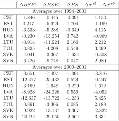
Sectoral shares in total output

Country ∆a

∆a

∆p

∆p

∆p

∆p

T N AGR PUB

Averages over 1994–2001

CZE 5.15 2.17 5.14 6.51 6.39 12.06 0.35 0.47 0.05 0.13

EST 6.38 5.72 12.53 14.27 11.68 18.43 0.24 0.50 0.08 0.18 HUN 6.87 0.92 11.77 15.70 11.68 15.01 0.28 0.46 0.06 0.20

LVA 6.92 6.06 6.01 10.94 4.38 17.08 0.28 0.47 0.09 0.17

LTU 6.07 2.02 12.84 14.78 8.71 23.52 0.26 0.47 0.12 0.15 POL 7.99 2.66 7.93 18.61 12.36 17.03 0.33 0.45 0.06 0.16

SVK 3.82 2.30 5.86 8.03 5.31 6.33 0.31 0.47 0.06 0.16

SVN 6.96 2.15 9.47 12.31 8.92 11.11 0.33 0.44 0.04 0.20

EU11 2.84 1.01 1.25 2.03 0.70 2.82 0.24 0.53 0.02 0.21

Averages over 2000–2001

CZE 5.6 7.9 2.2 0.9 9.1 7.8 0.35 0.49 0.05 0.11

EST 8.4 7.1 5.3 5.5 8.1 4.1 0.24 0.52 0.06 0.17

HUN 4.8 1.6 7.4 9.5 6.7 10.9 0.31 0.45 0.05 0.19

LVA 4.8 7.3 1.2 3.1 7.4 6.5 0.26 0.50 0.08 0.16

LTU 12.7 5.8 5.5 1.3 -1.7 0.8 0.27 0.48 0.11 0.15

POL 6.8 3.1 1.3 8.0 14.0 16.1 0.34 0.46 0.05 0.15

SVK 0.3 1.6 4.2 7.6 9.5 0.0 0.31 0.47 0.05 0.17

SVN 6.6 1.7 6.4 11.8 9.3 11.2 0.33 0.43 0.04 0.20

EU11 2.3 0.8 1.8 2.2 3.2 3.2 0.23 0.54 0.02 0.21

Table 1: Sectoral productivity growth rates, sectoral inflation rates and sectoral output shares.

The top panel displays the average annual growth rates over the period 1994–2001 and the lower panel over the period 2000–2001.

that have the real exchange rate measures as dependent variables.

In Table 1 we also display the average sectoral productivity growth rates in the tradables and non-tradables sectors. Consider the productivity growth rates first. For the larger period, displayed in the top panel, it holds in all CEECs and the EU11 that productivity grows faster in the tradables sector than in the non-tradables sector. For the shorter period 2000–2001 this does not hold for the Czech Republic, Latvia and the Slovak Republic. Also note that the differentials vary substantially across countries. For example in the Slovak Republic the productivity growth differential (over the period 1994–2001) is smaller (1.52%) than in the EU11 (1.83%). Thus, we can already expect substantial differences across countries, concerning the extent of dual inflation pressures via sectoral productivity differentials.

Concerning sectoral inflation rates, we see in columns three and four that (again for the longer period) the non-tradables sector has a higher inflation rate than the tradables sector.

For the shorter period again some opposite inflation dynamics occur, in the Czech Republic

and in Lithuania.

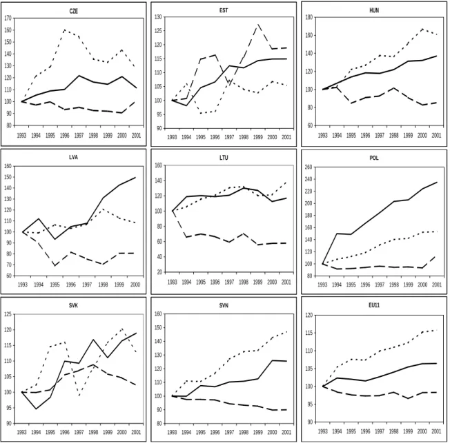
Summing up the information from Table 1, some key facts in line with the Baumol- Bowen model are present in the data for the CEECs: Higher productivity growth rates in the tradables sector and higher inflation rates in the non-tradables sector. In Figure 1 roughly the same information is also shown graphically. For all countries and the EU11 we display, over the period 1993–2001 in solid lines the relative price of non-tradables to tradables, in fine dashed lines the relative productivity of tradables to non-tradables and in dashed lines the relative wages in the non-tradables sector relative to wages in the tradables sector. Thus, the relative prices and relative productivities are displayed in such a way that they should grow over time, if behaving according to the model with higher productivity growth in tradables and higher inflation in non-tradables. Wage homogeneity across sectors implies that the relative wages should not exhibit trending behavior. The evidence is mixed. Concerning relative wages we observe stable relative wages in the Czech Republic, Poland, Slovenia and the EU11, in other countries wage homogeneity seems to be violated.

Relative prices and productivities exhibit co-movements, with differing degrees of synchronicity. E.g. in Lithuania there is an almost one-to-one relation between relative prices and productivities.

Table 1 and Figure 1 allow for a first graphical assessment of the prevalence of a Baumol- Bowen effect in the CEECs. In the following Figure 2 we take a first look at a potential Balassa-Samuelson effect in the CEECs with respect to the EU11. The figure displays for three different periods the differential of the relative productivity growth rates in the CEECs,

∆a

, to the relative productivity growth rate in the EU11, ∆a

against the inflation rate differential between the CEEC countries, ∆p

and the EU11, ∆p

.

In its standard version, the Balassa-Samuelson effect implies a positive correlation between sectoral productivity growth differentials and inflation differentials, compare e.g. equation (9). This is supported by Figure 2. The correlations are 0.458 for the longest period 1994–2001, 0.836 for the period 1996–2001 and 0.419 for the shorter period 2000–2001. We already know from the above discussion that over the period 2000–2001 in several countries behavior not supporting the standard BS setup has been observed. This translates into the lower correlation over that short period. One further important observation can be made in the figure. For three or

9

Formal econometric tests for wage homogeneity will be presented in the following sections, in the context of panel unit root and panel cointegration analysis. The tests reject the null hypothesis of wage homogeneity in the panel of eight CEE countries.

10

Note that the inflation rates are only computed for the tradables and non-tradables sectors. Similar

pictures with the GDP deflators exhibit also positive correlation, albeit slightly less pronounced.

CZE

80 90 100 110 120 130 140 150 160 170

1993 1994 1995 1996 1997 1998 1999 2000 2001

EST

90 95 100 105 110 115 120 125 130

1993 1994 1995 1996 1997 1998 1999 2000 2001

HUN

60 80 100 120 140 160 180

1993 1994 1995 1996 1997 1998 1999 2000 2001

LVA

60 70 80 90 100 110 120 130 140 150 160

1993 1994 1995 1996 1997 1998 1999 2000

LTU

20 40 60 80 100 120 140 160

1993 1994 1995 1996 1997 1998 1999 2000 2001

POL

80 100 120 140 160 180 200 220 240 260

1993 1994 1995 1996 1997 1998 1999 2000 2001

SVK

90 95 100 105 110 115 120 125

1993 1994 1995 1996 1997 1998 1999 2000 2001

SVN

80 90 100 110 120 130 140 150 160

1993 1994 1995 1996 1997 1998 1999 2000 2001

EU11

90 95 100 105 110 115 120

1993 1994 1995 1996 1997 1998 1999 2000 2001

Figure 1: Solid lines: relative prices of non-tradables to tradables (N/T); fine dashed lines:

relative productivities in tradables and non-tradables sector (T/N); dashed lines: relative

wages in non-tradables and tradables sector (N/T). All quantities normalized to 100 in 1993.

1994-2001

0 2 4 6 8 10 12 14

-2 -1 0 1 2 3 4 5

d(a^rel)-d(a^rel*)

d(pT+N)-d(pT+N*)

EST

LVA

SVK CZE LTU POL

SVN HUN

1996-2001

0 2 4 6 8 10 12

-2 -1 0 1 2 3 4 5

d(a^rel)-d(a^rel*)

d(pT+N)-d(pT+N*)

CZE SVK LVA

LTU

EST POL

HUN

SVN

2000-2001

-2 -1 0 1 2 3 4 5 6 7 8

-8 -6 -4 -2 0 2 4 6 8

d(a^rel)-d(a^rel*)

d(pT+N)-d(pT+N*)

LVA

CZE SVK

EST HUN

POL SVN

LTU

Figure 2: Relative productivity (T/N) and inflation differentials to the EU11. The inflation rates are computed only over the tradables and non-tradables sectors. The left chart displays the averages over the period 1994–2001, the chart in the middle displays the averages over the period 1996–2001 and the right chart over the period 2000–2001.

four out of eight countries, depending upon the period, the relative productivity differential growth rate is smaller than in the EU11. Thus, for these countries and these periods the standard BS model actually implies smaller inflation in the CEE countries than in the EU11.

Combining this with the observed higher inflation rate in all CEE countries compared to the EU11 directly implies that the contribution of the BS term, which ever way measured, to inflation will be limited, despite the positive unconditional correlation. The model thus needs to be augmented by further explanatory variables, like the extensions discussed in Section 2 or demand side variables discussed as below in Section 6.

The evidence gained in this section by considering averages and also by graphical inspec- tion of some key ratios and relationships is grosso modo sufficiently positive to turn to formal econometric analysis. The non-stationary character of many of the series requires us to first establish unit root type non-stationarity in order to be able to use (panel) cointegration anal- ysis to test for ‘long-run’ relationships. We turn to both of these issues in the subsequent two sections.

4 Econometric Analysis I: Panel Unit Root Testing

The small sample size with only nine years necessitates the application of panel unit root tests. The implemented panel unit root tests are developed in the following papers:

Levin,

11

As indicated already above, the implementation of the econometric procedures was originally based on

Chiang and Kao (2002), but has been substantially modified, corrected and extended. The authors currently

Lin and Chu (2002), abbreviated by LL; Breitung (2000), abbreviated by U B; two tests developed in Im, Pesaran and Shin (1997) and Im, Pesaran and Shin (2003), a t-type test abbreviated by IP S and a Lagrange multiplier test, abbreviated by IP S − LM ; Harris and Tzavalis (1999), abbreviated by HT ; and Maddala and Wu (1999), abbreviated by M W .

All tests except for HT allow for individual specific serial correlation structures, whilst HT is designed for the case of no serial correlation in the residuals. For all tests the null hypothesis is that of a unit root in all series. The alternative is stationarity in all series, except for the tests developed by Im et al. where the alternative allows for non-stationarity in a non- vanishing (in the limit for N → ∞ ) fraction of the series. The first five tests listed above are asymptotically normally distributed and the latter is asymptotically χ

distributed, with N denoting the cross section dimension of the panel. The test LL, U B, IP S and HT are left-sided and IP S − LM and M W are right sided.

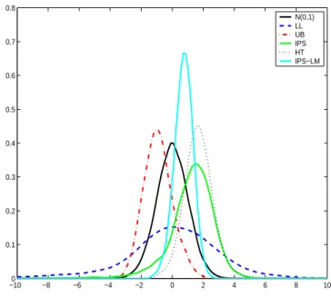
It has been found, see e.g. Hlouskova and Wagner (2004a,b), that for panels of the size available in this study, the asymptotic distributions of the panel unit root and panel cointegration tests provide poor approximations to the small sample distributions (for an example see Figure 3 and the corresponding discussion below). In other words, the notorious size and power problems for which unit root tests are known in the time series context also appear in small or short panels.

To overcome these limitations we have implemented three different bootstrap methods to obtain improved small sample inference. The three bootstrap methods, explained in Ap- pendix C, are the parametric, the non-parametric and the residual based block bootstrap. The latter has been developed for non-stationary time series by Paparoditis and Politis (2003).

The former two methods obtain white noise bootstrap replications of residuals due to pre- whitening and the latter is based on re-sampling blocks of residuals to preserve the serial correlation structure. The difference between the parametric and the non-parametric boot- strap is essentially given by the fact that in the former the residuals are drawn from a normal distribution and are re-sampled from the empirical residuals in the latter. The results ob- tained by the three bootstrap methods are rather similar, thus in the main text we only report the result from one of the methods. Note furthermore that bootstrapping, if re-sampling is done identically for all cross-sectional units, also provides certain robustness against the vio-

work on a user friendly version of the new toolbox. A detailed description of these panel unit root tests,

including the assumptions on the data generating process and the precise construction of the test statistics, is

given e.g. in Hlouskova and Wagner (2004a).

−100 −8 −6 −4 −2 0 2 4 6 8 10 0.1

0.2 0.3 0.4 0.5 0.6 0.7 0.8

N(0,1) LL UB IPS HT IPS−LM

Figure 3: Bootstrap test statistic distributions for relative prices, p

, for the five asymptot- ically standard normally distributed panel unit root tests.

The results are based on the non-parametric bootstrap with 5000 replications. Fixed effects are included.

lation of a key assumption of all the implemented unit root tests, namely the assumption of cross-sectional independence, see e.g. Chang (2000). In Figure 3 we display the asymptotic null distribution (the standard normal distribution) and the bootstrap null distributions (from the non-parametric bootstrap) for one of the variables tested for a unit root, the relative price of non-tradables to tradables, p

, for the five asymptotically standard normally distributed tests. The figure shows substantial differences between the bootstrap approximations to the finite sample distribution of the tests and their asymptotic distribution. Thus, basing infer- ence on the asymptotic critical values leads to substantial size distortions. This can also be seen in Tables 2 and 3 below, where in brackets the bootstrap 5% critical values are displayed.

They vary substantially both across tests and also across variables, and are in many cases far away from the asymptotic critical values ± 1.645, respectively 26.296 for the Maddala and Wu test.

All tests are implemented, as is standard in the unit root literature, with different speci-

fications of the deterministic terms. We have tested with two versions, for each of the three

bootstrap algorithms. With fixed effects only, reported in Table 2 and with fixed effects and

individual specific linear trends, reported in Table 3. These tables report the results based on

the parametric bootstrap. All bootstrap results in this paper are based on 5000 replications.

Including a linear trend in the test equation, when there is no trend in the data generating process reduces the power of the tests, on the other hand, omitting a linear trend when there is a trend in the data, induces a bias in the tests towards the null hypothesis. Graphical inspection of the data shows that for basically all variables, even the relative price or wage variables, in at least one or two countries trending behavior is visible. This implies that in the panel framework the specification with trends may be more appropriate. As is common in the unit root literature, we however present and compare the results of both specifications for all variables. The comparison of the results obtained with different specifications is usually informative.

The variables for which we report the panel unit root test results are the following.

Three real exchange rate measures, q the logarithm of the real exchange of the CEEC countries to the EU11 (indexed to equal 100 in 1995) based on the GDP deflators; q

defined similarly to q but based on the price indices of only the tradables and non-tradables sectors; and q

, the real exchange rate for tradables (again in logarithms and indexed). The latter is directly related to one of the assumptions of the standard Baumol-Bowen and Balassa-Samuelson models, namely prevalence of PPP in the tradables sector. The econometric testing for validity of PPP in a world of I(1) nonstationary data is to test for stationarity of the real exchange rate. This, of course, allows for substantial and persistent differences in prices. The unit root hypothesis is hardly at all rejected for these variables, in particular if one relies on bootstrap based inference, then only for q

two tests reject the null when a trend is included.

In particular also note that for q

some rejections occur based on the asymptotic critical values, but no rejection occurs based on the bootstrap critical values. Thus, we conclude that PPP does not hold in the tradables sector between the CEE countries and the EU11.

The second group of variables tested are the various (logarithms of) price variables. The relative price of non-tradables to tradables and different price level differentials between the CEE countries and the EU11. For the price level differentials it is not a priori clear which specification is preferable, since due to catching-up of the CEE countries persistent inflation differentials and thus a narrowing of price differentials might induce a trend in the price level

12

See also Table 23 for a summary description of the variables and transformations. Note that also for the

output variables and the prices the null hypothesis of a unit root can generally not be rejected, detailed results

are available from the authors upon request. In the presentation here we focus on those variables and their

relationships that are directly relevant for the model only.

differences.

Concerning the relative price, p

, the hypothesis of a unit root is never rejected in both specifications. For the price level differentials the evidence is a bit more mixed. The tests IP S and M W reject, based on the bootstrap critical values, the null of a unit root for all three price level differentials, p

− p

, p

− p

and p

− p

. Also IP S − LM is rejecting the null for these three variables. When a linear trend is included in the test equation, for p

− p

three tests reject the null. Thus, for the price differentials some evidence for stationarity is available.

The third group of variables are four wage variables, again normalized to 100 in 1995 and in logarithms. We have tested the wages in the tradables sector, w

, the wages in the non- tradables sector, w

and the relative wage in the non-tradables to the tradables sector, w

. Additionally we also test for a unit root in the variable w

= w

− w

+ ln 100.

This latter variable plays, up to neglected constants δα

a role in the extended Balassa-Samuelson model, compare equation (10). For the sectoral wages, the specification with trend in the test equation seems to be more relevant. As expected, none of the tests rejects the null of a unit root in these two variables. Given the unit root non-stationarity of w

and w

testing for a unit root in w

is obviously a direct device of testing for cointegration of the form [1, − 1] between the wages in the two sectors. Thus, similarly to PPP above, stationarity of relative wages is a weak econometric formulation of wage homogeneity. A unit root in w

is not rejected, when the bootstrap critical values are employed, with one exception, see again Tables 2 and 3. w

is one of the examples where inference based on the asymptotic critical values leads, for some tests at least, to the incorrect conclusion of rejecting the null of a unit root. Thus, we conclude that the assumption of wage homogeneity is not fulfilled in the CEECs. Also for the variable w

the rejections of the unit root hypothesis stem from applying asymptotic critical values. With bootstrap critical values only the HT test with no trends rejects the null hypothesis. Thus, also w

is found to be non-stationary.

Next, the productivity variables are tested. Again, there a four variables considered, normalized to 100 in 1995 and in logarithms: Productivity in the tradables sector, a

; in the non-tradables sector, a

; relative productivity in the tradables to the non-tradables sector a

and the differential of relative productivities in the CEE country and the EU11, a

− a

. The latter is, as discussed above, a widely used variable in the BS models, see equations (8)

13

The factor ln 100 is added to achieve that the variable w

equals ln 100 in 1995.

or (10). The results are as follows. Only for a

and the inappropriate specification without trends, several tests reject the null of a unit root. For the other three measures only one or two tests reject. The difference in relative productivities is thus, with two rejections in the specification with trends, sort of a borderline case.

Finally the other BS variables discussed in Section 2, BSE1, BSE2 and BS, are tested for a unit root. The evidence for all these variables is rather clear. The unit root hypothesis is never rejected for BSE1 and BSE2. For BS two rejections occur in the specification with trend. Twice a unit root is also rejected for BS when using the asymptotic critical values.

Thus, only for the relative productive differentials weighted by the δ’s there is at least some evidence for stationarity.

The unit root testing performed in this section leads to two main conclusions. First, unit root non-stationarity prevails throughout the variables. Second, no evidence for PPP in tradables between the CEECs and the EU11 is found. Also relative wages are found to be non-stationary in the CEECs. These two facts imply that the empirical analysis has to focus on specifications that do not rely upon PPP in the tradables sector and that do not rely upon homogenous wages, i.e. the so called extended models form the basis for subsequent analysis.

The next step, given the unit root non-stationary behavior is to test for cointegration. This

is done in the following section.

LL U B I P S H T IP S − LM M W q -2.593* (-5.626) 0.906 (-1.560) -2.348 (-2.190) -0.048 (-0.150) 1.048 (1.345) 62.572* (64.125) q

-2.462* (-5.603) 1.131 (-1.692) -0.905 (-2.362) 0.244 (-0.258) 0.272 (1.403) 36.435* (65.853) q

-1.083 (-5.777) 0.294 (-1.630) -1.660* (-2.193) -0.254 (-1.298) 0.916 (1.364) 39.250* (62.507) p

3.235 (-5.231) 1.538 (-0.454) 0.212 (-1.172) 0.021 (-0.005) -0.465 (0.621) 19.091 (54.766) p

− p

-4.001* (-5.639) 0.509 (-1.724) -4.902 (-2.311) 0.303 (0.388) 2.138 (1.405) 121.282 (68.353) p

− p

1.474 (-5.535) -0.983 (-1.726) -5.177 (-2.287) 0.161 (0.831) 2.382 (1.435) 121.451 (69.071) p

− p

-2.606* (-5.572) -0.151 (-1.722) -4.334 (-2.221) 0.475 (0.964) 2.189 (1.415) 94.208 (68.859) w

-3.371* (-5.792) 1.521 (-1.699) -2.022* (-2.137) 0.891 (0.794) 1.481 (1.420) 39.818* (68.135) w

-9.505 (-4.744) 1.927 (-1.650) -1.652* (-2.024) 1.386 (0.882) 1.039 (1.369) 52.027* (68.451) w

-1.109 (-5.074) -0.807 (-1.369) -0.937 (-2.085) -4.210* (-4.847) 0.484 (1.258) 33.806* (54.748) w

-1.656* (-4.220) -1.133 (-0.823) -0.726 (-2.876) -4.236 (-3.532) 0.353 (0.966) 32.950* (68.980) a

-0.925 (-5.388) 0.820 (-1.770) 1.471 (-2.380) 1.823 (0.384) -1.724 (1.421) 7.510 (67.647) a

-2.066* (-5.358) 1.573 (-1.609) 3.362 (-2.188) 2.407 (-0.512) -2.373 (1.373) 2.756 (63.215) a

-2.658* (-5.323) 0.084 (-1.666) -0.488 (-2.292) 0.039 (-1.438) 0.264 (1.334) 18.226 (60.764) a

− a

-2.658* (-5.323) -0.287 (-1.631) -2.898 (-2.238) -0.529 (-2.067) 1.247 (1.330) 77.414 (60.045) BS 4.468 (-5.155) -1.227 (-1.600) 1.154 (-2.263) -1.619 (-3.398) -1.564 (1.331) 6.869 (60.986) BS E 1 1.210 (-5.270) 0.579 (-1.619) 1.978 (-2.202) 0.745 (-2.057) -2.025 (1.329) 5.527 (59.346) BS E 2 1.106 (-5.465) 0.492 (-1.638) 2.906 (-2.211) 0.363 (-1.806) -1.793 (1.336) 5.581 (59.394) T a ble 2 : R esults of panel unit ro o t tests including fixed effects. In paren theses the 5% critical v a lues obtained b y the p a ra metric b o otstrap a re displa y ed. The asymptotic 5 % critical v alue is giv en b y -1.645 for the first 4 tests, b y 1 .645 for IPS-LM a nd b y 26.296 for M W. Bold indicates rejection o f the n u ll h y p o thesis b ased on the b o otstrap critical v alues a nd bo ld * indicates rejection based u p o n the asymptotic critical v alues but no rejection a ccording to the b o otstrap critical v alues. The autoregressiv e lag lengths in b o th the autoregression based tests and the parametric b o otstrap a re equal to 1.

LL U B I P S H T IP S − LM M W q 0.650 (-10.323) -0.544 (-0.957) -1.111 (-3.148) 1.122 (-1.509) 0.180 (0.802) 41.843* (94.445) q

1.945 (-10.053) -0.436 (-0.931) -3.249 (-2.934) 0.752 (-2.202) 0.420 (0.849) 109.131 (89.893) q

-0.862 (-10.143) -0.852 (-0.930) -1.819* (-2.956) 0.088 (-2.365) 0.684 (0.861) 47.933* (90.326) p

0.334 (-10.003) -0.664 (-0.906) 1.328 (-3.627) -1.455 (-4.393) -1.834 (0.844) 13.641 (99.438) p

− p

-2.481* (-10.847) 0.114 (-0.895) -1.035 (-3.029) 2.429 (-0.495) 0.488 (0.848) 30.208* (97.007) p

− p

5.423 (-10.317) -1.671 (-0.969) -7.038 (-3.468) 2.871 (0.287) 0.890 (0.826) 53.705* (103.498) p

− p

0.784 (-10.536) 0.071 (-0.934) -4.085 (-3.294) 2.993 (0.178) 0.746 (0.826) 119.656 (99.954) w

0.812 (-11.082) 0.068 (-0.963) 0.411 (-3.273) 2.453 (-0.961) -0.954 (0.855) 20.508 (97.779) w

-1.192 (-9.684) 0.864 (-0.959) 0.769 (-3.186) 2.600 (-1.662) -1.033 (0.877) 13.311 (97.199) w

-6.616* (-9.427) 0.627 (-0.920) -4.195 (-2.779) -2.462* (-4.286) -0.047 (0.791) 48.768* (86.720) w

-5.343* (-8.495) 0.473 (-0.928) -2.267* (-5.015) -2.507* (-4.424) -0.328 (0.815) 94.633* (107.882) a

-13.737 (-10.469) -0.661 (-0.908) -4.166 (-2.858) -0.425 (-2.998) 1.083 (0.849) 117.895 (88.316) a

0.372 (-10.054) -0.192 (-0.916) 1.030 (-2.812) -0.807 (-3.712) -1.187 (0.804) 9.801 (86.635) a

-11.985 (-10.589) -0.829 (-0.917) -1.280 (-2.878) 0.220 (-2.984) -0.009 (0.838) 52.175* (88.940) a

− a

-11.985 (-10.589) 0.299 (-0.832) -2.043* (-2.854) 0.152 (-2.849) 0.355 (0.850) 68.918* (89.618) BS -8.828* (-8.913) 0.357 (-0.925) -5.126 (-2.955) -2.081* (-4.504) 0.617 (0.790) 157.148 (90.981) BS E 1 3.468 (-9.636) -0.180 (-0.903) 0.291 (-2.867) -0.194 (-3.043) -1.089 (0.845) 30.413* (90.354) BS E 2 -0.120 (-10.100) 0.472 (-0.872) 1.158 (-3.029) 0.073 (-2.525) -0.934 (0.856) 8.957 (94.265) T a ble 3 : R esults of panel unit ro o t tests including fixed effects a nd time trends. In p aren theses the 5% critical v alues o btained b y the pa ra m e tr ic b o otstrap a re displa y ed. The asymptotic 5 % critical v alue is giv en b y -1.645 for the first 4 tests, b y 1 .645 for IPS-LM a nd b y 26.296 for M W. Bold indicates rejection o f the n u ll h y p o thesis b ased on the b o otstrap critical v alues a nd bo ld * indicates rejection based u p o n the asymptotic critical v alues but no rejection a ccording to the b o otstrap critical v alues. The autoregressiv e lag lengths in b o th the autoregression based tests and the parametric b o otstrap a re equal to 1.

5 Econometric Analysis II: Panel Cointegration Testing

In total ten cointegration tests are performed, seven of them developed in Pedroni (2004) and three developed in Kao (1999). Similar bootstrap procedures as for the panel unit root tests are applied, for details see again Appendix C.

All employed tests have the null hypothesis of no cointegration and are based on the residuals of the so called cointegrating regression. Thus, the null hypothesis of no cointegra- tion is equivalent to a unit root in the residuals of the cointegrating regression. The usual specifications concerning deterministic variables have been implemented. We report again test results when including only fixed effects, and when including fixed effects and individual specific trends.

Pedroni (2004) develops four pooled tests and three group-mean tests. Three of the four pooled tests are based on a first order autoregression and correction factors in the spirit of Phillips and Ouliaris (1990). These are a variance-ratio statistic, P P

; a test statistic based on the estimated first-order correlation coefficient, P P

; and a test based on the t-value of the first-order correlation coefficient, P P

. The fourth test is based on an augmented Dickey- Fuller type test statistic, P P

, in which the correction for serial correlation is achieved by augmenting the test equation by lagged differenced residuals of the cointegrating regression.

Thus, this test is a panel cointegration analogue of the panel unit root test of Levin, Lin and Chu (2002) discussed above. For these four tests the alternative hypothesis is stationarity with a homogeneity restriction on the first order correlation in all cross-section units.

To allow for a slightly less restrictive alternative Pedroni (2004) develops three group- mean tests. For these tests the alternative allows for completely heterogeneous correlation patterns in the different cross-section units. The group-mean tests can be seen as averaged - over the cross-section units - test statistics. Pedroni discusses the group-mean analogues of all but the variance-ratio test statistic. Paralleling the above notation for the pooled tests, we denote them with P G

, P G

and P G

.

After centering and scaling the test statistics by suitable correction factors, to correct for serial correlation of the residuals and for potential endogeneity of the regressors in the cointegrating regression, all test statistics are asymptotically standard normally distributed.

The first test, P P

, is right-sided and the other six tests are left-sided.

Kao (1999) derives tests similar to three of the pooled tests of Pedroni for homogenous