The Real Exchange Rate, Real Interest Rates, and the Risk Premium

IHS Economics Series Working Paper 265

April 2011

The Real Exchange Rate, Real Interest Rates, and the Risk Premium

Charles Engel

Impressum Author(s):

Charles Engel Title:

The Real Exchange Rate, Real Interest Rates, and the Risk Premium ISSN: Unspecified

2011 Institut für Höhere Studien - Institute for Advanced Studies (IHS) Josefstädter Straße 39, A-1080 Wien

E-Mail: o ce@ihs.ac.atffi Web: ww w .ihs.ac. a t

All IHS Working Papers are available online: http://irihs. ihs. ac.at/view/ihs_series/

This paper is available for download without charge at:

https://irihs.ihs.ac.at/id/eprint/2050/

The Real Exchange Rate, Real Interest Rates, and the Risk Premium

Charles Engel 265 Reihe Ökonomie Economics Series

265 Reihe Ökonomie Economics Series

The Real Exchange Rate, Real Interest Rates, and the Risk Premium

Charles Engel April 2011

Institut für Höhere Studien (IHS), Wien

Contact:

Charles Engel

Department of Economics University of Wisconsin 1180 Observatory Drive Madison, WI 53706-1393 email: cengel@ssc.wisc.edu

Founded in 1963 by two prominent Austrians living in exile – the sociologist Paul F. Lazarsfeld and the economist Oskar Morgenstern – with the financial support from the Ford Foundation, the Austrian Federal Ministry of Education and the City of Vienna, the Institute for Advanced Studies (IHS) is the first institution for postgraduate education and research in economics and the social sciences in Austria. The Economics Series presents research done at the Department of Economics and Finance and aims to share “work in progress” in a timely way before formal publication. As usual, authors bear full responsibility for the content of their contributions.

Das Institut für Höhere Studien (IHS) wurde im Jahr 1963 von zwei prominenten Exilösterreichern – dem Soziologen Paul F. Lazarsfeld und dem Ökonomen Oskar Morgenstern – mit Hilfe der Ford- Stiftung, des Österreichischen Bundesministeriums für Unterricht und der Stadt Wien gegründet und ist somit die erste nachuniversitäre Lehr- und Forschungsstätte für die Sozial- und Wirtschafts- wissenschaften in Österreich. Die Reihe Ökonomie bietet Einblick in die Forschungsarbeit der Abteilung für Ökonomie und Finanzwirtschaft und verfolgt das Ziel, abteilungsinterne Diskussionsbeiträge einer breiteren fachinternen Öffentlichkeit zugänglich zu machen. Die inhaltliche

Abstract

The well-known uncovered interest parity puzzle arises from the empirical regularity that, among developed country pairs, the high interest rate country tends to have high expected returns on its short term assets. At the same time, another strand of the literature has documented that high real interest rate countries tend to have currencies that are strong in real terms – indeed, stronger than can be accounted for by the path of expected real interest differentials under uncovered interest parity. These two strands – one concerning short-run expected changes and the other concerning the level of the real exchange rate – have apparently contradictory implications for the relationship of the foreign exchange risk premium and interest-rate differentials. This paper documents the puzzle, and shows that existing models appear unable to account for both empirical findings. The features of a model that might reconcile the findings are discussed.

Keywords

Uncovered interest parity, foreign exchange risk premium, forward premium puzzle

JEL Classification

F30, F31, F41, G12

Comments

I thank Bruce Hansen and Ken West for many useful conversations and Mian Zhu for super research assistance. I have benefited from support from the following organizations at which I was a visiting scholar: Federal Reserve Bank of Dallas, Federal Reserve Bank of St. Louis, Federal Reserve Board,

Contents

0. Introduction 1

1. Excess Returns and Real Exchange Rates 4

2. Empirical Results 9

2.1 Tests for unit root in real exchange rates ... 10

2.2 Fama regressions ... 12

2.3 Fama regressions in real terms ... 13

2.4 The real exchange rate, real interest rates, and the level risk premium ... 15

3. The Risk Premium 18 3.1 A two-factor model ... 21

3.2 Background on the foreign exchange risk premium ... 22

3.3 Models of foreign exchange risk premium based on the stochastic discount factor .... 25

4. Other Issues 31 4.1 Whose price index? ... 31

4.2 The method when real exchange rates are non-stationary ... 32

4.3 The term structure ... 33

5. Conclusions 35

References 39 Appendix on bootstraps 44

Tables and Figures 45

0. Introduction

This study concerns two prominent empirical findings in international finance that have achieved almost folkloric status. The interest parity puzzle in foreign exchange markets finds that over short time horizons (from a week to a quarter) when the interest rate (one country relative to another) is higher than average, the securities of the high-interest rate currency tend to earn an excess return. That is, the high interest rate country tends to have the higher expected return in the short run. A risk-based explanation of this anomaly requires that the securities in the high- interest rate country are relatively riskier, and therefore incorporate an excess return as a reward for risk-bearing.

The second stylized fact concerns evidence that when a country’s relative real interest rate rises above its average, its currency tends to be stronger than average in real terms.

Moreover, the strength of the currency tends to be greater than is warranted by rational

expectations of future short-term real interest differentials. One way to rationalize this finding is to appeal to the influence of prospective future risk premiums on the level of the exchange rate.

That is, the country with the relatively high real interest rate has the lower risk premium and hence the stronger currency. When a country’s real interest rate rises, its currency appreciates not only because its assets pay a higher interest rate but also because they are less risky.

This paper produces evidence that confirms these empirical regularities for the exchange rates of the G7 countries (Canada, France, Germany, Italy, Japan and the U.K.) relative to the U.S. However, these findings, taken together, constitute a previously unrecognized puzzle regarding how cumulative excess returns or foreign exchange risk premiums affect the level of the real exchange rate. Theoretically, a currency whose assets are perceived to be risky

prospectively – looking forward from the near to the distant future – should be weaker, ceteris paribus. The evidence cited implies that when a country’s relative real interest rate is high, the country’s securities are expected to yield an excess return over foreign securities in the short run;

but, because the high-interest rate currency tends to be stronger, over longer horizons it is the foreign asset that is expected to yield an excess return. This behavior of excess returns in the foreign exchange market poses a challenge for conventional theories of the foreign exchange risk premium.

In brief, when one country’s interest rate is high, its currency tends to be stronger than average in real terms, it tends to keep appreciating for awhile, and then depreciates back toward

its long-run value. But leading models of the forward-premium anomaly do not account for the behavior of the level of the real exchange rate: they predict that the high-interest rate currency will be weaker than average in real terms and appreciate over both the short- and long-run. A risk-based explanation for the empirical regularities requires a reversal of the risk premium – the securities of the high-interest rate country must be relatively riskier in the short-run, but expected to be less risky than the other country’s securities in the more distant future. It may be difficult to rationalize this pattern by focusing on the risk premium required by a single agent in each economy, as many theoretical models do. Instead, a full explanation may require interaction of more than one type of agent and perhaps also requires introducing some sort of “stickiness” in the financial markets – delayed reaction to news, slow adjustment of expectations, liquidity constraints, momentum trading, or other sorts of imperfections.

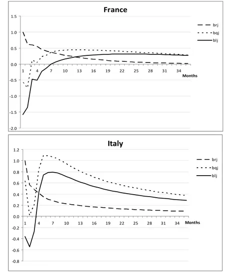
Figure 1, which will be explained in detail later, illustrates the point dramatically. The chart plots estimates based on a vector autoregression for the U.S. relative to data constructed as a weighted average of the other G7 countries. The line labeled bQj shows the estimates of the slope coefficient of a regression of the real exchange rate in period t+j on the U.S.-Foreign real interest differential in period t. When the U.S. real interest rate is relatively high, the dollar tends to be strong in real terms (the real exchange rate is below its long run mean.) Over the ensuing months, in the short run, the dollar on average appreciates even more when the U.S. real interest rate is high, before depreciating back toward its long-run mean. The other two lines in the chart represent hypothetical behavior of the real exchange rate implied under two different models.

The line labeled bRj shows how the real exchange rate would behave if uncovered interest parity held (based on the VAR forecasts of future real interest differentials.) Relative to the interest parity norm, the actual real exchange rate behavior is notably different: when the U.S. real interest rate is high, (1) the real value of the dollar is stronger than implied by interest parity (the real exchange rate is lower); (2) the dollar continues to appreciate in the short run (while interest parity implies a depreciation.) The line labeled Model illustrates the implied behavior of the real exchange rate in a class of models based on risk averse behavior of single agents in each

economy. The models have been developed to account for the uncovered interest parity puzzle – the depreciation of the currency that tends to accompany a relatively high Home interest rate.

Referring to the line labeled bQj, the models are built to explain the initial negative slope of the line. However, the models miss the overall picture badly, because they predict the effect of

interest rates on the level of real exchange rates with the wrong sign and therefore get the subsequent dynamics wrong as well.¹

The literature on the forward premium anomaly is vast. Classic early references include Bilson (1981) and Fama (1984). Engel (1996) surveys the early work that establishes this puzzle, and discusses the problems faced by the literature that tries to account for the regularity.

There have been many recent important contributions, including prominent papers by Backus, Foresi, and Telmer (2002), Lustig and Verdelhan (2007), Burnside et al. (2010a, 2010b),

Verdelhan (2010), Bansal and Shaliastovich (2010), Backus et al. (2010). Below, we survey the implications of the recent theoretical work for real exchange rate behavior.

Dornbusch (1976) and Frankel (1979) are the original papers to draw the link between real interest rates and real exchange rates in the modern, asset-market approach to exchange rates. The connection has not gone unchallenged, principally because the persistence of real exchange rates and real interest differentials makes it difficult to establish their comovement with a high degree of uncertainty. For example, Meese and Rogoff (1988) and Edison and Pauls (1993) treat both series as non-stationary and conclude that evidence in favor of cointegration is weak. However, more recent work that examines the link between real interest rates and the real exchange rate, such as Engel and West (2006), Alquist and Chinn (2008), and Mark (2009), has tended to reestablish evidence of the empirical link. Another approach connects surprise changes in real interest rates to unexpected changes in the real exchange rate. There appears to be a strong link of the real exchange rate to news that alters the expected real interest differential – see, for example, Faust et al. (2007), Andersen et al. (2007) and Clarida and Waldman (2008).

The behavior of exchange rates and interest rates described here is closely associated with the notion of “delayed overshooting”. The term was coined by Eichenbaum and Evans (1995), but is used to describe a hypothesis first put forward by Froot and Thaler (1990). Froot and Thaler’s explanation of the forward premium anomaly was that when, for example, the Home interest rate rises, the currency appreciates as it would in a model of interest parity such as Dornbusch’s (1976) classic paper. But they hypothesize that the full reaction of the market is delayed, perhaps because some investors are slow to react to changes in interest rates, so that the currency keeps on appreciating in the months immediately following the interest rate increase.

1 The models referred to here tend to treat the real exchange rate as nonstationary, in contrast to the evidence we present in section 2. As explained below, the line in Figure 2 refers to the model’s prediction for the stationary component of the real exchange rate.

Bacchetta and van Wincoop (2010) build a model based on this intuition. Much of the empirical literature that has documented the phenomenon of delayed overshooting has focused on the response of exchange rates to identified monetary policy shocks.² But in the original context, the story was meant to apply to any shock that leads to an increase in relative interest rates. Risk- based explanations of the interest parity puzzle have not confronted this literature’s finding that high interest rate currencies are strong currencies. Our empirical findings are consistent with Froot and Thaler’s hypothesis of delayed overshooting, but with one important modification.

The empirical methods here allow us to uncover what the level of the real exchange rate would be if uncovered interest parity held, and to compare the actual real exchange rate with this notional level. We find the level of the real exchange rate is excessively sensitive to real interest differentials. That is, when a country’s real interest rate increases, its currency appreciates more than it would under uncovered interest parity. Then it continues to appreciate for a number of months, before slowly depreciating back to its long run level.

Section 1 develops the approach of this paper. Section 2 presents empirical results.

Section 3 develops some general conditions that have to be satisfied in order to account for our empirical findings. We discuss the difficulties that “representative agent” models face, and illustrate the problem by showing that some recent models based on non-standard preferences are unable to match the key facts we develop.³ In section 4, we consider various caveats to our findings. Finally, in the concluding section, we discuss features of models that may be able to account for these empirical regularities.

1. Excess Returns and Real Exchange Rates

We develop here a framework for examining behavior of excess returns and the level of the real exchange rate. The approach developed here is essentially mechanical. We relate the concepts here to economic theories of risk and return in section 3.

Our set-up will consider a Home and Foreign country. In the empirical work of section 2, we always take the US as the Home country (as does the vast majority of the literature), and

2 See, for example, Eichenbaum and Evans (1995), Kim and Roubini (2000), Faust and Rogers (2003), Scholl and Uhlig (2008), and Bjornland (2009).

3 “Representative agent models” may be an inadequate label for models of the risk premium that are developed off of the Euler equation of agents with the minimum variance stochastic discount factor, generally taking the

consider other major economies as the Foreign country. Let i_t be the one period nominal interest in Home. We denote Foreign variables throughout with a superscript *, so i_t^* is the Foreign interest rate. s_t denotes the log of the foreign exchange rate, expressed as the Home currency price of Foreign currency. E s_{t t1} refers to the expectation, conditional on time t

information, of the log of the spot exchange rate at time t1. We define the “excess return”, _t, as:

(1) _t  i_t^* E s_{t t1} s i_{t t}.

This definition of excess returns corresponds with the definition in the literature. We can interpret i_t^*E s_{t t1}s_t as a first-order log approximation of the expected return in Home

currency terms for a Foreign security. As Engel (1996) notes, the first-order log approximation may not really be adequate for appreciating the implications of economic theories of the excess return. For example, if the exchange rate is conditionally log normally distributed, then



1



1 ¹2 1

ln E S_t( _t / )S_t E s_{t t}  s_t var (_t s_t ), where var (_t s_t1) refers to the conditional variance of the log of the exchange rate. Engel (1996) points out that this second-order term is approximately the same order of magnitude as the risk premiums implied by some economic models. However, we proceed with analysis of _t defined according to equation (1) both because it is the object of almost all of the empirical analysis of excess returns in foreign exchange markets, and because the theoretical literature that we consider in section 3 seeks to explain _t as defined above including possible movements in var (_t s_t1).

The well-known uncovered interest parity puzzle comes from the empirical finding that the change in the log of the exchange rate is negatively correlated with the Home less Foreign interest differential, i i_t _t^*. That is, estimates of cov(s_t1s i i_t, _t _t^*) cov( E s_{t t1}s i i_t, _t  _t^*) tend to be negative. As Engel (1996) surveys, and subsequent empirical work confirms, this finding is consistent over time among pairs of high-income, low-inflation countries.⁴ From equation (1), we note that the relationship cov(E s_{t t1}s i i_t, _t _t^*) 0 is equivalent to

* *

cov( ,_t i i_t _t) var(i i_t _t) 0 . That is, when the Home interest rate is relatively high, so i i_t _t^*

4 Bansal and Dahlquist (2000) find that the relationship is not as consistent among emerging market countries, especially those with high inflation.

is above average, the excess return on Home assets also tends to be above average: _t is below average. This is considered a puzzle because it has been very difficult to find plausible

economic models that can account for this relationship.

Let p_t denote the log of the consumer price index at Home, and _t1 p_t1p_t is the inflation rate. The log of the real exchange rate is defined as q_t  s_t p_t^*p_t. The ex ante real one-period interest rates, Home and Foreign, are given by r_t  i_t E_t_t1 and r_t^* i_t^* E_{t t}^*_1. Note also E q_{t t1} q_t E s_{t t1} s_t E_t_t^*_1E_t_t1. We can rewrite (1) as:

(2) _t   r_t^* r E q_{t t t1}q_t.

We take as uncontroversial the proposition that the real interest differential, r r_t _t^*, and excess returns, _t, are stationary random variables without time trends, and denote their means as r and  , respectively. We will also stipulate that there is no deterministic time trend or drift in the log of real exchange rates, so that the unconditional mean of E q_{t t1}q_t is zero. Rewriting (2):

(3) q_tE q_{t t1}    (r r_{t t}^* r) ( _t ).

Iterate equation (3) forward, applying the law of iterated expectations, to get:

(4) ^qt^lim_j



^{E qt t j}



   ^{Rt t}, where

(5) ^*

0

( )

t t t j t j

j

R ^ E r_ r_ r







  ^{, and}

(6)

0

( )

t t t j

j

E  







 



 ^.

We label R_t as the “prospective real interest differential”. It is the expected sum of the current and all future values of the Home less Foreign real interest differential (relative to its unconditional mean). It is important to note that R_t is not the real interest differential on long- term bonds, even hypothetical infinite-horizon bonds. R_t is the difference between the real return from holding an infinite sequence of short-term Home bonds and the real return from the infinite sequence of short-term Foreign bonds. An investment that involves rolling over short term assets has different risk characteristics than holding a long-term asset. Hence we coin the

phrase “prospective” real interest differential to avoid the trap of calling R_t the long-term real interest differential.

Similarly, _t is the expected infinite sum of excess returns on the Foreign security. We label this the “prospective excess return”.

The left-hand side of (4), ^qt^lim_j



^{E qt t j}



, can be interpreted as the transitory component of the real exchange rate. In fact, according to our empirical findings reported in section 2, we can treat the real exchange rate as a stationary variable, so ^lim_j



^{E qt t j}



^q. As is well known, even if the real exchange rate is stationary, it is very persistent. Engel (2000), in fact, argues that it may be practically impossible to distinguish between the stationary case and the unit root case under plausible economic conditions. We proceed in examining q_tq, assuming stationarity, but note that our methods could be applied to the transitory component of the real exchange rate, taken as the difference between q_t and a measure of the permanent component, ^lim_j



^{E qt t j}



. In section 4, we note how Engel’s (2000) interpretation implies that in practice it may not be possible to distinguish a permanent and transitory component, but make the case that the economic analysis of that paper argues for treating the real exchange rate as stationary.

In section 3, we discuss the common assumption in theoretical models of excess returns that the real exchange rate is equal to the difference between the marginal utility of a (particular) Home consumer and (particular) Foreign consumer. We note here that stationarity of the real exchange rate is completely compatible with a unit root in the log of consumption, or in the marginal utility of consumption. It requires simply that Home and Foreign marginal utilities of consumption be cointegrated, which is a natural condition among well-integrated economies such as the highly developed countries used in this study. It is analogous to the assumption made in almost all closed-economy models that we can treat the marginal utilities of different

consumers within a country as cointegrated.

Under the stationarity assumption, we can write (4) as:

(7) q q_t    R_{t t}.

From this formulation, we see that the prospective excess return, _t, captures the potential effect of risk premiums on the level of the real exchange rate, holding the prospective real interest differential constant.

In the next section, we present evidence that cov( ,R r r_{t t} _t^*) 0 and cov( ,_t r r_t _t^*) 0 . Taken together, these two findings imply from (7) that cov( ,q r r_{t t} _t^*) 0 , which jibes with the concept familiar from Dornbusch (1976) and Frankel (1979) that when a country’s real interest rate is high (relative to the foreign real interest rate, relative to average), its currency tends to be strong in real terms (relative to average.) But if cov( ,_t r r_t _t^*) 0 , the strength of the currency cannot be attributed entirely to the prospective real interest differential, as it would be in

Dornbusch and Frankel (who both assume uncovered interest parity, or that _t 0.) The relationship between excess returns and real interest differential plays a role in determining the relation between the real exchange rate and real interest rates.

It is entirely unsurprising that we find cov( ,R r r_{t t} _t^*) 0 . This simply implies that there is not a great deal of non-monotonicity in the adjustment of real interest rates toward the long run mean.

The central puzzle raised by this paper concerns the two findings, cov( ,_t r r_t _t^*) 0 and cov( ,_t r r_t _t*) 0 . The short-run excess return on the Foreign security, _t, is negatively correlated with the real interest differential, consistent with the many empirical papers on the uncovered interest parity puzzle. But the prospective excess return, _t, is positively correlated.

Given the definition of _t in equation (6), we must have that for at least j0 and possibly for some j0, cov(E_{t t j}_ ,r r_t _t^*) 0 , but for other j0, cov(E_{t t j}_ ,r r_t _t^*) 0 . The sum of the latter covariances must exceed the sum of the former to generate cov( ,_t r r_t _t^*) 0 . As we discuss in section 3, our risk premium models of excess return are not up to the task of

explaining this finding. In fact, while they are constructed to account for cov( ,_t r r_t _t^*) 0 , they have the counterfactual implication that cov( ,_t r r_t _t^*) 0 .

The empirical approach of this paper can be described simply. We estimate VARs in the variables q_t, i i_t _t^*, and i_t1i_t^*_1( _t _t^*). From the VAR estimates, we construct measures of



^{* ( 1 *1)}



^*

t t t t t t t

E i  i _ _  r r . Using standard projection formulas, we can also construct estimates of R_t. To measure _t, we take the difference of q_tq and R_t. From these VAR estimates, we calculate our estimates of the covariances just discussed. As an alternative approach, we estimate VARs in q_t, i i_t _t^*, and  _t  _t^*, and then construct the needed estimates of r r_t _t^*, R_t, and _t. The estimated covariances under this alternative approach are very similar to those from the original VAR. Our approach of estimating undiscounted expected present values of interest rates from VARs is presaged in Mark (2009) and Brunnermeier et al.

(2009).

2. Empirical Results

We investigate the behavior of real exchange rates and interest rates for the U.S. relative to the other six countries of the G7: Canada, France, Germany, Italy, Japan, and the U.K. We also consider the behavior of U.S. variables relative to an aggregate weighted average of the variables from these six countries.⁵ Our study uses monthly data. Foreign exchange rates are noon buying rates in New York, on the last trading day of each month, culled from the daily data reported in the Federal Reserve historical database. The price levels are consumer price indexes from the Main Economic Indicators on the OECD database. Nominal interest rates are taken from the last trading day of the month, and are the midpoint of bid and offer rates for one-month Eurorates, as reported on Intercapital from Datastream. The interest rate data begin in June 1979. Most of our empirical work uses the time period June 1979 to October 2009. In some of the tests for a unit root in real exchange rates, reported below, we use a longer time span from June 1973 to October 2009. It is important for our purposes to include these data well into 2009 because it has been noted in some recent papers that there was a crash in the “carry trade” in 2008, so it would perhaps bias our findings if our sample ended prior to this crash.⁶

5 The weights are determined by the value of each country’s exports and imports as a fraction of the average value of trade over the six countries.

6 See, for example, Brunnermeier, et al. (2009) and Jordà and Taylor (2009).

2.1 Tests for unit root in real exchange rates

It is well known that real exchange rates among advanced countries are very persistent.⁷ There is no consensus on whether these real exchange rates are stationary or have a unit root. Two recent studies of uncovered interest parity, Mark (2010) and Brunnermeier, et al. (2009) estimate statistical models that assume the real exchange rate is stationary, but do not test for stationarity.

Jordà and Taylor (2010) demonstrate that there is a profitable carry-trade strategy that exploits the uncovered interest parity puzzle when the trading rule is enhanced by including a forecast that the real exchange rate will return to its long-run level when its deviations from the mean are large. That paper assumes a stationary real exchange rate and includes statistical tests that cannot reject cointegration of s_t with p_tp_t^*. However, that study does not indicate whether the cointegrating vector is insignificantly different than [1,-1], so the tests are not equivalent to a test for a unit root in q_t.

We present evidence here that favors the hypothesis of no unit root in the real exchange rate. Clearly the real exchange rate is very persistent, and the evidence in favor of stationarity is not incontrovertible.

Table 1 presents standard ADF tests for a unit root. The null is not rejected for any currency except the U.K. pound at the 10 percent level. The table also includes tests for a unit root based on the GLS test proposed by Elliott et al. (1996). These tests show stronger evidence against a unit root – the null is rejected at the 5% level for three currencies, at the 10% level for two others, and not rejected for the Canadian dollar or Japanese yen. However, the test statistic is based on the assumption that there may be a trend in the real exchange rate under the

alternative, which is not a realistic assumption for these real exchange rates.

We next follow much of the recent literature on testing for a unit root in real exchange rates by exploiting the power from panel estimation. The lower panel of Table 1 reports estimates from a panel model. The null model in this test is:

(8) _{1 1}

1

( )

ki

it it i i it j it j it

j

q q_  c q _ q_{ } 



  



  ^.

Under the null, the change in the real exchange rate for country i follows an autoregressive process of order k_i. Note that the parameters and the lag lengths can be different across the currencies. Under the alternative:

(9) _{1 1 1}

1

( )

ki

it it i it i it j it j it

j

q q _  q _ c q _ q _{ } 



   



  ^,

with a common  for the currencies.

We estimate  for the six currencies from (9).⁸ We find the lag length for each currency by first estimating a univariate version of (9), and using the BIC criterion. The estimated value of  is reported in the lower panel of Table 1, in the row labeled “no covariates”.

This table also reports the bootstrapped distribution of . The bootstrap is constructed by estimating (8), then saving the residuals for the six real exchange rates for each time period.

We then construct 5000 artificial time series (each of length 440, corresponding to our sample of 440 months) for the real exchange rate by resampling the residuals and using the estimates from (8) to parameterize the model.

The lower panel of Table 1, in the row labeled “no covariates” reports certain points of the distribution of  from the bootstrap. We see that we can reject the null of a unit root at the 5 percent level.

We also consider a version of the panel test in which we include covariates. Specifically, we investigate the possibility that the inflation differential (with the U.S.) helps account for the dynamics of the real exchange rate. We follow the same procedure as above, but add lagged own relative inflation terms to equation (9). To generate the distribution of the estimate of , we estimate a VAR in the change in the real exchange rate (as in (8)) and the inflation rate. For each country, the real exchange rate and inflation rates depend only on own-country lags under the null. The bootstrap proceeds as in the model with no covariates.

The bottom panel of Table 1 reports the estimated  and its distribution for the model with covariates in the row labeled “with covariates”. Adding covariates does not alter the conclusion that we can reject a unit root at the 5 percent level.

Based on these tests, we will proceed to treat the real exchange rate as stationary, though we note that the evidence favoring stationarity is thin for the Canadian dollar and Japanese yen real exchange rates.

8 We do not include the average G6 real exchange rate as a separate real exchange rate in this test.

2.2 Fama regressions

Table 2 reports results from the standard “Fama regression” that is the basis for the forward premium puzzle. The change in the log of the exchange rate between time t+1 and t is regressed on the time t interest differential:

(10) s_t1 s_t _s_s(i i_t _t^*)u_{s t, 1} .

Under uncovered interest parity, _s 0 and _s 1. We can rewrite this regression as:

* *

1 , 1

( _ )  (1  )( ) _

        

t t t t s s t t s t

i i s s i i u .

The left-hand side of the regression is the ex post excess return on the home security. If _s 0 but _s 1, then the high-interest rate currency tends to have a higher excess return. There is a positive correlation between the excess return on the Home currency and the Home-Foreign interest differential.

The Table reports the 90% confidence interval for the regression coefficients, based on Newey-West standard errors. For five of the six currencies, the point estimate of _s is negative (Italy being the exception). Of those five, the 90% confidence interval for _s lies below one for four (France being the exception, where the confidence interval barely includes one.) For four of the six, zero is inside the 90% confidence interval for _s. (In the case of the U.K., the

confidence interval barely excludes zero, while for Japan we find strong evidence that _s is greater than zero.)

The G6 exchange rate (the weighted average exchange rate, defined in the data section) appears to be less noisy than the individual exchange rates. In all of our tests, the standard errors of the coefficient estimates are smaller for the G6 exchange rate than for the individual country exchange rates, suggesting that some idiosyncratic movements in country exchange rates gets smoothed out when we look at averages. Table 2 reports that the 90% confidence interval for this exchange rate lies well below one, with a point estimate of -1.467.⁹

2.3 Fama regressions in real terms

The Fama regression in real terms can be written as:

(11) q_t1 q_t _q_q(r rˆ ˆ_t _t^*)u_{q t, 1} .

In this regression, r rˆ ˆ_t _t^* refers to estimates of the ex ante real interest rate differential,

* * *

1 ( 1)

t t t t t t t t

r r  i E_  i E_ and. We estimate the real interest rate from VARs. As noted above, we consider two different VAR models. Model 1 is a VAR with 3 lags in the variables q_t , i i_t _t^*, and i_t1i_t^*_1( _t _t^*). From the VAR estimates, we construct measures of



^{* ( 1 *1)}



^*

t t t t t t t

E i  i _ _  r r . Model 2 is a 3-lag VAR in q_t, i i_t _t^*, and  _t _t^*.

There are two senses in which our measures of r rˆ ˆ_t _t^* are estimates. The first is that the parameters of the VAR are estimated. But even if the parameters were known with certainty, we would still only have estimates of r r_t _t^* because we are basing our measures of r r_t _t^* on linear projections. Agents certainly have more sophisticated methods of calculating expectations, and use more information than is contained in our VAR.

The findings for the Fama regression in real terms are similar to those when the

regression is estimated on nominal variables. For four of the six currencies, the estimates of _q, reported in Table 3A, are negative, and all are less than one. In addition, the estimated

coefficient for the G6 aggregate is close to -1. This summary is true for both VAR models.

Table 3A reports three sets of confidence intervals. All of the subsequent tables also report three sets of confidence intervals for each parameter estimate. The first is based on Newey-West standard errors, ignoring the fact that r rˆ ˆ_t _t^* is a generated regressor. The second two are based on bootstraps. The first bootstrap uses percentile intervals and the second percentile-t intervals.¹⁰

From Table 3A, all three sets of confidence intervals are similar. For the individual currencies, for both Model 1 and Model 2, the confidence interval for _q lies below one for Germany, Japan, and the U.K. It contains one for Canada and Italy, and contains one for France except using the second confidence interval.

10 See Hansen (2010). The Appendix describes the bootstraps in more detail.

The findings are clear using the G6 average exchange rate: the coefficient estimate is

0.93 when the real interest estimate comes from Model 1, and 0.91. All of the confidence intervals lie below one, though they all contain zero. For both models, the estimate of _q ^{is very} close to zero, and all confidence intervals contain zero.

In summary, the evidence on the interest parity puzzle is similar in real terms as in nominal terms. The estimate of the coefficient _q, tends to be negative and there is strong evidence that it is less than one. Even in real terms, the country with the higher interest rate tends to have short-run excess returns (i.e., excess returns and the interest rate differential are positively correlated.)

The Fama regression finds a strong negative correlation between s_t1s_t and i i_t _t^*. It is well known that for the currencies of low-inflation, high-income countries, s_t1s_t is highly correlated with q_t1q_t, which suggests q_t1q_t is negatively correlated with i i_t  _t^*. Since

* * *

1 1

( )

t t t t t t

i i   r r E _ _ , for exploratory reasons we consider a regression of q_t1q_t on ˆ ˆ_{t t}*

r r and Eˆ (_t _t1_t^*_1), where the latter is our measure of the expected inflation differential generated from the VARs. These regressions are reported in Table 3B. Specifically, Table 3B reports the estimation of:

(12) q_t1q_t _q _q1(rˆ_trˆ_t^*)_q2E^ˆ_t(_t1_t^*_1)u_{q t, 1} .

The estimates of _q1 tend to be negative, and generally more negative than those reported in Table 3A for equation (11). The real surprise from Table 3b is that the estimates of

_q2 are negative for all currencies in both models. Though they are not always significantly negative individually, and we do not calculate a test of their joint significance, it is nonetheless telling that all of the coefficient estimates are negative. This implies that the currency of the country that is expected to have relatively high inflation is expected to appreciate in real terms.

We return to this finding in section 5.

2.4 The real exchange rate, real interest rates, and the level risk premium Table 4 reports estimates from

(13) q_t _q_q(r rˆ ˆ_t _t^*)u_{q t,} .

In all cases (all currencies, for both Model 1 and Model 2), the coefficient estimate is negative.

In virtually all cases, although the confidence intervals are wide, the coefficient is significantly negative.¹¹

Recall from equation (7) that q q_t    R_{t t}, where ^*

0

( )

t t t j t j

j

R E r r r



 







  ^and

0

( )

t t t j

j

E  







 



 . If there were no excess returns, so that q_t  q R_t, and r rˆ ˆ_t _t^* were positively correlated with R_t, then there is a negative correlation between q_t and r rˆ ˆ_t  _t^*. That is, under uncovered interest parity, the high real interest rate currency tends to be stronger. For example, this is the implication of the Dornbusch-Frankel theory in which real interest differentials are determined in a sticky-price monetary model.

But we can make a stronger statement – there is a relationship between the real interest differential, r rˆ ˆ_t _t^*, and our measure of the level risk premium, ^ˆ_t (where ^ˆ_t is our estimate of

t based on the VAR models.) Our central empirical finding is reported in Table 5. This table reports the regression:

(14)  ^ˆ_t __(rˆ_trˆ_t^*)u_t.¹²

In all cases, the estimated slope coefficient is positive. The 90 percent confidence intervals are wide, but with a few exceptions, lie above zero. The confidence for the G6 average strongly excludes zero. To get an idea of magnitudes, a one percentage point difference in annual rates between the home and foreign real interest rates equals a 1/12^th percentage point difference in monthly rates. The coefficient of around 32 reported for the regression when we take the U.S.

relative to the average of the other G7 countries translates into around a 2.7% effect on the level risk premium. That is, if the U.S. real rate increases one annualized percentage point above the

11 The exceptions are that the third confidence interval contains zero for Model 1 for France, and Models 1 and 2 for the U.K.

12 To be precise, ˆ_t is calculated as the difference between q_t and our VAR estimate of R_t. To calculate our estimate of R_t, given by the infinite sum of equation (5), we demean r_{t j} r_{t j}^*_ by its sample mean. We use the sample mean rather than maximum likelihood estimate of the mean because it tends to be a more robust estimate.

real rate in the other countries, the dollar is predicted to be 2.7% stronger in real terms from the level risk premium effect.

This finding is surprising in light of the well-known uncovered interest parity puzzle. In the previous two subsections, we have documented that when r r_t _t^* is above average, the Home currency tends to have excess returns. That seems to imply that the high interest rate currency is the riskier currency. But the estimates from equation (14) deliver the opposite message – the high interest rate currency has the lower level risk premium. _t is the level risk premium for the Foreign currency – it is positively correlated with r r_t _t^*, so it tends to be high when r_t^*r_t is low.

Recall that the level risk premium is defined in equation (6) as

0

( )

t t t j

j

E  







 



 ^{. We}

have then that

(15) ^{* *}

0

cov( ,_{t t t} ) cov[ (_{t t j}), _{t t} ]

j

r r ^ E _ r r



  



 ^.

The short-run interest parity puzzle establishes that cov( ,_t r r_t _t^*) 0 . Clearly if

cov( ,_t r r_t _t*) 0 , then we must have cov[ (E_t _{t j} ),r_tr_t^*] 0 for at least some j0. That is, in order for cov( ,_t r r_t _t^*) 0 , we must have a reversal in the correlation of the short-run risk premiums with r r_t _t^* as the horizon extends.

This is illustrated in Figure 2, which plots estimates of the slope coefficient in a regression of Eˆ (_t _{t j 1}) on r rˆ ˆ_t _t^* for j1, ,100K :

* ,

1 ( )

ˆ (_t _{t j} )_j_j r r_t _t  _^j_t

E u

For the first few j, this coefficient is negative, but it eventually turns positive at longer horizons.

The Figure also plots the slope of regressions of E rˆ (_{t t j 1}r_{t j}^*_{ 1}) on r rˆ ˆ_t _t^* for 1, ,100

j K :

* *

1 1 ,

ˆ (_{t t j }  _{t j } )_rj_rj(_t _t ) _{r t}^j

E r r r r u

These tend to be positive at all horizons.

The Figure also includes a plot of the slope coefficients from regressing E qˆ (_{t t j} q_{t j 1}) for 1, ,100

j K :

*

1 ,

ˆ (_{t t j}  _{t j } )_qj_qj(_t _t ) _{q t}^j

E q q r r u

Since E qˆ_t( _{t j} q_{t j 1})E rˆ_t(_{t j 1}r_t^*_{ j 1})Eˆ_t(_{t j 1}), these regression coefficients are simply the sum of the other two regression coefficients that are plotted. In this case, the regression

coefficients start out negative for the first few months, but then turn positive for longer horizons.

To summarize, when the Home real interest rate relative to the Foreign real interest rate is higher than average, the Home currency is stronger in real terms than average. Crucially, it is even stronger than would be predicted by a model of uncovered interest parity. Excess returns or the foreign exchange risk premium contribute to this strength. If Home’s real interest rate is high – in the sense that the Home relative to Foreign real interest rate is higher than average – the level risk premium on the Foreign security is higher than average.

We can project the future path of the real exchange rate when Home real interest rates are high using the facts that the currency tends to be stronger than average (the finding of regression (14)), that it continues to appreciate in the short run (the famous puzzle, confirmed in the

findings from regression (11)), and that the real exchange rate is stationary so it is expected to return to its unconditional mean (established in Table 1.) When the Home real interest rate is high, the Home currency is strong in real terms, and expected to get stronger in the short run.

However, eventually it must be expected to depreciate back to its long run level.

One implication of these dynamics is similar to Jorda and Taylor’s (2009) findings about forecasting nominal exchange rate changes. They find that the nominal interest differential can help to predict exchange rate changes in the short run: the high interest rate currency is expected to appreciate (contrary to the predictions of uncovered interest parity.) But the forecasts of the exchange rate can be enhanced by taking into account purchasing power parity considerations.

The deviation from PPP helps predict movements of the nominal exchange rate as the real exchange rate adjusts toward its long-run level.