CEEC Growth Projections: Certainly Necessary and Necessarily Uncertain Martin Wagner Jaroslava Hlouskova 04-03 February 2004

(1)

Diskussionsschriften

CEEC Growth Projections: Certainly Necessary and Necessarily Uncertain

Martin Wagner Jaroslava Hlouskova

04-03 February 2004

Universität Bern

Volkswirtschaftliches Institut Gesellschaftstrasse 49 3012 Bern, Switzerland

(2)

CEEC Growth Projections: Certainly Necessary and Necessarily Uncertain

^∗

Martin Wagner^†

Department of Economics University of Bern Gesellschaftsstrasse 49

CH-3012 Bern

Jaroslava Hlouskova

Department of Economics and Finance Institute for Advanced Studies

Stumpergasse 56 A-1060 Vienna

February 17, 2004

Abstract

In this paper we discuss the necessity for an indirectapproach to assess the growth and

convergence prospects of ten Central and Eastern European countries (CEEC10). The necessity for an indirect approach arises for two reasons. First, the ongoing structural changes in the transition economies imply that their growth process is not yet adequately described by the long-run growth forces as identified by (neoclassical) growth theory.

Second, their upcoming European Union membership has to be taken into account in growth projections.

The indirect approach proposed in this paper is to base the growth projections for the CEEC10 on growth equations estimated for the incumbent EU member states. Thus, in effect we propose a calibration approach. Our study differs from previous studies that employ an indirect approach in two ways. First, we estimate growth equations for the EU and not for a large world-wide country data set that contains many heterogeneous countries that are essentially unrelated to the CEECs. Second, we assess the uncertainty inherent in growth projections by estimating a variety of economically meaningful equations and by specifying a variety of plausible scenarios for the explanatory variables. This results in distributions of projected growth rates, which allow for an uncertainty analysis.

Besides growth rate distributions also convergence times distributions are computed.

JEL Classification: F02, O40, O57, P21, P27

Keywords: Real convergence, transition economies, growth projections, uncertainty analysis

∗Financial support from the Austrian Ministry of Economic Affairs is gratefully acknowledged. The authors would like to thank H. Hutter, M. Kotov and B. Meininger for their help with TEX and data issues and C. Osbat, T. Owen and A. W¨org¨otter for valuable discussions. We would also like to thank seminar participants at the Institute for Advanced Studies, the Vienna Institute for Comparative Economic Studies (WIIW), the Osterreichische Nationalbank, the CEPR Transition Workshop in Portoroz, especially Laszlo Halpern, Miklos¨ Koren and Mark Schaffer, and at the University of Ljubljana. This paper is a substantially revised, completely re-estimated and shortened version of our CEPR Discussion Paper No. 3318 entitled ‘The CEEC10’s Real Convergence Prospects’.

†Correspondence: Tel.: ++41-31 6314778, Fax: ++41-31 6313992, Email: martin.wagner@vwi.unibe.ch.

Part of this work has been carried out whilst visiting the Economics Department of Princeton University, whose hospitality is gratefully acknowledged.

(3)

1 Introduction

Numerous studies have offered assessments of the growth perspectives of various groups of transition economies.¹ All these studies suffer from the fact that the transition process these countries are undergoing renders growth projections difficult. This stems from the obvious fact that in all transition economies huge structural changes occur on their way from cen- trally planned to market economies. For instance in all countries, initially atransformational recessionoccurred with drastic falls in output, high unemployment and often hyper inflation, see Campos and Coricelli (2002) or Kornai (1994). As Fischer and Sahay (2000) point out, the growth process in transition economies depends upon two sets of factors. The first is in relation to transition, and the second are the long-run growth forces as laid out by neoclassical growth theory. The further along a country is on its transition process, the more important the latter set of factors will be. Thus, an assessment of the growth perspectives of transition economies has to start out by displaying the importance of the two sets of factors.

For the Central and Eastern European countries (CEECs), which are the focus in this paper, the growth perspectives are also shaped by the upcoming European Union (EU) accession. Eight of the countries in our sample will join the EU in 2004, namely the Czech Republic (CZE), Estonia (EST), Hungary (HUN), Latvia (LVA), Lithuania (LTU), Poland (POL), the Slovak Republic (SVK) and Slovenia (SVN), while two, Bulgaria (BGR) and Ro- mania (ROM),²are candidates for memberships in a few years time. Thus, for these countries, long-run growth projections have to take into account the likely effects of EU membership on the new entrants’ growth process. EU membership leads toinstitutional or systemic convergence of the new entrants to the system prevalent in the incumbent EU member states.

The new entrants have to adopt theacquis communautaireand there will also be convergence in the way economic policy is conducted in the incumbent EU member states and the new entrants. Eventual entry to the European Monetary Union is mandatory for the CEECs joining the EU. In meeting the mandatory requirement to join the European Monetary Union, the CEECs must meet clear quantitative bounds on fiscal and monetary policy and will have to obey the regulations laid out in the Treaty of Maastricht. Furthermore, the already substantial degree of economic interaction between the current EU member states and the new

1Examples are Berg et al. (1999), Campos (2000), Campos and Coricelli (2002), DeMelo et al. (1997), Estrin and Urga (1997), Fischer and Sahay (2000), Fischer et al. (1998a), Fischer et al. (1998b) and Havrylyshyn et al. (1998).

2This group of countries is referred to as CEEC10 throughout the paper.

(4)

entrants is likely to increase further. Already now the EU is by far the largest trading partner and the main source of foreign direct investment in the CEECs. As a condition for joining the EU, the CEECs have to (eventually) open their goods and service markets consistent with the principles and practices of the so-calledcommon market. All these effects can be expected to lead to substantial convergence between the incumbent and the new EU member states.

Ben-David (1993, 1996) shows that previous EU enlargements induced significant subsequent convergence. Thus, also for the CEEC10, the future growth process will be substantially shaped by the effects of EU accession. This implies that assessments of the growth perspectives for these countries have to take into account that theendpointof the transition process is known.

An indirect approach is often used in the literature for long-run growth projections, since, as discussed, up to now neoclassical growth theory does not adequately describe the growth process of transition economies like the CEEC10. This implies that growth scenarios based on equations estimated for transition countries over the last decade or so, lead to a projection of the turbulent behavior observed up to now. To address this problem, growth assessments are often based on equations estimated for large samples of countries and the resultant coefficients are combined with the values of the independent variables from the countries being studied to obtain growth rate projections. Such anindirect approach induces, by construc- tion, convergence of the sample of countries studied to the sample of countries for which the equations have been specified. E.g. Fischer et al. (1998b) use specifications of Barro (1991) and Levine and Renelt (1992) to obtain their growth rate projections for a set of thirteen transition economies.

This approach does not come without problems: First, it is based on the underlying assumption that convergence to a reference group of countries is a more likely scenario than a continuation of the observed patterns. Second, the relevance of thecalibration procedure has to be addressed. Third, the specification uncertainty inherent in the growth and convergence literature (see e.g. Sala-i-Martin, 1997) has to be taken into account. This paper addresses these three main problems as follows: First, due to the upcoming EU accession, convergence of the new entrants towards the incumbent member states is more likely to be a determinant of the future growth process than a continuation of the trends seen thus far. Thus, some sort of indirect approach is indeed necessary. Second, we estimate growth equations only for the current EU member states and not for large samples that include many countries at

(5)

heterogeneous levels of development that are essentially unrelated economically to the CEECs.

This reflects the assumption of asystemic convergence of the CEECs towards the EU in its current boundaries as compared to convergence towards the ‘statistical mean country’ from a world-wide sample. To be precise, the estimations of the growth equations are performed for the EU14 (the current EU15 excluding Luxembourg). Luxembourg is excluded because of its small size, its dissimilarity with any of the CEECs and some problems with data availability. Third, the specification uncertainty is quantified by specifying a variety of growth equations, 18 in total.³ This is combined with aneconomic robustness analysis by specifying 7 scenarios for economically important explanatory variables: the government consumption and the investment shares. This results in a total of 126 growth rate projections for each of the CEEC10, which allows the estimation of the distributions, respectively the densities, of the growth rate projections. The distribution of growth rates forms the basis for assessing the uncertainty inherent in the projections.

Based on growth rate distributions, we also compute convergence time distributions. We discuss convergence time distributions with respect to various country groups: the EU14, the EU24 (i.e. the EU14 plus the CEEC10), and the cohesion countries Greece, Portugal and Spain (C3). In addition to convergence time distributions, two scenarios are discussed in detail: The mean scenario, based on the mean convergence times, and the optimistic scenario, based on the first deciles of the convergence time distributions. The convergence time computations are computed with the assumption that the EU14 and the C3 continue to grow at their historical averages over the period 1990–2001. A separate appendix available upon request contains similar computations with the growth rates assumed for the EU14 and the C3 given by the mean growth rates from the 18 equations.

The results are discussed in detail in Section 4. A brief overview of the results indicates that the growth rate distributions are bimodal. The mean growth rates vary from 3.05% p.a.

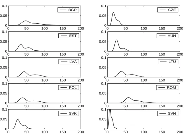
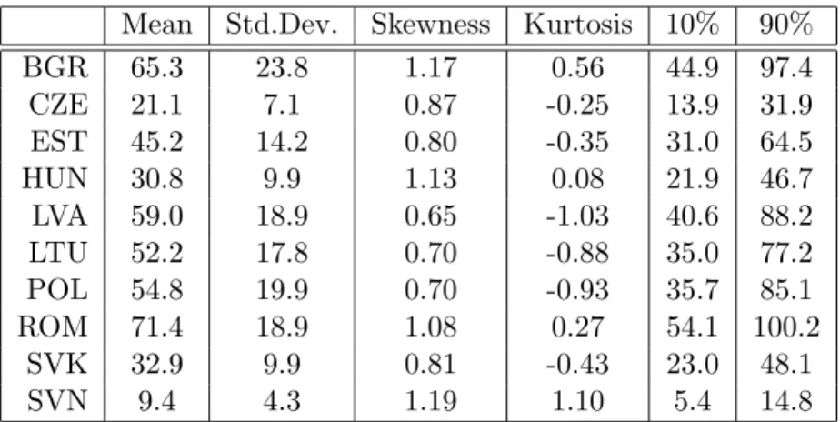
for Slovenia to 3.52% p.a. for Romania. The standard deviation of the growth rate distributions is around 0.5% annual growth for all countries. Considering for example convergence times to 80% of the income level of the EU14,⁴ the results range from a mean convergence time of 9.4 years (standard deviation 4.3 years) for Slovenia to 65.3 years (standard deviation

3The equations are estimated by panel methods, and not only cross-sectionally, as is common in the empirical growth literature.

4With the assumption that the EU14 continue to grow at the average growth rate of real per capita GDP observed over the period 1990–2001, namely 1.74%.

(6)

23.8 years) for Bulgaria. We thus find mean convergence times that are in line with some of the point estimates available in the literature. However, there is a substantial degree of uncertainty around these point estimates, which is highlighted by our analysis.

The paper is organized as follows: Section 2 discusses the growth process in the CEEC10 over the period 1991–2001. In Section 3 the growth process in the EU14 and the resulting growth or convergence equations are discussed. Section 4 contains the resulting growth and convergence scenarios for the CEEC10 and Section 5 provides a summary and conclusions.

Appendix A contains a description of the data. Some additional empirical results are reported in Appendix B.

2 The Growth Performance of the CEEC10

In this section we briefly review the growth performance of the CEEC10 over the period 1991–

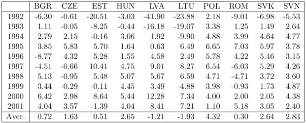
2001.⁵ Table 1 displays the growth rates of real per capita GDP. As already mentioned in the introduction, the beginning of transition has been characterized by large output losses, the most drastic example being a fall in real per capita GDP in Latvia by 41.9% from 1991 to 1992.

The Baltic countries have been more severely hit by the dissolution of the Soviet Union, which restrained accessibility of in- and output markets, than other transition economies (compare Blanchard and Kremer, 1997). The table also shows that with the exception of the two reform laggards Bulgaria and Romania, and to a certain extent the Czech Republic, the countries in our sample have achieved relatively good growth performance after the initial recession. The last row of Table 1 displays the average growth rate over the period, which is positive with the exception of Latvia and Lithuania. This is equivalent to saying that the initial output losses in these two countries were so large that, despite their sound recent growth performance, they have not yet reached their 1991 income levels. The largest average growth rate is observed for Poland, with 4.32%, see DeBroeck and Koen (2000) for a detailed account of the Polish experience.⁶

The recent sound growth performance of the CEEC10 might suggest that the mechanisms laid out by the standard neoclassical growth model, see Ramsey (1928), Solow (1956) or Cass

5More detailed data analysis and empirical investigations are available from the authors upon request or in the working paper Wagner and Hlouskova (2002). See also the detailed account of the growth performance of transition economies given in Campos and Coricelli (2002) and the references therein.

6Note also that output declined in Poland already before the start of our sample period, which biases the comparison to a certain extent.

(7)

BGR CZE EST HUN LVA LTU POL ROM SVK SVN 1992 -6.30 -0.61 -20.51 -3.03 -41.90 -23.88 2.18 -9.01 -6.98 -5.53 1993 1.11 -0.05 -8.25 -0.44 -16.18 -19.07 3.38 1.25 1.49 2.64 1994 2.79 2.15 -0.16 3.06 1.92 -9.90 4.88 3.99 4.64 4.77 1995 3.85 5.83 5.70 1.64 0.63 6.49 6.65 7.03 5.97 3.78 1996 -8.77 4.32 5.28 1.55 4.58 2.49 5.78 4.22 5.46 3.15 1997 -4.51 -0.66 10.41 4.75 9.01 8.27 6.54 -6.03 5.29 4.26 1998 5.13 -0.95 5.48 5.07 5.67 6.59 4.71 -4.71 3.72 3.60 1999 3.44 -0.29 -0.11 4.45 3.49 -4.88 3.98 -0.93 1.73 4.87 2000 6.42 2.98 8.64 5.44 12.28 7.34 4.00 2.00 2.05 4.38 2001 4.04 3.57 -1.39 4.04 8.41 7.21 1.10 5.18 3.05 2.40 Aver. 0.72 1.63 0.51 2.65 -1.21 -1.93 4.32 0.30 2.64 2.83

Table 1: Growth rates of real per capita GDP.

(1965), provides an apt description of the growth performance by now.⁷

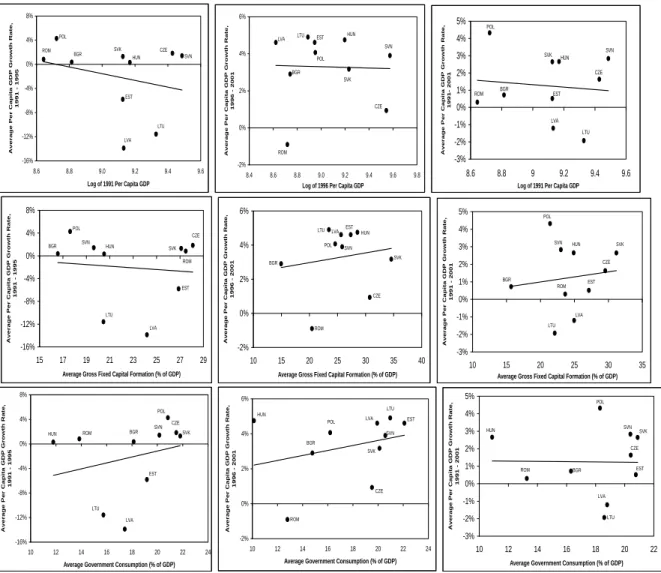
The standard neoclassical growth model, as well as a variety of extensions, have clear implications concerning the (long-run) correlations observed between key variables. To be clear, the intention is not to test or estimate a particular growth model, but merely to use growth theory as a key input that allows for a structured modelling process consistent with theory. In particular neoclassical growth theory is consistent with convergence of output across nations. This empirical fact has been observed for the EU and is likely to be extended also to the new entrants. Some key correlations derived for a set of homogenous countries include: a negative correlation between initial real per capita GDP and subsequent growth, which is usually referred to asβ-convergence; a positive correlation between the investment share and growth; and a negative correlation between the government consumption share and growth. These unconditional correlations are displayed in Figure 1. Figure 1 is structured as follows: From the top to the bottom it displaysβ-convergence or divergence, the investment share-growth correlation⁸ and the government consumption share-growth correlation. The first column corresponds to the period 1991–1995, the second to the period 1996–2001 and in

7Starting with Baumol (1986) and DeLong (1988) theconvergenceliterature has been rapidly growing, since its popularization due to Barro (1991, 1997), Barro and Sala-i-Martin (1992a, 1992b, 1995) and Sala-i-Martin (1990). For a critical assessment of the convergence literature and an apt description of its many limitations see Durlauf and Quah (1999). Bernard and Durlauf (1995, 1996) propose a time-series oriented analysis of convergence. Quah (1996a-b, 1997a-c) proposes to use Markov chain methods to study the distributional dynamics of income. Our working paper Wagner and Hlouskova (2002) contains investigations using all these methodologies. For the CEEC10, for instance, we found that over the period 1991–2001 the so-called twin- peaks property emerges. This is a reflection of the diverse income development in the CEEC10 over that period. Due to our focus in this paper, which is to assess the growth perspectives, we have excluded these further investigations.

8Investment is used as short hand for gross fixed capital formation, see Appendix A for data definitions.

(8)

SVN ROM SVK

POL

HUN CZE BGR

LVA LTU EST

-16%

-12%

-8%

-4%

0%

4%

8%

8.6 8.8 9.0 9.2 9.4 9.6

Log of 1991 Per Capita GDP

Average Per Capita GDP Growth Rate, 1991 - 1995

LTU EST LVA

BGR

CZE HUN

POL

ROM

SVK SVN

-2%

0%

2%

4%

6%

8.4 8.6 8.8 9.0 9.2 9.4 9.6 9.8

SVK SVN

ROM POL

HUN CZE

BGR

LVA LTU EST

-3%

-2%

-1%

0%

1%

2%

3%

4%

5%

8.6 8.8 9 9.2 9.4 9.6

Average Per Capita GDP Growth Rate, 1991- 2001

SVN

SVK ROM POL

HUN

CZE BGR

LVA LTU

EST

-16%

-12%

-8%

-4%

0%

4%

8%

15 17 19 21 23 25 27 29

Average Gross Fixed Capital Formation (% of GDP)

SVN SVK

ROM POL

HUN

CZE BGR

LTU LVA EST

-2%

0%

2%

4%

6%

10 15 20 25 30 35 40

EST

LTU LVA BGR

CZE HUN POL

ROM SVN SVK

-3%

-2%

-1%

0%

1%

2%

3%

4%

5%

10 15 20 25 30 35

SVN ROM SVK

POL

HUN

CZE BGR

LVA LTU

EST

-16%

-12%

-8%

-4%

0%

4%

8%

10 12 14 16 18 20 22 24

Average Government Consumption (% of GDP) Average Per Capita GDP Growth Rate, 1991 - 1995

EST LTU LVA

BGR

CZE HUN

POL

ROM

SVK SVN

-2%

0%

2%

4%

6%

10 12 14 16 18 20 22 24

SVN SVK

ROM

POL

HUN

CZE

BGR

LVA

LTU EST

-3%

-2%

-1%

0%

1%

2%

3%

4%

5%

10 12 14 16 18 20 22

Figure 1: Correlations between the average real per capita GDP growth rate and the logarithm of initial real per capita GDP, the average investment share, and the average government consumption share for the CEEC10. The periods displayed are 1991–1995 in the first column, 1996–2001 in the second column and 1991–2001 in the third column.

(9)

the third column the correlations are displayed for the total period 1991–2001. In the first sub-periodβ-convergence prevails, but it disappears when the Baltic countries are excluded from the sample. The correlation between investment and output growth is (insignificantly) negative and the correlation between government consumption and output growth is positive.

Both correlations disappear when the Baltic countries are excluded from the sample. Thus, as expected, the early years of transition do not display behavior consistent with the long-run implications of the neoclassical growth model. The second column shows a roughly similar picture, but now with a positive correlation between the investment share and GDP growth.

This positive correlation between the investment share and growth is robust with respect to sub-samples of countries. The final column shows that over the full period no significant or robust correlations between these key variables prevail. Thus, a first graphical inspection already shows that a standard neoclassical growth model does not describe the growth process of this group of countries. At least not without the inclusion of further explanatory variables:⁹ Also the conditional correlations could be inspected graphically. We, however, discuss the results equivalently in terms of a growth or convergence equation. This also sets the stage for the econometrics performed in the following section. A ‘typical’ equation is the following:¹⁰

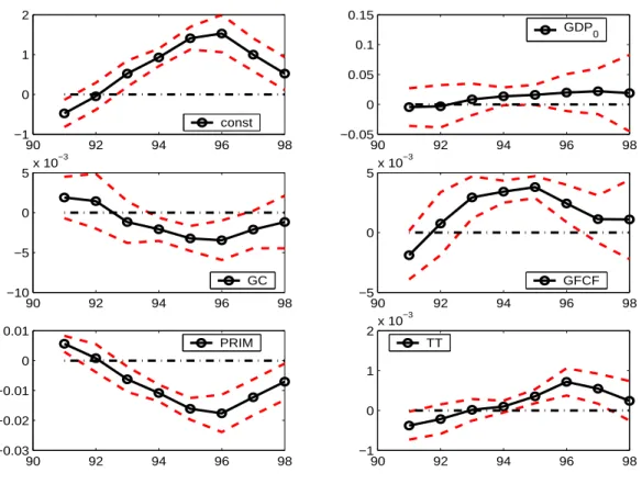
∆ logGDP_i =β₁+β₂logGDP_0,i+β₃GC_i+β₄GF CF_i+β₅P RIM_i+β₆T T_i+u_i (1) with ∆ logGDP denoting the average growth rate of real per capita GDP over the period investigated. GDP₀denotes initial real per capita GDP;GCdenotes the average government consumption share; GF CF denotes the average investment share; P RIM is an indicator of primary school education andT T denotes the average ratio of exports plus imports to GDP.

The error term is denoted by u and i is the country subscript. Equation (1) is estimated cross-sectionally for the periods 1991–2001 to 1998–2001, and the results are displayed in Figure 2. This figure displays therecursivecoefficients over the shrinking estimation intervals and the 95% confidence bounds. Of course the periods are extremely short for conducting growth analysis. Neoclassical growth theory predicts the following signs for the coefficients:

β₂<0,β₃ <0,β₄ >0,β₅>0 andβ₆>0. The first three of these sign restrictions correspond to the already discussed correlations and the latter two correspond to the positive effects of education and trade on growth. The results are quite clear: If the ‘correct’ sign prevails at

9The inclusion of further explanatory variables to study conditional correlations leads to conditional convergence concepts.

10Qualitatively similar results prevail throughout a whole variety of specifications.

(10)

90 92 94 96 98

−1 0 1 2

const

90 92 94 96 98

−0.05 0 0.05 0.1 0.15

GDP0

90 92 94 96 98

−10

−5 0 5x 10⁻³

GC

90 92 94 96 98

−5 0 5x 10⁻³

GFCF

90 92 94 96 98

−0.03

−0.02

−0.01 0 0.01

PRIM

90 92 94 96 98

−1 0 1 2x 10⁻³

TT

Figure 2: Recursive coefficient estimates (solid-circled lines) and 95% confidence intervals (dashed lines) for equation (1) estimated for the CEEC10 over shrinking estimation intervals.

The horizontal axis indicates the starting point of the period used for averaging, 1991–2001 to 1998–2001.

(11)

all, then only for a small patch of sub-periods. In particular, initial GDP is never significant, government consumption is negatively significant only when the equation is estimated over the periods 1994-2001 to 1996-2001. This is also approximately the set of periods which leads to a significantly positive coefficient for the investment share.¹¹ The figure also shows, with the caveat of very short time periods, that there is up to now no evidence that neoclassical growth theory is a good description of the growth performance of the CEEC10 group.

Two more issues in relation to Figure 2 deserve to be discussed. The first is the positive yet insignificant effect of initial GDP for the growth process. If initial GDP is accepted as an admittedly crude measure for initial conditions, then in sample of countries analyzed initial conditions do not significantly shape the growth process throughout the period. This is in line with the finding that initial conditions have rapidly declining importance for the transition process, see DeMelo et al. (1997), Havrylyshyn et al. (1998) or Berg et al. (1999).

The second issue is the effect of government consumption. The negative long-run correlation between government consumption and growth postulated by neoclassical growth theory cannot necessarily be expected to hold in the relatively short and turbulent transition period, where government consumption was an important policy variable to e.g. dampen the detrimental effects of the initial transformational recession. Thus, the absence of the negative long-run correlation that the growth literature is concerned with, also known as Wagner’s law, does not come as a big surprise. Furthermore, even in long-run growth studies authors find mixed evidence concerning this correlation, see Ram (1987) and Levine and Renelt (1992) for opposite results.

The results of this section imply that basing growth projections for the CEEC10 on growth or convergence equations estimated for the CEEC10, i.e. adirect approach, leads to projections of adivergentgrowth perspective for these economies. If one believes that this is not the most likely scenario, then an alternative approach that incorporates the EU accession of these countries and the likely subsequent convergence has to be sought. Note that a direct approach neglects in any case the effects of integration within the EU, even if it were based on a period of convergence within the CEEC10 themselves.

11Figure 7 in Appendix B displays the recursive coefficients for the same equation when estimated for 24 countries, the CEEC10 and the EU14 together. The figure shows that for that group of countries no coefficient is ever significant. Including dummies for the CEEC10 also fails to establish significant coefficients with theory consistent signs.

(12)

3 An Indirect Econometric Approach

The above discussion exemplifies again that projecting GDP growth of the CEEC10 based on the developments from 1991–2001 implies projecting the rather heterogeneous anddivergent growth process observed to date into the future. Therefore, such an approach generates growth scenarios that do not necessarily reflect the prospects that may materialize after successful completion of transition and in particular are bound to neglect the beneficial effects of integration within the EU.

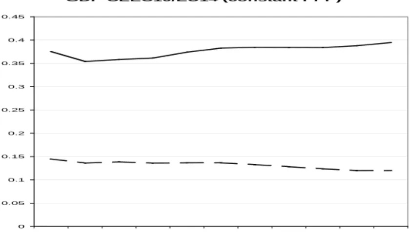
All the CEEC10 will be EU member states in the very near future and theireconomic size compared to the current European Union is small, see Figure 3. The solid line in Figure 3 displays the average real per capita GDP in the CEEC10 compared to the average real per capita GDP in the EU14, which has risen from about 35% in 1992 to almost 40% in 2001.

The dashed line displays the ratio of total real GDP of the CEEC10 to total real GDP of the EU14. This share actually declined from about 15% in 1992 to about 13% in 2001. This decline, despite growing relative per capita GDPs, stems from extraordinarily low population growth in the CEECs over the last decade. The average annual population growth rate in the CEEC10 over the period 1991–2001 is -0.15%, compared to 0.33% for the EU14. This compares with almost identical population growth rates in the period 1960–1990, with 0.68%

in the CEEC10 and 0.67% in the EU14. The smalleconomic sizeof the CEECs together with the continuedsystemic integration of these countries due to the upcoming EU enlargement, lead to an increased similarity of the economic and policy environment in the CEECs to the economic environment prevalent in the current EU member states. For instance the accession countries have to accept the EU legal code, as specified in theacquis communautaireand their markets for goods and factors will have to be open within the common market, at least after some transition period. Also, economic policy will have to be conducted in an increasingly similar way to how economic policy is conducted in incumbent member states.¹² Furthermore, about 70% of the CEEC10s exports are directed to the current European Union and the EU is the main source of foreign direct investment in the CEECs.

Thus, there have already been and there will be further important integration steps of the CEEC10 towards the EU along various dimensions, which will – unless a backlash occurs

12Note here again that for the new entrants later membership in the European Monetary Union is not optional but automatic after fulfillment of certain criteria. Thus, also the Maastricht criteria will impose relatively clear quantitative boundaries on the conduct of fiscal policy in the CEECs in the future.

(13)

GDP CEEC10/EU14 (constant PPP)

0 0.05 0.1 0.15 0.2 0.25 0.3 0.35 0.4 0.45

1991 1992 1993 1994 1995 1996 1997 1998 1999 2000 2001

Figure 3: Real per capita GDP in the CEEC10 relative to the real per capita GDP in the EU14 (solid line) and real GDP of the CEEC10 relative to real GDP of the EU14 (dashed line).

in some countries – lead to convergence of the CEEC10 as a group towards the current EU member states. Note here that Ben-David (1993) argues forcefully that historically EU integration contributed to convergence.¹³

Therefore an assessment of the growth prospects of the CEEC10 certainly has to take into account two main issues. First, the ongoing structural change due to economic transition. Second, the upcoming EU membership and the implied effects on integration and systemic convergence. To incorporate these two sets of effects, we base our growth projections on growth or convergence equations estimated for the current European Union members excluding Luxembourg, the EU14. These equations form the basis for growth projections or simulations, when combined with values for the independent variables taken from the CEECs or specified in scenarios. Such an indirect approach has been previously employed in the literature, see e.g. Fischer et al. (1998b). There are, however, two important differences of our study with respect to the existing studies. The first is the fact that we estimate growth equations for the EU and not for large world wide country sets with heterogeneous countries,

13More precisely, he analyzes the extent and timing ofσ-convergence among the founding countries of the European Community and the reduction of trade barriers and tariffs between the countries. He finds a close correspondence between measures that decrease barriers to trade and reductions in the standard deviation of log per capita GDP. See also Wagner and Hlouskova (2002) for an analysis ofσ-convergence in the CEECs and the EU.

(14)

IRL

GBR SWE PRT ESP

ITA NLD GRC

GER FRA FIN

DNK BEL AUT

0%

1%

2%

3%

4%

5%

8 8.2 8.4 8.6 8.8 9 9.2 9.4 9.6

IRL

GBR SWE

ESP PRT

NLD

ITA GRC

GER FRA

FIN

DNK BEL

AUT

0%

1%

2%

3%

4%

5%

17 19 21 23 25 27 29

IRL

GBR SWE

ESP PRT

NLD ITA

GRC

GER FRA FIN

DNK BEL AUT

0%

1%

2%

3%

4%

5%

10 12 14 16 18 20 22 24 26

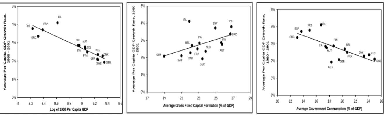
Figure 4: Correlations between the average real per capita GDP growth rate and the logarithm of 1960 real per capita GDP, the average investment share and the average government consumption share. The averages are computed over the period 1960–2001.

many of which are essentially unrelated to the CEECs. The second is that we try to assess the uncertainty in specifications for growth equations by specifying a variety of equations, 18 in total, and 7 scenarios. The specification of the equations follows the recommendation of Berg et al. (1999) to focus on specifications consistent with economic theory, because purely statistical approaches may lead to versatile and implausible conclusions. Thus, for each country we generate in total 126 growth rate projections. This allows for an uncertainty analysis by investigating the properties of the distributions of the projected growth rates.

Let us start by briefly discussing the growth process observed in the EU14. In Figure 4 we display the correlations between the real per capita GDP growth rate and the logarithm of initial real per capita GDP, the investment share and the government consumption share for the EU14 over the period 1960–2001. Strongly significant correlations of the expected signs are clearly visible, in contrast to Figure 1 for the CEECs. This illustrates again the well-studied convergence process amongst the current EU member states. Note that adding Luxembourg does not qualitatively change the picture and that similar pictures can also be drawn for sub-periods, e.g. for the four decades in the sample. Thus, estimating equations of the type (1) for the EU14 can be expected to lead to significant parameter estimates of the correct sign. See Table 2 for the set of 18 equations that form the basis for the growth projections in the following section. The growth equations are estimated by panel methods, compared to the usual cross-section regressions. The total sample period 1960–2001 is divided into the four sub-periods 1960–1969, 1970–1979, 1980–1989 and 1990-2001. Periods of about 10 years may be considered a fair compromise between taking long-run averages (to assess

(15)

long-run growth properties) and a sufficiently large number of observations (56 instead of 14 for a cross-sectional analysis). The equations are estimated pooled with seemingly unrelated regression (SUR) and heteroscedasticity between the different sub-periods is allowed for.

The variables, using the notation of Table 2, are the following and have mostly already been introduced in Section 2: ∆ logY, the averageannualgrowth rate of real per capita GDP (in constant PPP);GCdenotes the average share of government consumption in GDP;GF CF denotes the average share of investment (gross fixed capital formation including changes in inventories) in GDP; P RIM is an indicator of primary school education; T T is the average sum of exports and imports divided by GDP;Xdenotes the average share of exports in GDP and P OP G is the average population growth rate. A variety of the equations also contains dummies: D₁ is a dummy for the first period (1960–1969) which was a period of very rapid growth (annual real per capita GDP growth rate in the EU14 of 4.10%); a dummy for Ireland, D_IRL, which has an average growth rate over the period 1960–2001 of 4.11%; and a dummy for unified Germany, i.e. a dummy for Germany only for the period 1990–2001 only,D_GER. Taking average values of the independent variables is quite common in the literature. However, specifications that are based on the values of the independent variables over the first year are also commonly used, since these specifications may help to overcome potential endogeneity problems when using period averages (especially with respect to investment variables). We report four equations in Table 2 that are based on initial values for the independent variables, labelled with the suffix in. It turns out that in our case the results obtained from period average specifications and from initial period specifications are rather similar.

(16)

∆logGDPconstlogGDP0GCGFCFPRIMTTXPOPGD1DIRLDGERAdj.R2 (1)0.045-0.003-0.0890.0610.0100.0030.0130.639 (2.620)(-1.944)(-7.066)(4.975)(1.813)(2.508)(3.724) (1in)0.096-0.007-0.0840.0290.0040.0020.0110.616 (7.163)(-4.913)(-6.397)(2.845)(1.186)(1.464)(3.574) (2)0.066-0.005-0.0750.0560.0080.471 (3.808)(-3.055)(-6.153)(4.151)(1.338) (2in)0.107-0.008-0.0730.0310.0050.491 (8.025)(-5.873)(-6.620)(2.951)(1.261) (3)0.058-0.004-0.0740.0600.0090.0120.640 (3.336)(-2.790)(-6.142)(4.419)(1.436)(3.657) (4)0.061-0.003-0.0920.0510.0030.0120.635 (4.211)(-2.091)(-7.332)(4.222)(2.230)(3.661) (5)0.085-0.007-0.0460.066-0.1490.0130.470 (5.248)(-4.002)(-4.387)(4.819)(-1.065)(10.638) (6)0.074-0.006-0.0580.0650.0060.0040.2050.0150.463 (5.042)(-4.925)(-6.623)(5.939)(1.549)(4.865)(1.766)(13.280) (7)0.058-0.005-0.0640.0680.0080.0030.0120.449 (4.028)(-3.912)(-8.344)(7.059)(2.125)(4.308)(14.968) (8)0.049-0.004-0.0880.0610.0100.0060.0120.646 (2.922)(-2.330)(-6.933)(4.912)(1.818)(2.427)(3.690) (8in)0.098-0.007-0.0840.0290.0040.0040.0110.619 (7.483)(-5.229)(-6.469)(2.846)(1.136)(1.431)(3.562) (9)0.065-0.004-0.0910.0520.0050.0120.641 (4.589)(-2.440)(-7.246)(4.167)(2.151)(3.629) (9in)0.098-0.007-0.0850.0240.0040.0110.623 (7.869)(-4.752)(-6.730)(2.407)(3.622)(3.622) (10)0.064-0.005-0.0620.0670.0080.0060.0120.464 (4.282)(-4.286)(-7.867)(6.779)(2.061)(4.066)(14.525) (11)0.030-0.002-0.0750.0740.0150.004-0.4530.0030.293 (1.835)(-1.517)(-7.477)(6.892)(2.938)(2.339)(-4.401)(2.609) (12)0.030-0.003-0.0730.0770.0170.004-0.5250.0130.593 (2.089)(-1.779)(-6.223)(7.483)(3.174)(1.888)(-5.161)(4.350) (13)0.028-0.002-0.0740.0770.0170.002-0.5130.0130.600 (1.883)(-1.536)(-6.272)(7.483)(3.149)(1.933)(-5.095)(4.348) (14)0.043-0.003-0.0830.0640.0100.0030.0130.0030.621 (2.353)(-1.941)(-7.595)(5.221)(1.926)(2.858)(3.784)(3.041) able2:EstimationresultswithdependentvariableaveragerealpercapitaGDPgrowthrate.Theequationsareestimatedforthe Thefullsampleperiod1960–2001isseparatedinthefoursub-periods1960–1969,1970–1979,1980–1989and1990–2001.The aluesinbracketsareheteroscedasticitycorrected.Allvariablesaredescribedinthetext.Asuffixinindicatesthatintherespective thevaluesofindependentvariablesaretakenfromtheinitialperiod.

(17)

For most of the variables the expected signs of the coefficients have already been discussed in Section 2. Only exports and population growth need to be discussed. The reason for including exports in a growth equation is quite similar to including total trade, namely the positive effect of trade on growth. Including exports instead of total trade puts particular emphasis on so called export-led growth. Thus, a positive coefficient is expected for this variable. Increasing the population growth rate has a negative impact on per capita GDP growth, since with growing populationceteris paribusGDP has to be divided among a larger population. Hence a negative coefficient is expected. We have also experimented with other educational variables, like secondary school education indicators or the ratio of secondary to primary schooling, but of all education variables onlyP RIM appears to be statistically robust.

The results in Table 2 are all in line with the theoretical predictions, again confirming the fact that the growth (and convergence) process in the European Union can be satisfactorily described by neoclassical growth theory and growth equations derived therefrom. Averaging the results of the 18 equations, inserting the values of the last sub-period for the dependent variables and taking the population weights of 2001 leads to an implied growth rate of the EU14 of 2.14%. The actual growth rates for the EU14 over the periods 1970–1979, 1980–1989 and 1990–2001 are 2.83%, 1.96% and 1.74%. Similarly for the cohesion countries Greece, Portugal and Spain a growth rate of 2.65% is found from averaging over the equations. This compares with an actual growth rate of 2.37% over the period 1990–2001.

4 Growth and Convergence Scenarios

In this section the equations estimated in the previous section are used to generate growth rate projections for the CEEC10. To do so, assumptions concerning the explanatory variables have to be made. We choose scenarios for two variables, the government consumption share (GC) and the investment share (GF CF), and take actual values over the period 1991-2001 for the other variables. The assumed value for the population growth rate is 0. This is done since we assume that in the long-run the population growth differential that emerged between the EU14 and the CEEC10 over the period 1991-2001 is only temporary. Thus, in the long- run we assume the basically identical population growth rates to emerge again. Assuming a population growth rate of 0 keeps the population weights of the individual countries fixed at the same values as with identical growth rates for all countries, but allows us to avoid making

(18)

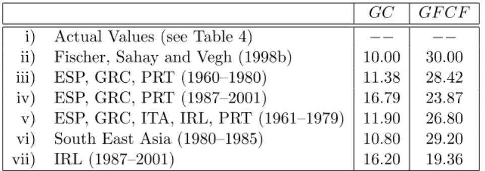
GC GF CF

i) Actual Values (see Table 4) −− −−

ii) Fischer, Sahay and Vegh (1998b) 10.00 30.00 iii) ESP, GRC, PRT (1960–1980) 11.38 28.42 iv) ESP, GRC, PRT (1987–2001) 16.79 23.87 v) ESP, GRC, ITA, IRL, PRT (1961–1979) 11.90 26.80 vi) South East Asia (1980–1985) 10.80 29.20

vii) IRL (1987–2001) 16.20 19.36

Table 3: Scenario values for the variables government consumption share and investment share. The values for scenario 1 are given in Table 4. South East Asia here denotes Indonesia, Japan, Malaysia, the Philippines and South Korea.

assumptions concerning population growth.¹⁴

We have chosen to base the scenarios on the two variablesGC and GF CF only, because these are among the most important variables for growth and are also directly policy-relevant variables. Another variable that might have been used for scenario analysis is total trade.

Taking average values over 1991–2001 for the growth scenarios means that the positive effects of trade are not fully reflected in the scenarios. Similarly, neglecting the dummies for the growth scenarios also contributes to scenarios that may be considered moderately optimistic.

A more substantial open issue is the fact that the effects of structural funds payments of the EU are not taken into account in the scenarios. The European Commission itself has estimates ranging from 0.4% to 1.2% additional annual growth due to EU payments. This interval can, if accepted as realistic, be added to the growth rate scenarios derived in this paper.¹⁵

The seven scenarios for the investment and government consumption shares we consider are displayed in Table 3. Scenario i) is based on the actual country specific values forGC and GF CF excluding early transition, see Table 4 for details including the periods chosen for averaging. All other scenarios employ identical values for GF CF and GC for all the CEEC10. Scenario ii) takes the values chosen by Fischer et al. (1998b) and is very similar to scenario vi), which is based on average values for South East Asian¹⁶ countries over the

14This assumption affects only 5 of the 18 equations.

15In Appendix B we report for completeness the resulting accelerated convergence time distributions and their characteristics for convergence to 80% of real per capita GDP in the EU14. Convergence to 80% of real per capita GDP in the EU14 is chosen, since this is the example displayed in detail later in this section. In Appendix B we display, paralleling the discussion of this section, also the mean and optimistic convergence times to a variety of other relative income levels.

16By South East Asia we denote here Indonesia, Japan, Malaysia, South Korea and the Philippines.

(19)

BGR CZE EST HUN LVA LTU POL ROM SVK SVN GC 15.14 20.20 22.62 10.92 20.24 20.78 17.72 12.95 20.40 20.55 GF CF 14.35 30.19 27.31 25.34 23.81 23.65 20.05 22.29 31.52 24.25 Period 94–01 92–01 94–01 92–01 94–01 95–01 92–01 93–01 93–01 93–01 Table 4: Country specific values for the government consumption share and the investment share used for scenario 1. The last row displays the periods used for averaging.

period 1980–1995. Thus, these two scenarios reflect the values observed in South East Asia over the period of rapid economic growth. Note that growth in South East Asia has been driven substantially by factor accumulation. Scenarios iii) to v) are based on values observed in peripheral current EU member states over various sub-periods. Finally, scenario vii) is based on the values observed for Ireland over the period 1987–2001. Note that contrary to the South East Asian experience the Irish growth performance has been achieved with a relatively low investment rate and a high government consumption share. The Irish example also shows that in order to understand the growth mechanisms of catching-up economies in detail, a more disaggregated analysis might be required. For instance it is important to disentangle investment into greenfield foreign direct investment (which often embodies latest technology) and domestic investment. Similarly, the effects of government consumption will be understood better in a more disaggregated analysis. These tasks, despite their importance, are beyond the scope of this paper, which solely provides an aggregative view on the growth prospects.

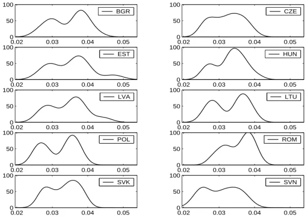
The 18 equations combined with the 7 scenarios lead to 126 growth rate projections for each country. We display this information in two ways. The first is graphical, where we show estimated densities for the growth rate distributions, and the second is numerical, where we display several characteristics of the distributions of growth rates (in Table 5).

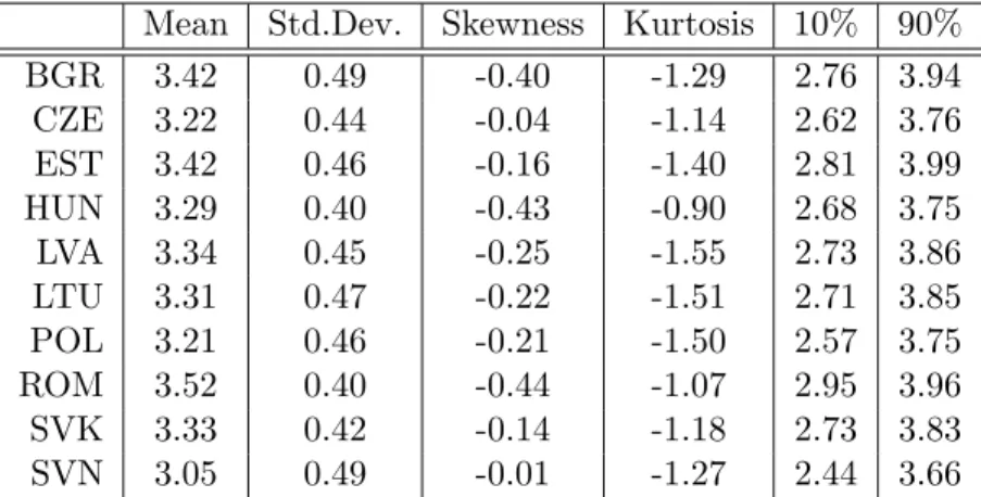
In Figure 5 the estimated densities of the projected growth rates are displayed. All density estimations performed in this paper are based on Gaussian kernels with bandwidths chosen according to Silverman’s rule of thumb. Most of the densities are bimodal with the larger probability weight surrounding the mode corresponding to the higher growth rate. The means range from 3.05% for Slovenia to 3.52% for Romania, see Table 5. The standard deviation is between 0.4 and 0.49, i.e. in the vicinity of half a percent growth per year, for all countries.

The table also displays skewness and kurtosis, both negative for all countries, as well as the first and ninth deciles of the distributions.

(20)

0.02 0.03 0.04 0.05 0

50 100

BGR

0.02 0.03 0.04 0.05

0 50 100

CZE

0.02 0.03 0.04 0.05

0 50 100

EST

0.02 0.03 0.04 0.05

0 50 100

HUN

0.02 0.03 0.04 0.05

0 50 100

LVA

0.02 0.03 0.04 0.05

0 50 100

LTU

0.02 0.03 0.04 0.05

0 50 100

POL

0.02 0.03 0.04 0.05

0 50 100

ROM

0.02 0.03 0.04 0.05

0 50 100

SVK

0.02 0.03 0.04 0.05

0 50 100

SVN

Figure 5: Density estimates of annual real per capita GDP growth rate projections. The countries are indicated in the boxes with the abbreviations used throughout the paper.

(21)

Mean Std.Dev. Skewness Kurtosis 10% 90%

BGR 3.42 0.49 -0.40 -1.29 2.76 3.94

CZE 3.22 0.44 -0.04 -1.14 2.62 3.76

EST 3.42 0.46 -0.16 -1.40 2.81 3.99

HUN 3.29 0.40 -0.43 -0.90 2.68 3.75

LVA 3.34 0.45 -0.25 -1.55 2.73 3.86

LTU 3.31 0.47 -0.22 -1.51 2.71 3.85

POL 3.21 0.46 -0.21 -1.50 2.57 3.75

ROM 3.52 0.40 -0.44 -1.07 2.95 3.96

SVK 3.33 0.42 -0.14 -1.18 2.73 3.83

SVN 3.05 0.49 -0.01 -1.27 2.44 3.66

Table 5: Moment and quantile characteristics of the distributions of the real per capita GDP growth rate projections.

The logic of basing the growth rate projections on linear growth equations estimated for the EU, implies that poorer CEE countries are ceteris paribus projected to grow faster. It is therefore stressed at this point that these growth projections should best be viewed as linear approximations to the nonlinear convergence process towards the EU14 income levels that the CEEC10 are likely to be experiencing. Perhaps more revealing than displaying the distributions of projected growth rates is a discussion of the implied convergence times. A discussion of convergence times requires the definition of the convergence level (e.g. 80% of income), the group of countries with respect to which convergence is measured (EU14, EU24 or C3) and also requires a growth assumption for the target country group. In this section we compute convergence times based on an assumed annual growth rate of real per capita GDP of 1.74% for the EU14 and 2.37% for the C3.¹⁷ Population weights are assumed constant at their 2001 levels. Note for completeness that these assumptions are sufficient to also compute convergence times with respect to the EU24.

Let us discuss in detail the convergence times distributions of the CEECs to a level of 80% of real per capita GDP of the EU14. Figure 6 displays the densities. Following from the bimodality of the growth rate distributions, the convergence time distributions are also bimodal, although to a lesser extent. Some of the densities are relatively flat, corresponding to large standard deviations, see Table 6 for some characteristics of the distributions. For instance for Romania, with the largest mean convergence time of 71.4 years and a standard

17In a separate appendix available upon requests we report similar results when the growth rate assumptions concerning the EU14 and the C3 are chosen to be the average values predicted from the equations, namely 2.14% and 2.65%. Obviously, the convergence times are larger then.