Temperature Assimilation into a Coastal Ocean-Biogeochemical
1
Model: Assessment of Weakly and Strongly-Coupled Data
2
Assimilation
3
Michael Goodliff,
1,3, Thorger Bruening
2, Fabian Schwichtenberg
2, Xin Li
2, Anja Lindenthal
2, Ina Lorkowski
2, Lars Nerger,
1∗1Alfred-Wegener-Institut Helmholtz-Zentrum f¨ur Polar- und Meeresforschung, Bremerhaven, Germany
2Bundesamt f¨ur Seeschifffahrt und Hydrographie, Hamburg, Germany
3now at Cooperative Institute for Research in the Atmosphere, Colorado State University, Fort Collins, USA
∗Corresponding author; phone: +49(471)4831-1558; E-mail: lars.nerger@awi.de
4
Satellite data of both physical properties as well as ocean colour can be assimilated into cou-
5
pled ocean-biogeochemical models with the aim to improve the model state. The physical ob-
6
servations like sea surface temperature usually have smaller errors than ocean colour, but it is
7
unclear how far they can also constrain the biogeochemical model variables. Here, the effect
8
of assimilating satellite sea surface temperature into the coastal ocean-biogeochemical model
9
HBM-ERGOM with nested model grids in the North and Baltic Seas is investigated. Weakly
10
and strongly-coupled assimilation is performed with an ensemble Kalman filter. For weakly-
11
coupled assimilation, the assimilation only directly influences the physical variables, while the
12
biogeochemical variables react only dynamically during the 12-hour forecast phases in between
13
the assimilation times. For strongly-coupled assimilation, both the physical and biogeochemical
14
variables are directly updated by the assimilation. The strongly-coupled assimilation is assessed
15
in two variants using the actual concentrations and the common approach to use the logarithm
16
of the concentrations of the biogeochemical fields. In this coastal domain, both the weakly and
17
strongly-coupled assimilation are stable, but only if the actual concentrations are used for the
18
strongly-coupled case. Compared to the weakly-coupled assimilation, the strongly-coupled as-
19
similation leads to stronger changes of the biogeochemical model fields. Validating the resulting
20
field estimates with independent in situ data shows only a clear improvement for the tempera-
21
ture and for oxygen concentrations, while no clear improvement of other biogeochemical fields
22
was found. The oxygen concentrations were more strongly improved with strongly-coupled than
23
weakly-coupled assimilation. The experiments further indicate that for the strongly-coupled as-
24
similation of physical observations the biogeochemical fields should be used with their actual
25
concentrations rather than the logarithmic concentrations.
26
Keywords
27
Data Assimilation; biogeochemistry; North Sea; Baltic Sea
28
1 Introduction
29
In recent years, ocean forecasting has become more common, e.g. with the European Copernicus Marine Environ-
30
ment Monitoring Service (CMEMS). In Germany, the Federal Maritime and Hydrographic Agency (BSH) operates
31
a forecasting system for the North and Baltic Seas based on the HIROMB-BOOS model (HBM, see, e.g.,Bruen-
32
ing et al.,2014). The national monitoring duties, e.g. to fulfil the European Marine Strategy Framework Directive
33
(MSFD) require monitoring the seas with regard to water quality and hence also for the ecosystem. Given that
34
in situ observations are sparse and hence insufficient for the monitoring, the extension of forecast models with an
35
ecosystem component is required. A coupled ocean-biogeochemical model, which simulates phytoplankton and
36
nutrients, can represent e.g. eutrophication, but can potentially also predict harmful algal blooms.
37
To initialise model forecasts, different observations can be assimilated. Satellite observations, e.g. of tem-
38
perature or sea level, are frequently available measurements of the sea surface. The assimilation of physical
39
observations to constrain the physical ocean model is common practice. However, it has been found that the as-
40
similation of these observations to constrain the physical ocean state can deteriorate the biogeochemical (BGC)
41
fields. For the North Atlantic,Berline et al.(2007) found that the assimilation of sea surface temperature (SST)
42
and sea surface height (SSH) data changed the mixed layer so that much higher vertical nutrient fluxes appeared
43
in the mid-latitudes and sub-tropics, which caused deteriorated phytoplankton concentrations. Also,While et al.
44
(2010) reported increased nutrients and in consequence overestimated primary production and chlorophyll concen-
45
trations in the subtropical gyres and at the equator. Similar increased upward flux of nutrients and corresponding
46
increased production was found byRaghukumar et al.(2015) in the California Current System. To correct for
47
spurious changes by the data assimilation, corrections to the nutrient fields have been proposed (While et al.,2010;
48
Shulman et al.,2013) whilePark et al.(2018) suggests to reduce the assimilation effect around the Equator.
49
There are also observations of the ocean colour, from which e.g. concentrations of chlorophyll or diffuse
50
attenuation rates are derived. In particular, chlorophyll concentrations have been used to directly influence the
51
BGC model state (e.g.Nerger and Gregg,2007,2008;Gregg,2008;Ciavatta et al.,2011;Ford et al.,2012;Ford
52
and Barciela,2017). However, the data errors are higher for chlorophyll than for physical quantities like SST.
53
Further, satellite chlorophyll observations have particularly high uncertainties in coastal waters, because the stan-
54
dard processing, like the ocean-colour algorithm byHu et al.(2012) commonly used in the processing of MODIS
55
data, is only valid for clear case-1 waters and the availability of data sets processed for the coastal regions is very
56
limited. Another data source on BGC quantities are in situ data, e.g. of nitrate. While these data are also available
57
below the surface, they are much more sparse than satellite data, which strongly limits their applicability for data
58
assimilation.
59
In coupled data assimilation, one can classify the data assimilation approach depending on which model
60
fields are influenced by which data type. The studies mentioned above performed so-called ’weakly-coupled’
61
assimilation, by assimilating observations of the ocean physics into the physical model component or assimilating
62
observations of BGC variables into the ecosystem component of the coupled model. A more sophisticated approach
63
is the ’strongly-coupled’ data assimilation. In this case, one uses cross-covariances between the physical and BGC
64
model components to let the assimilation algorithm utilise physical observations to directly update also BGC model
65
variables. Strongly-coupled data assimilation is challenging because it depends on the quality of the estimated
66
cross-covariances and requires that compatible assimilation methods are used in the different model components.
67
This appears to be a particular issue for the assimilation into coupled atmosphere-ocean models as the recent review
68
byPenny et al.(2017) shows.
69
Only a limited number of studies have so far considered the combined assimilation of physical and BGC
70
observations. However, while assimilating both physical and BGC observations, the published studies (Anderson
71
et al.,2000;Ourmi`eres et al.,2009;Song et al.,2016b,c;Mattern et al.,2017) all set the cross-covariances between
72
different variables to zero. Thus, in terminology of coupled data assimilation, only weakly-coupled data assimila-
73
tion was performed, in which the direct assimilation influence of the physical observation was only on the physical
74
model fields, while the BGC observations had only a direct influence on the modelled BGC concentrations. Only
75
during the subsequent model forecast, or in iterations of a variational minimisation method, the changed model
76
fields interacted. Nonetheless, the studies find that the combined weakly-coupled assimilation of physical and
77
BGC observations improved the overall consistency of the coupled model state.
78
Until now, strongly-coupled assimilation into a coupled ocean-BGC model was only studied by Yu et al.
79
(2018). The study used an idealised configuration of a channel with wind-induced upwelling and synthetically
80
generated observations, i.e. a twin experiment. Different combinations of weakly and strongly-coupled assim-
81
ilation assimilating either physical (SSH, SST and temperature profiles) or BGC data (surface chlorophyll and
82
nitrogen profiles) or assimilating both data types were conducted. The experiments showed that in this idealised
83
case, the cross-covariances between the physical and BGC model variables contain useful information that can be
84
used in the strongly-coupled assimilation.
85
In this study, the effect of strongly-coupled assimilation in a realistic ocean-BGC model is assessed. For this
86
purpose, the data assimilation is performed on the coastal coupled ocean-BGC model HBM-ERGOM configured
87
for the North and Baltic Seas using two nested meshes. An earlier model version of the physical circulation
88
model (BSHcmod,Dick et al.,2001;Kleine,2003) with a simpler model configuration without nesting was used
89
in previous studies (Losa et al.,2012,2014;Nerger et al.,2016) to assess the influence of SST assimilation. Only
90
satellite SST data is assimilated here and the effect of both weakly and strongly-coupled assimilation is assessed.
91
A particular focus is on the question whether the strongly-coupled assimilation of SST data, i.e. direct joint update
92
of both the physical and BGC model fields, improves the model state in this coastal setup.
93
A further aspect examined here is the different effect when treating the BGC model fields in the assimilation
94
using the actual concentrations or the logarithm of them. Based on the fact that the chlorophyll concentrations
95
can be well described as log-normally distributed (Campbell,1995), many studies employing ensemble Kalman
96
filters (e.g.Nerger and Gregg,2007,2008;Ciavatta et al.,2011;Pradhan et al.,2019) or optimal interpolation
97
(Ford et al.,2012) have applied the data assimilation to the logarithm of the concentrations or by applying a so-
98
called anamorphosis transformation (Doron et al., 2011). For the BGC assimilation with variational methods,
99
Song et al.(2016a) have developed a method to treat lognormal concentration distributions. On the other hand,
100
the actual concentrations have been used by other studies applying ensemble Kalman filters (e.g.Carmillet et al.,
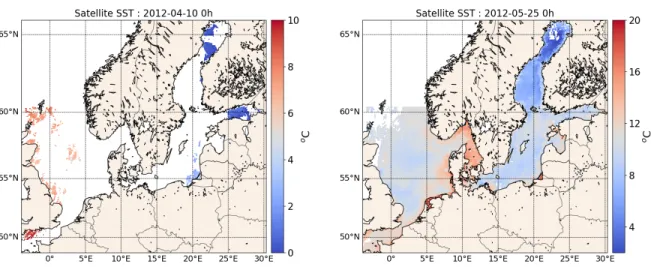
101
2001;Natvik and Evensen,2003;Mattern et al.,2010;Yu et al.,2018) and 3-dimensional variational assimilation
102
(Teruzzi et al.,2014). The latter study also discusses that actual concentrations were used because only then the
103
typical structure of vertical chlorophyll profiles was preserved. In this study, both cases of actual and logarithmic
104
concentrations are examined.
105
This study is structured as follows: Section2describes the coupled model HBM-ERGOM. The data assim-
106
ilation methodology and the observations assimilated and used for validation are described in Sec.3 while Sec.
107
4describes the setup of the data assimilation experiments. The assimilation effect is assessed in Sec.5for using
108
actual biogeochemical concentrations and in Sec.6for the case of the logarithmic treatment of the biogeochemical
109
variables. The results are discussed in Sec.7while conclusions are drawn in Sec.8.
110
2 HBM-ERGOM model
111
The model used here is the HIROMB-BOOS-Model (HBM) coupled to the BGC model ERGOM. HBM is currently
112
used operationally, without data assimilation, by the BSH in a similar configuration as used here. The coupled
113
HBM-ERGOM configuration is currently used pre-operationally at the BSH.
114
HBM is a three-dimensional hydrostatic circulation model using the primitive equations. It uses spherical
115
horizontal and generalised vertical coordinates (Kleine,2003). The model domain extends from 4◦W to 30.5◦E
116
and from 48.5◦N to 60.5◦N in the North Sea and to 66◦N in the Baltic Sea. A nested configuration of the model
117
is used with two domains shown in Fig.1. The coarser grid covers the entire North Sea and Baltic Sea. It has
118
horizontal grid spacing of about 5 km (5’ in longitude and 3’ in latitude) and 36 vertical layers. In the region of
119
German territorial waters in the North Sea and Baltic Sea, a finer grid with a horizontal resolution of about 900 m
120
(50” in longitude and 30” in latitude) and 25 vertical layers is nested into the coarse grid using a 2-way nesting.
121
In the North Sea, the model configuration has a northern open boundary in the coarse mesh, which is closed
122
with a sponge layer. Within this layer, the temperature and salinity are restored towards monthly mean climatolog-
123
ical values (Janssen et al.,1999). A similar sponge region is included at the entrance to the English Channel. A
124
two-dimensional model for the North East Atlantic, which is run separately by the BSH, provides information on
125
external surges at the open boundaries. Tidal forcing is implemented using 14 tidal constituents and flooding and
126
drying of tidal flats is applied (Bruening et al.,2014). The atmospheric forcing at the surface is based on meteo-
127
rological forecast data provided by the German Weather Service (DWD). River runoff is prescribed as freshwater
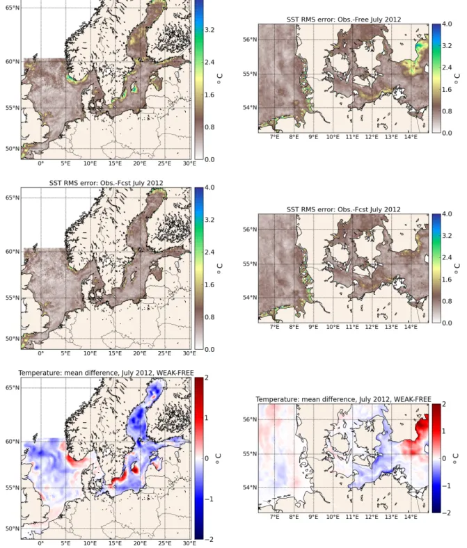
128
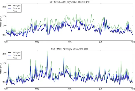
fluxes at the boundaries opened in the regions of main rivers. Further, HBM includes a sea-ice model component
129
that describes sea ice thermodynamics and incorporates Hibler-type dynamics (Hibler,1979).
130
The BGC model ERGOM was originally developed byNeumann (2000) for the Baltic Sea and upgraded
131
later byMaar et al.(2011) for the ecosystems in the North and Baltic Seas. ERGOM simulates the BGC cycling
132
in the coastal seas using three phytoplankton groups (Cyanobacteria, Flagellates, Diatoms), two zooplankton size
133
groups, four nutrient groups (nitrate, ammonium, phosphate, and silicate), two detritus groups (N-Detritus and
134
Si-Detritus), oxygen and labile dissolved organic nitrogen in the water column (lDON,Neumann et al.,2015). The
135
phytoplankton and zooplankton groups are expressed in nitrogen concentrations. The chlorophyll-a concentration
136
and the Secchi depth are computed diagnostically (Doron et al.,2013;Neumann et al.,2015). Riverine load inflow
137
of nutrients was derived from climatological data for major rivers. The boundary conditions for the BGC state
138
variables are from the World Ocean Atlas (WOA05) as described byMaar et al.(2011). ERGOM is coupled
139
one-way to HBM so that the physical fields influence the biogeochemistry, which itself does not influence the
140
physics.
141
3 Data Assimilation
142
The data assimilation is performed using the ensemble-based Error-Subspace Transform Kalman filter (ESTKF
143
Nerger et al.,2012b) provided by the Parallel Data Assimilation Framework (PDAF,Nerger et al.(2005);Nerger
144
and Hiller(2013)), which are described in this section.
145
3.1 Parallel Data Assimilation Framework
146
The Parallel Data Assimilation Framework (PDAF,Nerger et al.(2005);Nerger and Hiller(2013), http://pdaf.awi.de)
147
is an open-source software environment for ensemble data assimilation. It simplifies the implementation of the data
148
assimilation system with existing numerical models by providing support to modify the model to compute ensem-
149
ble forecasts and by providing fully implemented ensemble data assimilation methods. For the data assimilation,
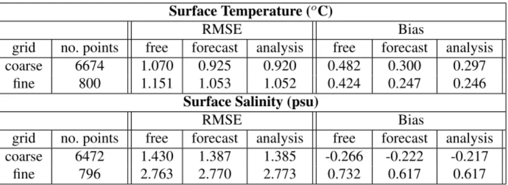
150
the model code is augmented by subroutine calls to PDAF. This changes the parallelisation of the model, so that it
151
can simulate an ensemble of model states, which are then used in the analysis step of the data assimilation, where
152
the observational information are incorporated into the model.
153
3.2 Error-Subspace Transform Kalman Filter
154
The data assimilation method used here is the Error-Subspace Transform Kalman Filter (ESTKF,Nerger et al.,
155
2012a). The ESTKF is an efficient variant of the ensemble Kalman filter, which uses an ensemble ofNemodel
156
states to represent the state estimate, as the ensemble mean, and its uncertainty by the ensemble spread. For an
157
overview of different filter methods, seeVetra-Carvalho et al.(2018).
158
The ESTKF performs a sequential assimilation by alternating forecast phases and analysis steps. In the
159
forecast phase, all model states in the ensemble are integrated by the model until the time when observations
160
become available. Then, the analysis step is computed in which the observational information is assimilated into
161
the model states.
162
Compared to the classical ensemble Kalman filter (EnKFEvensen,1994;Burgers et al.,1998), the analysis
163
step of the ESTKF is a particularly efficient formulation because it takes into account that the number of the
164
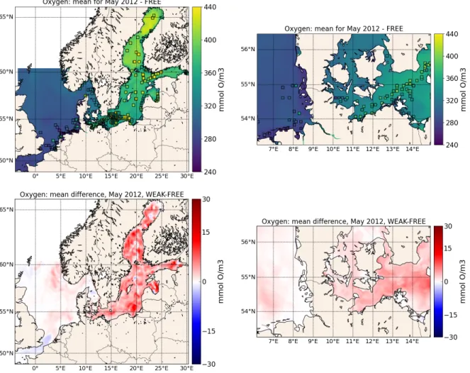
degrees of freedom for the analysis update is given byNe−1, while the EnKF computes the update according
165
to the usually much higher number of observations (seeNerger et al.(2005) for a comparison of the EnKF with
166
the SEIK filter, which has the same efficiency as the ESTKF). Mathematically, the ensemble describes the degrees
167
of freedom by spanning an error-subspace of dimensionNe−1, which motivates the name of the filter method.
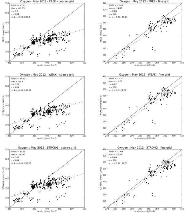
168
In the analysis step, the ESTKF uses ensemble-sampled error covariances of the model forecast, the observation
169
error, and the observational values to estimate the true state of the system. The ESTKF does this as follows by
170
computing transformation weights. LetXkdenote an ensemble matrix at timekin which each of theNecolumns
171
represents one model state. The transformation of the forecast ensemble,Xfk into the analysis ensemble,Xak is
172
given by
173
Xak = ¯Xfk+XfkWk (1)
where the overbar denotes the ensemble mean andWkis a transformation matrix of sizeNe×Ne. Given that the
174
degrees of freedom given by the ensemble areNe−1, this transformation matrix is calculated in an error-subspace
175
of dimensionNe−1at timek. Below, we omit the time indexk, as all calculations of the analysis step are at
176
this time. The transformation matrix is computed as follows. First, the ensemble states are projected onto the error
177
subspace by
178
L=XfT, (2)
whereTis a projection matrix of sizeNe×(Ne−1)given by the set of equations
179
Tj,i=
1−N1
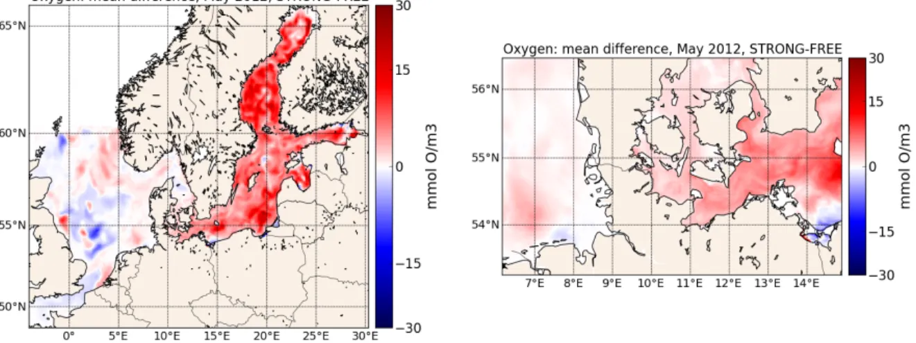
e
1
√1
Ne+1, fori=j,j < Ne
−N1
e
1
√1
Ne+1, fori6=j,j < Ne
−√1
Ne, forj=Ne.
(3)
Now the matrix
180
A−1=ρ(Ne−1)I+ (HXfT)TR−1(HXfT) (4)
of size(Ne−1)×(Ne−1)is computed. Here,ρis the so-called forgetting factor, which is chosen as0≤ρ≤1
181
and inflates the ensemble variance to stabilise the filter process.Iis the identity matrix andHis the observation
182
operator which computes the model equivalent to the observations so that one can writey=Hxf+ηwhereyis
183
the observation vector of sizeNy,xfis a forecast state vector andηis the observation error, which is assumed to
184
be Gaussian with observation error covariance matrixR.
185
The weight matrixWin Eq. (1) is now computed as the sum of two terms
186
W= ¯W+ ˜W. (5)
Here,W¯ contains in each column the vector
187
¯
w=TA(HXfT)TR−1(y−Hx¯f) (6)
which performs the transformation of the ensemble mean, while the ensemble perturbations are transformed by
188
W˜ =p
Ne−1TA1/2TT. (7)
HereA1/2 =US1/2UT is the symmetric square root ofAcomputed from the eigenvalue decompositionA =
189
USUT.
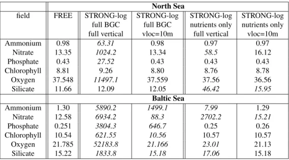
190
The degrees of freedom provided by the ensemble are too small to successfully assimilate the large number
191
of satellite observations. Due to this, the ESKTF is applied here with a localised analysis as for the LSEIK filter
192
(Nerger et al.,2006). Namely, the model state of each vertical column of the model grid is updated separately
193
taking only observations into account that lie within a specified influence radius around the water column. Further,
194
the observations are weighted according to their distance to reduce the influence of remote observations and to
195
generate a smooth analysis field. For the weighting, the inverse observation error covariance matrix in Eq. (4) is
196
multiplied element-by-element with a diagonal matrix constructed using the regulated localization ofNerger et al.
197
(2012a) with a correlation function given by the fifth-order polynomial ofGaspari and Cohn(1999). This function
198
mimics a Gaussian function and varies between one at zero distance and zero at the distance of the influence radius.
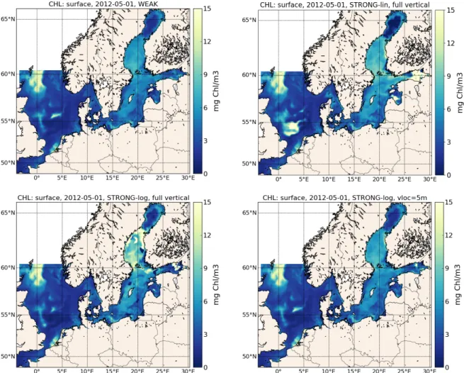
199
Since the model uses nested grids with different resolutions, one has to adapt the localisation. Here, the
200
influence radius is chosen according to the location of the observation, as is depicted in Fig.2. Thus, an observation
201
located in the coarse grid is only taken into account for model grid points within the radiusrg, while an observation
202
located in the fine grid is only taking into account within the radiusrf. Accordingly, the analysis update of a water
203
column on the coarse grid also takes into account observations on the fine grid (vice versa for the update on the
204
fine grid) if the grid point is sufficiently close to the fine grid. This ensures a smooth transition of the analysis field
205
across the boundary of both grids.
206
3.3 Observations
207
In the experiments, satellite observations of the sea surface temperature are assimilated. These are measured with
208
the Advanced Very High Resolution Radiometer (AVHRR) aboard polar orbiting NOAA satellites and processed
209
by the BSH. Composites over 12 hours are used which are interpolated onto the two nested model grids. The
210
composites use the satellite information over the 12-hour time window before the analysis step. Given that the
211
radiometer provides only data for clear-sky conditions, the data coverage can vary significantly as shown in Fig.
212
3. This is particularly noticeable in the rather small fine grid region for the German coastal regions, where even
213
12-hour time windows with zero coverage can exist.
214
For the validation of the assimilation results, a data set of in situ data is used. The data set includes data from
215
the International Council for the Exploration of the Sea (ICES Dataset on Ocean Hydrography. The International
216
Council for the Exploration of the Sea, Copenhagen. 2016) and the German Oceanographic Data Center (DOD,
217
http://seadata.bsh.de/csr/retrieve/dod index.html) operated by the BSH. Apart from water temperature and salinity,
218
the data set also includes measured concentrations of oxygen, nitrate, ammonium, phosphate, silicate, and chloro-
219
phyll, which can be used to assess the corresponding concentrations in the ERGOM model. The validation of the
220
assimilation experiments will focus on the surface and will be conducted for both the fine and coarse model grids.
221
4 Experimental Setup
222
The assimilation experiments are conducted over the time period from April to July 2012 with an analysis update
223
after each 12 h. An ensemble of 40 model states is used. The initial physical ocean state (i.e. ensemble mean)
224
is provided by the operational run of the HBM model at the BSH. The BGC model state was initialised on 1st
225
November 2011 using for the Baltic Sea an initial state provided by the Danish Technical University (generated
226
by the model ofMaar et al.(2011) by M. Maar, personal communication) and for the North Sea an initial state
227
generated by the model ofLorkowski et al.(2012). The ensemble perturbations were computed using 2nd-order
228
exact sampling (Pham et al.,1998) using the variability of the model state in a forecast run of the HBM-ERGOM
229
model for April 2012.
230
The state vector for the assimilation jointly includes the model fields on both nested model grids (similar to
231
Barth et al.,2007) and consists of physical and BGC parts on both nested model grids. For the physical part the state
232
vector includes the SSH and the 3-dimensional temperature, salinity, and horizontal velocities. For ERGOM, all 13
233
prognostic pelagic and 2 benthic variables as well as the Secchi depth and chlorophyll concentration are included
234
in the state vector. The two latter diagnostic variables are, however, only included to access their ensemble values,
235
but they are not directly updated by the analysis step of the LESTKF. For the localisation of the analysis step an
236
influence radius for the observations of 50 km is used for the coarse grid, while 9 km are used for the fine grid.
237
An inflation of the ensemble variance with a forgetting factor ofρ= 0.95is used. For the assimilation of the SST
238
observations, an observation error standard deviation of 0.8oC is assumed as inLosa et al.(2014) for both model
239
grids.
240
Two assimilation experiments are performed to assess the different effects of the weakly and strongly-coupled
241
assimilation. The experiment WEAK assimilates the SST observations so that only the physical model fields in the
242
state vector are directly updated. The BGC model fields react only dynamically to the changed physical conditions
243
during the next forecast phase of 12 hours. In contrast, in the experiment STRONG both the physical as well as
244
BGC model fields are directly updated. Thus, the strongly-coupled assimilation uses the multivariate ensemble-
245
estimated cross-covariances between the SST and the BGC variables to compute an update of the biogeochemistry.
246
Further, the experiment FREE was performed in which the ensemble was integrated without assimilating observa-
247
tions.
248
The experiment STRONG is performed in two variants. STRONG-lin performs the assimilation using the
249
actual concentrations of the BGC variables. In this case, the statistical update computed by the LESTKF can
250
result in negative concentrations. As inYu et al.(2018), these values were reset to zero, but occurred only in a
251
few cases in the experiments. The experiment STRONG-log performs the assimilation using the logarithm of the
252
concentrations.
253
The experiments allow us to assess whether the cross-covariances between the SST and the BGC model fields
254
are sufficiently well estimated to result in an improvement of the BGC fields. For this, the root mean square error
255
(RMSE) and the mean error (bias) between the state estimate from each data assimilation experiment with regard to
256
the in situ validation data are computed. To assess the impact of the SST data on the modelled surface temperature
257
and salinity we also compute the RMSE with regard to the assimilated data as well as RMSE and bias with regard
258
to independent in situ data of temperature and salinity.
259
5 Results
260
To analyse the assimilation results, first the influence on the surface temperature and salinity are assessed. Then,
261
the effect of the weakly-coupled assimilation on the biogeochemical model fields is examined, and finally, the
262
effect of the strongly-coupled assimilation is assessed.
263
5.1 Influence of the assimilation on surface temperature and salinity
264
The effect of assimilating satellite SST data on the physical ocean state was already discussed byLosa et al.(2012)
265
andLosa et al.(2014), so no detailed analysis is performed here. Figure 4shows the RMSE with regard to the
266
assimilated SST observations for the analysis and forecast fields each 12 hours as a time series for both model
267
grids. For the forecasts, the RMSE is computed with observations that have not yet been assimilated. Given that
268
the coverage of the SST observations varies in between the analysis times, the observations at the forecast time
269
are partly independent, while they are not independent for the analysis. Nonetheless, the values of the RMSE for
270
the forecast and analysis are very similar. Since HBM-ERGOM uses a one-way coupling between the physical
271
and biogeochemical models, the physical model fields are identical in the experiments WEAK and STRONG. The
272
assimilation of SST data pulls the SST in the model toward the observations while accounting for the uncertainty
273
in both the model state and the observations. Further, through the covariances estimated by the ensemble, the
274
observational information is interpolated spatially and unobserved model fields are modified. For the coarse grid
275
(upper panel) the RMSE of the forecast and analysis is clearly reduced compared to the free run. For the fine grid
276
(lower panel), the RMSE is also reduced, but the fluctuations of the errors between the different analysis times
277
are larger and the overall error-reduction is smaller. Namely, the average RMSE is reduced in the forecast by
278
0.21oC (from 1.02oC for the free run to 0.81oC) on the coarse grid while the reduction is 0.14oC (from 0.89oC
279
to 0.75oC) on the fine grid. Nonetheless, on the fine grid the error is lower on average compared to the coarse
280
grid. The strong variations of the RMSE, which are particularly visible for the fine model grid, are mainly due
281
to the varying data coverage in between the analysis times. Both the number of observations and the observation
282
locations varied strongly, so that the computation of the RMSE covers different regions and a strongly varying
283
number of comparison points, which leads to sampling errors. For example, on May 10th at 12h, when the highest
284
RMSE occurs on the fine grid, only 893 grid points out of 124000 overall surface grid points were observed. Just
285
before, at 0h on May 10th, there were 12275 observed grid points and at 0h on May 11th, 2464 observations were
286
available. Likewise on May 11 at 0h there is a very low number of only about 2000 observed grid points in the
287
coarse grid and a particularly small RMSE. Apart from this effect, the data assimilation process of alternating
288
analyses and forecasts induces a gradual modification of the ocean state over time as is visible from the small
289
difference between the RMSE in the forecasts and analyses, but larger RMSE in the free run. Accordingly, the
290
RMSE of the forecast or analysis at a certain time, depends on the observations that have been assimilated before.
291
Overall, the variability of the RMSE is mainly caused by the coverage of the observations and less by specific
292
oceanographic events.
293
While the spatially averaged RMSE of the forecasts shows only small reductions by the data assimilation up
294
to 0.21oC (and 0.24oC for the analysis states), the assimilation influence is locally much larger. Fig.5shows the
295
effect of the assimilation as an average over July 2012. The RMSE in the FREE run (upper row) is mainly below
296
0.8oC in both grids, but it is larger in the western side of the English channel, in the region of the Norwegian
297
trench, along the south-eastern coast of Sweden, the Gulf of Bothnia, and at the southern coast of Finland (see Fig.
298
1for geographic information). Locally, the RMSE exceeds 4oC. The data assimilation strongly reduces these high
299
errors almost everywhere except in the far northern end of the Baltic Sea and in the English channel (middle row).
300
In the fine grid, the error reductions are particularly visible at the southern coast of Sweden and along the German
301
coast of the Baltic Sea. The bottom row of Fig.5shows the actual change in the temperature. In most regions of
302
the model domain the assimilation has reduced the temperature. However, east of the islands ¨Oland and Gotland,
303
the temperature is increased up to 2oC. Here, upwelling of cold water was present in the free model run, which is
304
not present in the observations. The assimilation of the SST data increases the SST in the full water column hence
305
decreasing the RMSE. Overall, the error reductions are similar to those described byLosa et al.(2012) andLosa
306
et al.(2014) where SST data with a similar model was used without a refined nested grid. The comparison with the
307
assimilated observations shows that the assimilation system is successful in incorporating the observational SST
308
data.
309
Table1shows the RMSEs computed with regard to the in situ observations of SST over the full period from
310
April to July 2012. The number of in situ data is overall low with 6674 points on the coarse grid and 800 points
311
on the fine grid. On the coarse grid, the assimilation reduces the RMSE from 1.07oC in the FREE run to 0.92oC
312
in the analysis. The forecast RMSE is only slightly larger with 0.925oC. The RMSE of the FREE run is 1.15oC
313
and hence larger than on the coarse grid. This is in contrast to the RMSE with regard to the assimilated satellite
314
observations, where the RMSE on the fine grid is lower than on the coarse grid. The RMSE is reduced by the data
315
assimilation to 1.05oC. Overall the reduction of the RMSE is lower for the in situ data than the assimilated SST
316
observations. The assimilation also reduces the warm bias of the model SST in both model grids. On the coarse
317
grid, the bias is reduced by 62%, while it is reduced by 58% on the fine grid. So, the reduction of the bias is overall
318
larger than that of the RMSE.
319
The lower part of Table1shows the RMSE for surface salinity. Overall the changes to the salinity RMSE are
320
very small. The changes are due to the direct update of the salinity field through the cross-covariances between
321
the temperature and salinity, but also due to the fact that the assimilation also influences the velocities. The
322
assimilation reduces the error on the coarse grid from 1.43 PSU to 1.39 PSU in the analysis. On the fine grid, the
323
RMSE of the salinity is slightly increased by about 0.4% by the assimilation. While the changes in the RMSE
324
and bias are statistically significant for the coarse grid only the change in bias is significant for the fine grid (at
325
95% probability according to a paired t-test). Locally the largest changes happen in the transition zone between
326
the salty North Sea (around 35 PSU) and the fresh Baltic Sea (5 to 8 PSU), i.e. the Danish Straits in the fine grid
327
and the Skagerrak and Kattegat in the coarse grid. The assimilation also reduces the amount of bias by about 8%.
328
The model underestimates the salinity in the coarse grid, while it overestimates the salinity in the fine grid.
329
5.2 Weakly-coupled assimilation effect on the biogeochemical model fields
330
In the weakly-coupled data assimilation, only the physical model fields are directly updated by the LESTKF in
331
the analysis step. The BGC model fields then react dynamically on the changed physical conditions during the
332
following forecast phase. Table2shows the RMSE and bias computed with regard to the in situ data for 6 BGC
333
variables. The changes are largest for oxygen with a reduction of the RMSE by 3.5% and bias by 17% on the
334
coarse grid and a reduction of the bias by 64% on the fine grid. These changes are statistically significant at 95%
335
probability using a paired t-test. Changes to other variables are generally smaller.
336
To get more insight into the changes to the biogeochemistry which are induced by the data assimilation, we
337
examine the surface oxygen during the month of May 2012. Figure6shows monthly averaged oxygen concentra-
338
tion for the experiment FREE for both model grids. The in situ data values are plotted on top of the model fields.
339
In the Baltic Sea, but also in the German Bight in the North Sea, the model mainly underestimates the oxygen
340
concentration.
341
The bottom row of Fig.6shows the difference between the oxygen concentrations from the WEAK and FREE
342
experiments averaged over May 2012. The dynamic reaction of the model on the assimilation is to increase the
343
oxygen concentration by up to 18 mmol/m3in the Baltic Sea, which reduces the model bias. The dynamic reaction
344
on the assimilation is much smaller in the North Sea with increases and decreases up to 5 mmol/m3. Fig.7shows
345
the comparison between the model concentrations and the in situ data as scatter plots. Consistent with Fig.6, the
346
main influence of the assimilation is to increase concentrations that are above 340 mmol/m3 in the experiment
347
FREE. For the group of data points at about 350 mmol/m3in the coarse grid this lead to a slight overestimation of
348
oxygen. Since also larger concentrations that are generally too low in the model are further increased the overall
349
assimilation effect is positive. Thus, the assimilation reduces the RMSE and the amount of bias with statistically
350
significance (at 95% probability). However, the correlation between the model and the situ data remains essentially
351
unchanged. The overall assimilation effect is similar in April and June, while it is lower for July.
352
5.3 Strongly-coupled assimilation effect on the biogeochemical model fields
353
In the strongly-coupled data assimilation experiments STRONG-lin and STRONG-log, all BGC model fields
354
are directly updated, together with the physical fields, by the LESTKF utilising the ensemble-estimated cross-
355
covariances between the SST and the BGC fields. Thus, one expects a more directed and larger influence of the
356
assimilation. If some BGC model field is not correlated with SST, the ensemble represents this relation (up to sam-
357
pling error in the ensemble). In this section, the assimilation effect for the experiment STRONG-lin is examined,
358
i.e. for the case that actual concentrations are used in the LESTKF. The experiment STRONG-log is discussed in
359
Sec.6.
360
Table3shows the RMSE and bias with regard to the in situ data for the experiment STRONG-lin. The change
361
in the RMSEs is slightly larger than for the weakly-coupled assimilation. The largest change happens for oxygen
362
on the coarse grid where the RMSE is reduced by 4.7% in the experiment STRONG-lin, while it was only reduced
363
by 3.5% in WEAK. Further, the amount of bias is now reduced by 24% compared to 17% in WEAK. On the fine
364
grid the amount of bias is also more strongly decreased (by 89%), while the RMSE is now increased by 1.9%. The
365
changes to the other fields are still small. Noticeable is a reduction of the bias for chlorophyll on both grids and for
366
Silicate on the fine grid. The RMSE for chlorophyll was essentially unchanged in WEAK, but is increased slightly
367
in STRONG-lin. Actually, in the eastern Gulf of Finland the chlorophyll concentration was unrealistically high
368
during the first half of May in STRONG-lin. This effect will be further discussed in Sec.7. Further, the biases for
369
nitrate and phosphate are increased in STRONG-lin in the coarse grid, while they were marginally decreased in
370
WEAK.
371
Figure8shows the change in the oxygen field averaged over May 2012. Compared to the weakly-coupled
372
assimilation, the strongly-coupled assimilation results in larger changes up to 24 mmol/m3. Further the strongly-
373
coupled assimilation leads to larger changes in the North Sea up to 10 mmol/m3. The bottom row of Fig.7shows
374
the comparison between the model and in situ data for May 2012. The strongly-coupled assimilation further
375
increases concentrations that were above 340 mmol/m3 in the experiment FREE compared to the experiment
376
WEAK, which reduces both RMSE and bias on both grids for this month.
377
Several studies (e.g.Shulman et al.,2013; While et al.,2010;Yu et al.,2018) applied the assimilation of
378
physical observations so that in the BGC model only nutrients are updated, instead of all BGC model fields. We
379
performed an alternative experiment in which the phytoplankton, zooplankton, and detritus were excluded from the
380
assimilation update. The assimilation influence on the RMSE and bias with regard to the in situ data is summarised
381
in the right columns of table3. With this update variant, the RMSE of nitrate, chlorophyll, oxygen, and silicate
382
are reduced in both model grids by up to 2% compared to the case when all fields are updated. However, the
383
amount of bias increased in particular for oxygen and chlorophyll concentrations with increases of 6% and 29%,
384
respectively. Note that here chlorophyll is particular because it is computed from the phytoplankton, which is not
385
directly updated by the data assimilation in this experiments. In this experiment, the high concentrations in the
386
Gulf of Finland were not present.
387
6 Assimilation using logarithmic concentrations
388
Above, the strongly-coupled assimilation was applied in the experiment STRONG-lin using the actual concentra-
389
tion values of the BGC fields in the state vector. As discussed in the introduction, chlorophyll concentrations can
390
be well described as log-normally distributed (Campbell,1995) which motivated many assimilation studies to use
391
the logarithm of the concentrations in the state vector. The analysis step in the Kalman filter assumes normal error
392
distributions for optimality and taking the logarithm of a log-normally distributed field results in a normal distri-
393
bution. Likewise, this transformation is then applied to other BGC variables. While using actual concentrations
394
appears to be statistically inconsistent with the assumptions of the Kalman filter, the studies using actual concentra-
395
tions in the assimilation were also successful. This can be mainly explained by the fact that the assimilation using
396
actual concentrations still results in corrections of the correct sign. However, the size of the correction will be dif-
397
ferent because normal distribution is symmetric while the log-normal distribution is skewed. Using the logarithm
398
will typically lead to a tendency to more strongly increase concentrations. According to our experience, using
399
the logarithm also leads overall to larger changes to the concentrations and a more sensitive assimilation system
400
in particular for non-observed parts of the model fields like below the ocean surface. Due to this,Pradhan et al.
401
(2019) introduced a vertical localisation to stabilise the assimilation update of subsurface variables. In this vertical
402
localisation, the assimilation increment computed for the full water column is linearly reduced as a function of
403
depth until it reaches zero at a prescribed depth (100m inPradhan et al.(2019)).
404
In Sec.5.3, we found that the strongly-coupled assimilation applied with the actual concentrations improved
405
the oxygen concentrations but the changes to the other BGC fields were very small. Here, the strongly-coupled as-
406
similation experiments of Sec.5.3are repeated using the logarithm of the BGC model fields (experiment STRONG-
407
log) both with updating all fields of the BGC model and only updating the nutrients and oxygen. Using the loga-
408
rithm of the concentrations in each ensemble state in the LESTKF, the cross-covariances used to update the BGC
409
model fields are now computed from the logarithmic concentrations.
410
In the experiment STRONG-log, unrealistic concentrations developed already during the second half of April.
411
The experiments were stopped at the end of May. Table4shows very high RMSEs for the case that the assimilation
412
is performed over the full water column (The columns labelled with ‘full vertical’ in Tab.4). The behaviour was
413
different in the North Sea from the Baltic Sea. While in the Baltic Sea extreme RMSEs occur for all BGC fields,
414
the RMSEs remain in a reasonable range for chlorophyll and silicate in the North Sea. Here mainly the north-
415
eastern region along the Norwegian Trench was affected by unrealistically high concentrations (not shown). When
416
the phytoplankton variables were excluded from the DA update (‘nutrients only’ in Tab.4) the RMSEs were lower.
417
However, in the Baltic Sea the concentrations of most of the fields were still unrealistically high. In the North
418
Sea silicate showed unrealistically high concentrations in the region of the Norwegian Trench while all other fields
419
showed realistic concentrations. This is in contrast to the case when all fields are updated which resulted in realistic
420
silicate concentrations.
421
When a vertical localisation is applied, the assimilation can be stabilised. With a localisation depth of 10m,
422
the concentrations in the North Sea become realistic if all BGC fields are updated and the RMSEs are similar to
423
those of the FREE experiment (Table4, compare columns 2 and 5). However, for the Baltic Sea this localisation is
424
not sufficient and even with a vertical localisation depth of 5m the model fields show unrealistic concentrations. If
425
only the nutrients are updated, only the nitrate concentrations in the Baltic Sea show unrealistic values in the Gulf
426
of Finland and to a lesser extent in the southern Baltic Sea with vertical localisation. The unrealistic concentrations
427
are not directly obvious from the value sof all RMSEs since the unrealistic concentrations can be very localised,
428
e.g. in the eastern Gulf of Finland. Accordingly, they remain undetected if there is no in situ data available at
429
this location. This case is exemplified for surface chlorophyll in Fig.9. Here, the experiment WEAK (top left)
430
results in concentrations of up to about 9 mg/m3in the Baltic Sea. In the experiment STRONG-log without vertical
431
localisation and update of all BGC fields (bottom left), high concentrations of chlorophyll appear in the Gulf of
432
Bothnia and the Gulf of Finland. In particular, the isolated regions of high concentration at about 20oE, 62.5oN
433
(with concentrations up to 100 mg/m3) and in the Gulf of Finland (with concentrations up to 22000 mg/m3) are
434
unrealistic. The same holds for the isolated regions of near-zero concentration (e.g. at the western end of the Gulf
435
of Finland). With a vertical localisation of 5m, the spurious high and low concentrations disappear everywhere
436
except in the eastern Gulf of Finland, where still spuriously high concentrations exist. As there is no in situ data
437
available at this location this issue is not detectable from the validation with the in situ data. In contrast, in the
438
North Sea the chlorophyll field from WEAK and the two experiments STRONG-log updating all BGC variables
439
with and without vertical localisation show only small differences and no unrealistic values.
440
7 Discussion
441
The assimilation of SST data into a coupled ocean-BGC model has two aspects: The effect on the physical state
442
and the effect on the BGC model. For the physical component, the SST assimilation showed improvements of
443
the SST when compared to independent in situ data. Changes to the salinity were small, but actually, no strong
444
error correlation between SST and salinity is expected. This also holds for the velocity field, which was not further
445
discussed above. While at a single analysis state the horizontal velocities were influenced, their overall change
446
was small and the velocities in the North Sea are strongly influenced by tides. The assimilation also influences
447
the model state below the surface. For example the strong temperature increases east of ¨Oland and Gotland shown
448
for the surface in Fig.5also occur in lower model layers. Thus, consistent with earlier studies (Losa et al.,2012,
449
2014; Liu and Fu,2018) the full 3-dimensional physical model state was updated by the data assimilation and
450
effects like the upwelling in July can be corrected. Nonetheless, the SST data cannot fully constrain the model and
451
the assimilation of further observations like for sea surface salinity, sea surface height, velocities (like from HF
452
radar observations, see e.g.Barth et al.(2010)) will be required. Further, the assimilation of subsurface in situ data
453
will be required to further improve the lower layers for which surface data alone is not sufficient. For example in
454
the Danish straits, dense water of high density can flow from the North Sea into the Baltic Sea close to the bottom,
455
which will not be detected by surface observations (seeLosa et al.,2012,2014, for discussions on this issue).
456
For the effect on the BGC model state different cases exist. For the weakly-coupled case in which the BGC
457
model fields react only dynamically to the changed physical state, the experiments show only small changes. In
458
the validation with independent in situ data only the oxygen concentrations are changed to a statistically significant
459
extent. This change in the oxygen concentration can be mainly attributed to the changed temperature that changed
460
the solubility of oxygen. Actually, for July 2012 the change in oxygen concentrations has nearly the same pattern,
461
but reversed sign, as the temperature change in the bottom row of Fig.5. Other BGC variables did not show
462
a clear improvement. Mainly, we expect that the processes in the ERGOM model would react to the changed
463
temperature. Thus, the growth of the phytoplankton groups is modified which affects the nutrient concentrations.
464
The assimilation did not directly modify the vertical velocity so that the vertical entrainment of e.g. nitrate is not
465
modified. Anyway, this effect should only be present in the Baltic Sea and the Norwegian Trench, while the North
466
Sea is shallow and usually well mixed. Given that the error in the BGC model state without data assimilation is
467
rather large, and the dynamic reaction is small, the changes in the BGC state induced by the data assimilation are
468
also small compared to its error.
469
The strongly-coupled assimilation resulted in larger changes of the BGC model fields. In particular oxygen
470
was further improved. However, the dependence of oxygen solubility in temperature makes it well (anti-)correlated
471
to temperature. This correlation is expected to be represented by the ensemble and hence the strongly-coupled
472
assimilation should improve oxygen. The dependence of other BGC fields on temperature is not that direct. E.g.
473
the nutrients will depend more strongly on the changed growth of the phytoplankton. Whether the ensemble-
474
estimated covariances can improve the model state also depends on the initial error in the BGC fields. Generally,
475
the LESTKF, like any ensemble Kalman filter, perform a linear regression between the observed and unobserved
476
model fields or locations (see e.g.Anderson,2003). While the linear relationship will always hold for small errors
477
(in the sense that a Taylor expansion could be truncated to the linear term), large errors will result in non-linear
478
relationships. This is also expected for the nonlinear processes of a BGC model as was, e.g. discussed for the
479
assimilation of satellite data on phytoplankton functional groups byCiavatta et al. (2018). Perhaps, the errors
480
in the BGC model state are here too large for the linear assumption. Overall, the corrections in our real-world
481
application are smaller than those obtained in the idealized twin experiments performed byYu et al.(2018).
482
The question whether BGC fields should be treated in the assimilation with their actual concentrations or with
483
the logarithm of the concentrations is still open. In experiments using 3D variational assimilation,Teruzzi et al.
484
(2014) found for chlorophyll that vertical covariances constructed using empirical orthogonal functions were less
485
representative when logarithmic instead of actual concentrations were used. However, at least for chlorophyll the
486
model of a log-normal concentration distribution was established (Campbell,1995) and the dynamically generated
487
ensemble used here should be able to represent the vertical covariances. For other variables than chlorophyll
488
the distribution is less clear. The distribution of oxygen in Fig.7shows only a small range and does not appear
489
to be log-normally distributed. Even more, the assimilation bases on the assumption that the error distribution
490
is normal and the distribution of the errors does not need to follow the distribution of the field itself. Basing
491
on this open discussion, the comparison of the experiments STRONG-lin and STRONG-log shows the different
492
effects of applying the assimilation to the actual concentrations or to their logarithm. In particular, STRONG-
493
log leads to unrealistic concentrations. The positive influence of the vertical localisation shows that the linear
494
regression of the surface temperature increments onto logarithmic subsurface concentrations leads to unrealistic
495
values. These unrealistic concentrations then influence also the surface through the model dynamics. However,
496
unrealistic concentrations can even happen directly at the surface as the following example shows.
497
To get more insight into the development of the unrealistic concentrations, we examine the profiles of chloro-
498
phyll concentration at different dates at two locations where extremely high concentrations are visible in Fig.9: in
499
the Gulf of Bothnia at 19.79oE, 62.73oN and in the Gulf of Finland at 27.54oE, 60.33oN (see Fig.1for the loca-
500
tions). The left panel of Fig.10shows the chlorophyll concentration in the Gulf of Bothnia. The profile looks still
501
realistic on April 22nd. However, a deep maximum develops from April 23rd around 40 m depth. This maximum
502
continues to grow to extreme values and, due to the model dynamics, also leads to an unrealistic concentration
503
increase towards the ocean surface. The chlorophyll concentration is computed from the concentration of the three
504
phytoplankton groups of ERGOM. Of these, the diatoms and the flagellates show unrealistically high subsurface
505
concentrations, while the concentration of cyanobacteria remains realistic. The largest increases to the concentra-
506
tions at this location happen during the analysis step. This behaviour shows that in the course of the assimilation
507
process, large cross-covariances developed between the SST and the sub-surface concentrations of diatoms and
508
flagellates, which lead to unrealistic assimilation updates in the linear regression.
509
The right panel of Figure 10 shows the development of the chlorophyll concentration profile in the Gulf
510
of Finland. Here, the Baltic Sea is rather shallow and the profile is initially homogeneous, even though with
511
rather high concentrations of about 40 mg/m3. However, on April 28th the profile becomes more variable with
512
a maximum concentration at the surface and a minimum at around 16 m depth. Afterwards, the profile jumps
513
to unrealistically high concentrations with a strong gradient from below 13 m and very low chlorophyll at the
514
bottom. This gradient becomes even steeper in the following analysis steps. The high concentrations of chlorophyll
515
are caused by high concentrations of flagellates, while the concentrations of diatoms and cyanobacteria remain
516
low. The temperature increments by the data assimilation between April 20th and 30th in the eastern Gulf of
517
Finland are always negative. The step-wise increase of the flagellates (and hence chlorophyll) concentration shows
518
that the concentration is negatively correlated with the temperature during this time period. Given the larger
519
assimilation effect with logarithmic concentrations, the unrealistically high concentrations develop. Actually, this
520
effect is, to a lower extent, also visible in the experiment STRONG-lin with actual concentrations when all fields
521
of the BGC model are updated by the data assimilation. In STRONG-lin, the concentrations increase to 170
522
mg/m3in the eastern Gulf of Finland until May 15th (the top right panel of Fig.9shows increased concentrations
523
already on May 1st). So also in this case the concentrations are not fully realistic. However, they are much lower
524
than the concentrations obtained for STRONG-log and relax to realistic concentration levels until end of May.
525
Overall, the assimilation in the experiment STRONG-lin behaves stable, while in the case of STRONG-log the
526
concentrations grow to extreme values and don’t recover from this. However, if the phytoplankton variables are
527
excluded from the assimilation update of STRONG-lin, their concentrations, including those of the chlorophyll,
528
remain realistic. Thus, the cross-covariances between SST and the phytoplankton fields are not sufficiently well
529
estimated to generate a realistic assimilation update at all times. This might be due to the larger errors in the BGC
530
model state so that the linear regression between the SST and the concentrations fails.
531