Data Assimilation on Nested Grids

(1)

Tropospheric Chemical State Estimation by Four-Dimensional Variational

Data Assimilation on Nested Grids

I n a u g u r a l – D i s s e r t a t i o n zur

Erlangung des Doktorgrades

der Mathematisch–Naturwissenschaftlichen Fakultät der Universität zu Köln

vorgelegt von

Achim Strunk

aus Bad Marienberg

K¨oln, 2006

(2)

Tag der m¨undlichen Pr¨ufung: 12. Januar 2007

(3)

iii

Abstract

The University of Cologne chemistry transport model EURAD and its four- dimensional variational data assimilation implementation is applied to a suite of measurement campaigns for analysing optimal chemical state evolution and flux estimates by inversion. In BERLIOZ and VERTIKO, interest is placed on atmospheric boundary layer processes, while for CONTRACE and SPURT upper troposphere and tropopause height levels are focussed.

In order to achieve a high analysis skill, some new key features needed to be developed and added to the model setup. The spatial spreading of introduced observational information can now be conducted by means of a generalised background error covariance matrix. It has been made available as a flexible operator, allowing for anisotropic and inhomogeneous correlations. To estimate surface fluxes with high precision, the facility of emission rate optimisation using scaling factors is extended by a tailored error covariance matrix. Additionally, using these covariance matrices, a suitable preconditioning of the optimisation problem is made available. Further- more, a module of adjoint nesting was developed and implemented, which enables the system to operate from the regional down to the local scale.

The data flow from mother to daughter grid permits to accomplish nested simulations with both optimised boundary and initial values and emission rates. This facilitates to analyse constituents with strong spatial gradients, which have not been amenable to inversion yet. Finally, an observation operator is implemented to get to assimilate heterogeneous sources of information like ground-based measurements, airplane measuring data, Lidar and tethered balloon soundings, as well as retrieval products of satellite observations. In general, quality control of the assimilation procedure is obtained by comparison with independent observations. The case study analyses show considerable improvement of the forecast quality both by the joint optimisation of initial values and emission rates and by the increase of the horizontal resolutions by means of nesting. Moreover, simulation results for the two airplane campaigns exhibit outstanding characteristics of the assimilation system also in the middle and upper troposphere region.

(4)

Kurzzusammenfassung

Das Chemie-Transport-Modell EURAD der Universität zu Köln und sein vierdimensionales variationelles Datenassimilationsmodul wird zur Analyse optimaler chemischer Zustände und Flüsse auf eine Reihe unterschiedlicher Messkampagnen in der Troposphäre angewandt. Im Mittelpunkt der Si- mulationen für BERLIOZ und VERTIKO stehen Prozesse der atmosphäri- schen Grenzschicht, wohingegen im Rahmen von CONTRACE und SPURT die obere Troposphäre und die Tropopausenregion untersucht wird. Um bestmögliche chemische Zusandsanalysen zu erhalten, mussten verschiede- ne neue Schlüsselfunktionen entwickelt und dem Modellsystem hinzugefügt werden. Zum einen soll der Informationsgehalt weniger Messungen effizi- ent genutzt werden, was durch die Parametrisierung der Hintergrundfehler- Kovarianzmatrix in Form eines Operators ermöglicht werden konnte. Zusätz- lich können so flexibel anisotrope und inhomogene Korrelationen simuliert werden. Zur genauen Bestimmung von Flüssen wurde dem Optimierungsmo- dus für Emissionsraten mit skalierenden Faktoren eine angepasste Fehler- Kovarianzmatrix hinzugefügt. Die Kovarianzmatrizen werden ferner dazu verwendet, das Optimierungsproblem geschickt zu präkonditionieren. Ei- ne fundamentale Neuentwicklung ist das Modul des adjungierten Nestens, wodurch das Assimilationssystem jetzt von der regionalen bis zur lokalen Skala operabel ist. Der Datenfluss von Mutter– zu Tochtergitter ermöglicht es, genestete Simulationen sowohl mit optimierten Rand– und Anfangswer- ten als auch mit verbesserten Emissionsraten durchzuführen. Durch diese Neuerung werden Spurengase mit hoher räumlicher Variabilität der Analyse zugänglich, die zuvor nicht analysiert werden konnten. Schließlich wurden leistungsfähige Beobachtungsoperatoren implementiert, die die bestmögli- che, gemeinsame Nutzung unterschiedlichster Informationsquellen wie erd- gestützte Messungen, Flugzeugbeobachtungen, Lidarsondierungen und Bal- lonaufstiege, sowie Erdbeobachtungen aus Satellitenmessungen ermöglicht.

Die Qualität der bei den Fallstudien ermittelten Analysezustände wird ge- nerell durch den Vergleich mit unabhängigen Messungen ermittelt. Die Si- mulationen im Rahmen der Fallstudien zeigen eine starke Verbesserung der Vorhersagegüte sowohl durch die gemeinsame Optimierung von Anfangs- zuständen und Emissionsfaktoren als auch durch die Erhöhung der horizon- talen Gitterauflösung mittels Nestens. Darüberhinaus stellen die Simulatio- nen für die obere Troposphäre die herausragenden Fähigkeiten des Assimi- lationssystems unter Beweis.

(5)

List of Figures

2.1 Example for a minimum variance/maximum likelihood estimate. . . 12 2.2 Principle of sequential data assimilation algorithms. . . 15 2.3 Principle of 4d-var data assimilation algorithm. . . 21 3.1 Flowchart of the EURAD 4d-var data assimilation system. . 24 3.2 Domain decomposition strategy. . . 28 3.3 Steepest descent and Newton minimisation method. . . 29 3.4 Controllability of model parameters in tropospheric chemical

data assimilation. . . 31 3.5 The principle benefit of joint optimising initial values and

emission rates. . . 33 3.6 Definition of emission factors subject to optimisation. . . 34 3.7 Portrayal of the nesting strategy in the EURAD 4d-var data

assimilation system. . . 38 3.8 Initial ozone mixing ratios on a nested domain, according to

the initialisation strategy. . . 39 3.9 Strategy to calculate a model equivalent for an observation

coming with a footprint information. . . 41 3.10 Examples of satellite based measurements coming with foot-

print information. . . 42

(8)

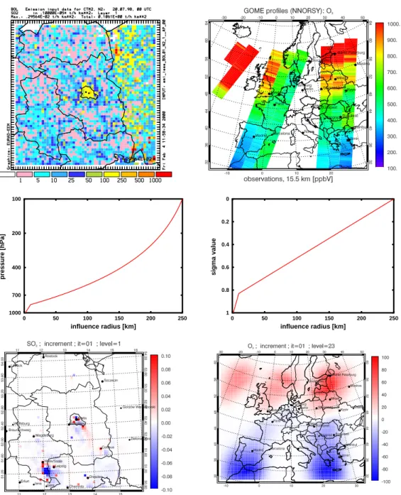
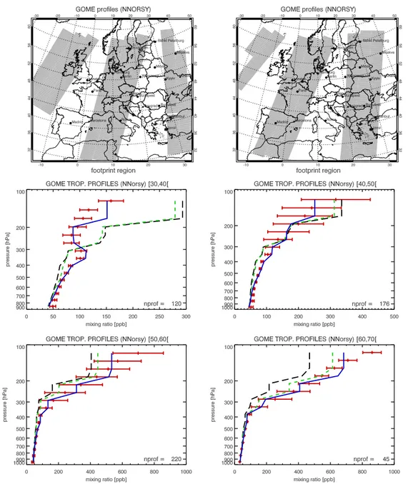
4.1 Parametrisation of horizontal influence radii and their impact on the analysis result. . . 49 4.2 Background emission factors error correlation matrix. . . 52 4.3 Impact of averaging high resolving air-borne measurements. 54 5.1 BERLIOZ: Nested model grid sequence. . . 60 5.2 BERLIOZ CG: Footprints of NNORSY GOME ozone profile

retrievals. . . 63 5.3 BERLIOZ CG: Assimilation results for GOME NO2 tropo-

spheric columns. . . 64 5.4 BERLIOZ CG: Normalised cost function values for ground

based observations with respect to assimilated species and optimisation mode. . . 66 5.5 BERLIOZ CG: Observations and model realisations in grid

cell (43,39,1). . . 67 5.6 BERLIOZ N1: Observations and model realisations in grid

cells (40,40,1) and (40,41,1). . . 69 5.7 BERLIOZ N2: Observations and model realisation for nitro-

gen oxides at selected stations. . . 70 5.8 BERLIOZ N2: Observations and model realisation for hydro-

gen peroxide, sulphur dioxide and formaldehyde at selected stations. . . 71 5.9 BERLIOZ N2: Optimised emission factors. . . 72 5.10 BERLIOZ N2: Surface ozone mixing ratios on July 20. . . . 73 5.11 VERTIKO: Nested model grid sequence. . . 75 5.12 VERTIKO CG: Partial costs by assimilated GOME O3profile

retrievals. . . 77 5.13 VERTIKO CG: Comparison of NO2 column retrievals from

GOME and SCIAMACHY with model equivalents. . . 78 5.14 VERTIKO CG: Temporal evolution of the cost function for

ground based observations. . . 82 5.15 VERTIKO N1: Temporal evolution of cost function for ground

based observations. . . 83 5.16 VERTIKO: Hourly averaged bias and rms. . . 86 5.17 VERTIKO N2: Bias and rms for NH3 campaign data from

June 15 to 19, 2003. . . 93

(9)

List of Figures ix 5.18 VERTIKO N2: Optimised NH3 emission factors for June 18,

2003. . . 94 5.19 Satellite image of Europe and the North-Atlantic on Novem-

ber 14 and 15, 2001. . . 96 5.20 CONTRACE: Model grid sequence. . . 97 5.21 CONTRACE CG: Partial costs by GOME O3 profile retrievals. 98 5.22 CONTRACE CG: O3 profile retrievals by NNORSY from

GOME observations on November 13, 2001. . . 99 5.23 CONTRACE CG: CO mixing ratios during November 14 and

15, 2001. . . 101 5.24 CONTRACE CG: NO mixing ratios on November 14 and 15,

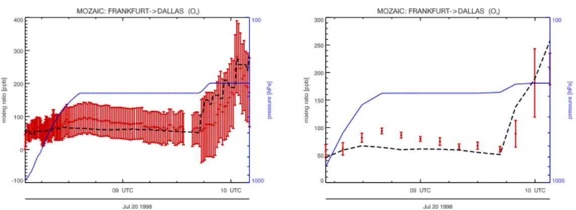
2001. . . 102 5.25 CONTRACE N1: Observational campaign data and MOZAIC

data for O3 and CO on November 14, 2001. . . 103 5.26 CONTRACE N1: Observational campaign data and MOZAIC

data for NO, NO_y and H₂O₂ on November 14, 2001. . . 104 5.27 CONTRACE N1: Partial costs by the campaign data. . . 105 5.28 SPURT: Flight paths of the IOP2 campaign data and avail-

able MOZAIC data. . . 108 5.29 SPURT: Averaged observations and model simulation results

for January 18, 2002. . . 109 5.30 SPURT: Averaged observations and model simulation results

for January 19, 2002. . . 110 5.31 SPURT: Averaged MOZAIC observations and model simula-

tion results. . . 111 5.32 SPURT: Impact of campaign data on model equivalents for

GOME O3 profile retrievals. . . 112

(10)

(11)

List of Tables

2.1 Definition of model variable notation. . . 9 4.1 Standard deviations of the transformed emission factors. . . 50 5.1 BERLIOZ: Simulation setup. . . 59 5.2 VERTIKO: Simulation setup. . . 74 5.3 VERTIKO: Bias and rms for satellite column retrievals. . . . 77 5.4 VERTIKO: Bias and rms statistics for ground based stations. 85 5.5 CONTRACE: Simulation setup. . . 95 5.6 CONTRACE: Bias and rms statistics. . . 98 5.7 SPURT: Simulation setup. . . 107 5.8 SPURT: Bias and rms error for GOME O3 satellite profiles. 113 A.1 Vertical grid structure for the 23 layer design. . . 119 A.2 Vertical grid structure for the 26 layer design. . . 120 B.1 Minimum estimates for the absolute background errors. . . . 123 B.2 Absolute and relative measurement errors for ground based

stations. . . 124 B.3 Absolute representativeness error estimates at surface level. . 125 B.4 Representativeness lengths for ground based observations. . . 125

(12)

(13)

List of Acronyms

4d-var Four-Dimensional Variational

AK Averaging Kernel

BERLIOZ Berliner Ozon Experiment BLUE Best Linear Unbiased Estimate

CONTRACE Convective Transport of Trace Gases into the Upper Troposphere over Europe: Budget and Impact on Chemistry

CTM Chemistry Transport Model

DLR Deutsches Zentrum f¨ur Luft- und Raumfahrt DOAS Differential Optical Absorption Spectroscopy ECMWF European Centre for Medium-Range Weather Fore-

casts

EEA European Environment Agency

EEM EURAD Emission Model

EMEP Co-operative programme for monitoring and evalu- ation of the long-range transmissions of air pollu- tants in Europe

EURAD European Air Pollution and Dispersion [model]

GMES Global and regional Earth-system Monitoring using Satellite and in-situ data

GOME Global Ozone Mapping Experiment IOP Intensive Observational Period

(14)

KF Kalman Filter

KNMI Koninklijk Nederlands Meteorologisch Instituut

KPP Kinetic PreProcessor

L-BFGS Limited-Memory Broyden Fletcher Goldfarb Shanno MM5 Fifth-Generation NCAR / Penn State Mesoscale

Model

MOZAIC Measurements of Ozone and Water Vapour by in- service Airbus Aircraft

NCAR National Center for Atmospheric Research NNORSY Neural Network Ozone Retrieval System

PROMOTE Protocol Monitoring for the GMES Service Element RACM Regional Atmospheric Chemistry Mechanism RADM Regional Acid Deposition Model

SCIAMACHY Scanning Imaging Absorption Spectrometer for At- mospheric Chartography

SPURT Trace Gas Transport in the Tropopause Region UTC Coordinated Universal Time

UT/LS Upper Troposphere/Lower Stratosphere

VERTIKO Vertical Transport of Energy and Trace Gases at Anchor Stations and Their Spatial/Temporal Ex- trapolation under Complex Natural Conditions VOC Volatile Organic Compounds

(15)

CHAPTER 1 Introduction

Studying atmospheric processes has always been motivated by the desire to predict future system states. Bjerknes[1911] formulated such a forecast as a deterministic initial value problem: ”The solution of a system of differential equations with concrete initial values can lead to a weather forecast. But as a matter of fact, a good prediction always needs an exact guess of the atmosphere’s actual state.” Until the 70ies of the last century, observations scattered in time have been used to draw synoptical maps. Not before the advent of numerical models and their computational efficiency, weather forecasts relied on subjective analyses of the current physical state of the atmosphere. When suitable error characterisations or probability density functions of the available information have been specified, this allows for an objective analysis in terms of the most probable system state. The technique of statistical interpolation (Eliassen [1954], Gandin [1963]) was more and more used in all fields of geophysical interest. It is,e. g., known as Gauss-Markovalgorithm in oceanography and asKrigingmethod in applied geophysics. Subsequently, objective analysis by data assimilation gained acceptance in meteorology (Daley [1991]).

The observational basis in meteorology as well as in atmospheric chemistry changed substantially within the last decades. In addition to enhanced ground based observational networks with a denser set of measurement stations, satellite based remote sensing data is now available at high resolution levels and with remarkable global coverage.

(16)

Hence, new observation techniques favoured the use of spatio-temporal techniques as the four-dimensional variational (4d-var) algorithm (e. g.,Courtier [1997]) and the Kalman Filter (Kalman[1960],Kalman and Bucy[1962]), in order to fully use the information contained in the heterogeneous observation types. In contrast to sequentially employed spatial algorithms, which do not use physical or chemical constraints to join the scattered information, spatio-temporal algorithms allow the fusion of both heterogeneous observations and the physical and chemical laws coded in numerical models. These algorithms are used to retrieve analyses, that lead to consistent system evo- lutions and that are available on regular grids. In the field of meteorology, the 4d-var method entered operational weather forecasting in the nineties.

The most prominent example is the first operational 4d-var implementation at the ECMWF in 1997 (Rabier et al. [2000]), while all meteorological cen- tres thereafter experienced substantial benefits from going to 4d-var (Rabier [2005]).

During the last decade much progress has been attained in developing com- prehensive chemistry transport models for both the stratosphere and the troposphere. In concert with rapidly increasing computer power and lab- oratory results on new chemical reaction paths, spatially highly resolved model simulations with sophisticated chemistry kernels and promising forecast behaviour over longer periods have become available. In addition to user-oriented air quality forecast services¹, long-term model simulations are used for episodic assessments of suitable political regulations to enhance the air quality in Europe (Memmesheimer et al. [1996], Memmesheimer et al.

[2004b])².

Moreover, spatio-temporal data assimilation algorithms have been introduced in the field of atmospheric chemistry, exhibiting a development comparable to the development in meteorology, with 20 years delay, however.

The usefulness of the variational approach for atmospheric chemistry has been shown by Fisher and Lary [1995] with box model simulations for the stratosphere. The spatio-temporal extension with the 4d-var technique for the full tropospheric chemistry kernel RADM2 has been applied by Elbern et al. [1997]. Elbern and Schmidt [1999] extended the regional EURAD model to the first available complete adjoint chemistry transport model for the troposphere, including parallelisation, pre-conditioning and off-diagonal covariance modelling. Further, the real world applicability for an ozone case study has been shown inElbern and Schmidt [2001].

The application of advanced data assimilation techniques using complex

1Visit, e. g.,www.gse-promote.org/services/airquality.htmlfor a short overview.

2For a list of German clean air plans surf towww.umweltbundesamt.de/luft/index.htm.

(17)

3 chemistry transport models has only become feasible since the last decade, due to several reasons: Firstly, realistic chemical systems include at least ten times more control parameters (chemical species, see Stockwell et al. [1990]

or Sander et al. [2005]) than those used in meteorology or oceanography.

This influences the complexity of statistics concerning covariance models as well as the demands in computer power. Secondly, there is a huge imbalance between available measurements and model parameters. The number of observations is usually far below the number of parameters in a chemistry transport model, such that the system is grossly underdetermined (it may as well be locally overdetermined). Additionally, there is not necessarily a straight forward model equivalent to each kind of observation due to the often lumped formulation of the chemical reaction schemes or due to some methods of measuring, where classes of species are observed as single quantity.

Another reason is the more complicated way in which the forecast skill of the atmospheric chemistry is influenced by initial values. At least in the troposphere, there might be several other processes which have a signifi- cant impact on the temporal evolution of the system like emission rates and deposition velocities. Especially emission rates have a strong influence on the trace gas concentrations, at most in the vicinity of the sources.

Moreover, hourly emission rates are calculated on the basis of annually emitted amounts, given on a presumably different inventory grid, and thus are subject to huge uncertainties. However, due to a possibly strong ex- change between the atmospheric boundary layer and the free troposphere, the emissions can strongly influence large model areas by long-range transport. Hence, a number of source and sink estimation assessments have been conducted: Kaminski et al. [1999] estimated CO2 fluxes using a 4d-var implementation in the TM2 model and global observations. The first 4d-var implementation for a complete set of emitted species was introduced byEl- bern et al. [2000], who additionally showed the applicability with identical twin experiments for the EURAD model. Qu´elo et al.[2005] used a one year comparison of observations and simulations with the POLAIR3D model to retrieve NOx emission time distribution, which exhibits to be robust and which significantly improved ozone forecast skills. The combination of emission rate and chemical state optimisation of precursor trace gases with 4d-var by observations of product species and a systematic assessment of improved forecast quality by observations withheld from the assimilation procedure is shown inElbern et al.[2006] for an ozone episode. Hence, best estimates also for surface fluxes are indispensable for good predictions of the chemical composition.

(18)

However, despite the attained complexity and the sophistication level of the 4d-var data assimilation algorithm, the following problems still prevent the achievement of high quality tropospheric model simulations:

(i) Fine model resolutions are needed in order to predict primary emitted species like nitrogen oxides, which exhibit strong spatial gradients. Other- wise, for example, the ozone chemistry simulations may reside in a wrong chemical regime. Moreover, enhanced model resolution will significantly reduce biases in the representativeness of assimilated observations for the grid cells. The favourable option to increase the model resolution are nested sub-domains, which, as a by-product, lead to optimised boundary values in terms of analysed model states from the respective mother domain.

To this end, an adjoint nesting approach has been developed in this work, allowing to telescope from regional scale down to local scale. The benefit of this facility for forecast skills and the analysis quality is addressed in boundary layer campaign simulations.

(ii) One of the most crucial aspects of spatio-temporal data assimilation is the treatment of background error covariances. Both the estimated variances of the background fields as well as their correlations manifest the quality of an analysis, at most in data void regions. By reason of the size of one model state vector, the background error covariance matrix for com- prehensive chemistry transport models cannot be treated numerically in a straight forward way. One option is to provide it as an operator instead of its matrix representation. Further, due to surface textures and corre- sponding correlation features in the background state, an inhomogeneous and anisotropic design is eligible.

To this end, a diffusion operator is employed in this work to construct the correlations in the initial value background error covariance matrix. This enables to flexibly model covariances in the background fields and can be easily extended to represent anisotropic and inhomogeneous correlations.

Additionally, for the optimisation of emission rates, a background error covariance matrix has been coded from scratch, allowing to model reasonable correlations between different emitted trace gases and to reduce the degrees of freedom in the analysis procedure. Both covariance matrices now admit to simultaneously optimise the initial model state and emission rates in a balanced and suitably preconditioned way.

(iii) To allow for the use of all available information during a data assimilation procedure in the best possible manner, a suitable observation operator needed to be constructed. This facilitates the confrontation of a model simulation with remote sensing data like tropospheric column and profile retrievals from satellite observations, lidar and tethered balloon soundings,

(19)

5 as well as air-borne and ground based in-situ data. The use of air-borne and satellite measurements is discussed for a data assimilation suite of two air-borne campaigns, focussing on the free and upper troposphere.

Hence, the main intention of this work is to demonstrate the feasibility of sophisticated spatio-temporal data assimilation for the modelling of tropospheric chemistry from mesoscale down to local scale and its favourable impact on the forecast skill. The chosen algorithm is the 4d-var method, which is introduced and shortly compared to the Kalman Filter in Chap- ter 2. The extensions and improvements of the EURAD 4d-var data assimilation system developed in this thesis — namely the adjoint nesting technique, the technique of a balanced joint estimation of initial chemical state and emission rates, an improved chemistry solver with an updated mechanism, and the observation operator — will be shown in Chapter 3 in the framework of a concise system description. The modelling of the variances and covariance matrices involved in the assimilation procedure can be found in Chapter 4. The complete model system is then applied to four campaign data sets, in slightly different configuration with varying subject matter. The results of which are detailed in Chapter 5. Finally, Chapter 6 summarises and discusses the results of this thesis.

(20)

(21)

CHAPTER 2 Data Assimilation

The main objective of data assimilation is to provide an as accurate as possible and consistent image of a system’s state at a given time (the optimal guess) by taking into account all available information about the system.

This information may consist of

1. observations providing samples of the system’s current state,

2. the intrinsic laws of the system’s evolution in space and time, coded in a numerical prognostic model, and

3. a previous estimate of the true state (encompassing all information gathered in the past), usually referred to as thebackground knowledge.

Combining all these types of information, the observed knowledge may propagate to all state variables of the model, while the model provides for the constraints on the propagation within the system. Hence, the innovation can accumulate in time (Bouttier and Courtier [1999]), being the core principle of all model based data assimilation techniques. It is however affected by errors of often poorly known quantities (e. g., biases, discretisation errors). Observations usually vary in nature and accuracy and are strongly irregular distributed in space and time. Concerning atmospheric chemistry, only a few system’s instances are observed (i. e., chemical species) and often there is a lack of validated error statistics. So none of this available information is exactly true. We cannot ”trust” completely neither the model,

(22)

nor the observations, nor the a-priori information (which may consist of climatological statistics, the result of a previous analysis, a model forecast or combinations of those), since they are affected by uncertainties. This leads to the formal requirement to take into account the data errors (their probability distribution functions) such that the resulting analysis error is minimal. In some suitable sense this will allow us to write the analysis problem as an optimisation problem. The following section will present this in the framework of least-squares estimation.

For a detailed classifications of data assimilation techniques and the history of data assimilation in meteorology see Lorenc [1986], Ghil [1989], Daley [1991] andTalagrand [1997].

2.1 Objective Analysis using Least-Squares Estimation

To derive the most common data assimilation techniques we need first to assume some properties of the error variances of the input parameters. The error estimation and the generalisation to covariances will evolve throughout this work, namely when introducing the data assimilation algorithms in the next sections, in Chapter 4 and Appendix B. The notation given in Table 2.1 will be used, following as close as possible the suggestions given inIde et al.

[1997].

2.1.1 Definition of errors

The background errors or forecast errors

ε^b =x^b−x^t (2.1)

are the only terms that separate the background knowledge from the true state (Bouttier and Courtier [1999]). They are the estimation errors of the background state, which is the best model based guess of the system’s current state. The errors represent both the uncertainties in the up-to- now knowledge and the forecast errors, if a model integration was used to produce the background model state.

The observation errors

ε^o = (y^t−H(x^t))

| {z }

ε^r

+ (y−y^t)

| {z }

ε^m

=y−H(x^t)

(2.2)

(23)

2.1 Objective Analysis using Least-Squares Estimation 9 include the errors due to the statistical performances of the measuring in- struments (ε^m) and an estimate of representativeness error (ε^r). H is the observation operator or forward interpolation operator that generates the model equivalentsto the observations in the case that both the observations and the model state vector were true and that there are no forecast errors.

In practise H is a collection of interpolation operators from the model discretisation to the observational points and conversions from model variables to the observed parameters. Some remarks on the properties of H as implemented in the EURAD 4d-var system are given in Section 3.6.

The representativeness error reflects the degree to which an observation is able to represent the optimal model equivalent H(x^t), basing on volume- average model state values. Representativeness errors are usually taken to be unbiased, and their magnitudes may depend on the volume size, the sensor’s time average, the volume size which one wants the observation to represent, and the chemical state of the atmosphere. This error has to be included in the observational error (Daley [1991]).

Table 2.1: Definition of model variable notation. The number of observations is denoted byp, while a vector of an initial model state and the emission factors is of sizen and m, respectively.

Parameter Definition Dimension

x^t true model state n

x^b background model state n

x^a analysis state n

y observations p

y^t true observational state p

H observation operator —

H linearised observation operator p×n B background error covariance matrix

(initial values)

n×n K background error covariance matrix

(emission factors)

m×m O measurement error covariance matrix p×p F representativeness error covariance

matrix

p×p R=O+F observation error covariance matrix p×p A analysis error covariance matrix n×n

(24)

The terms [y−H(x)] are calleddeparturesor theinnovation vectorand are the key to data analysis based on the discrepancies between observations and model states (Parrish and Derber[1992]).

We assume those errors to be unbiased,

hε^bi= 0 and hε^oi= 0, (2.3) where hi is the expectation operator. Additionally, we consider the observational and the background errors to be mutually uncorrelated, i. e.

hε^bε^oi= 0. (2.4)

The analysis errors

ε^a =x^a−x^t (2.5)

is what we want to find, such that the analysis is optimal in the sense that it is as close as possible to the true model state x^t.

2.1.2 Minimum variance and maximum likelihood

What we are looking for is an optimal estimation for the analysisx^a. Con- sider the problem of estimating a scalar parameterxwith x^t being the true value, having p measurements yi,1 ≤ i ≤ p with measurement errors εi

(seeDaley [1991]). The expected error variances are denoted σ_i² =hε²_iiand suppose the errors are unbiased and uncorrelated (as described above). The estimate x^e should be a linear composition of the observations:

x^e =X

i

ciyi,

withci ≥0 fori= 1, . . . , pbeing the weights to be specified. ε^edenotes the error of the estimate. The bias then reads

hε^ei=hx^ei − hx^ti=X

i

cihεii − hx^ti

"

1−X

i

ci

# .

(25)

2.1 Objective Analysis using Least-Squares Estimation 11 We attain an unbiased linear estimate hε^ei = 0 if P

ici = 1. For the expected error variance we yield

h(ε^e)²i=h(x^e−x^t)²i

=

* X

i

ciyi−X

i

cix^t

!2+

=

* X

i

ciεi

!2+

=X

i

c²_iσ_i²

(2.6)

The minimum variance estimate is now defined to be the estimate x^a that minimises (2.6). This may be solved by the method of Lagrange’s undeter- mined multipliers. The solution is characterised as follows: The minimum variance estimate or the optimal linear unbiased estimate (also called best linear unbiased estimate or BLUE) is given by

x^a = P

iσ_i⁻²yi

P

iσ_i⁻² . (2.7)

The minimum error variance reads h(ε^a)²i=X

i

c²_iσ_i² = 1 P

iσ⁻²_i

or 1

(σ^a)² =X

i

1 σ²_i.

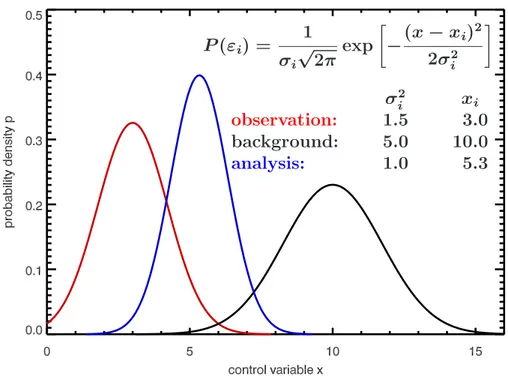
Each additional observation thus reduces the expected error varianceh(ε^a)²i of the minimum variance estimate. Therefore the expected error variance is always smaller than the least expected error variance of y (see Fig. 2.1 for an example of p= 2 and Gaussian distributed errors).

For Gaussian distributed error probabilities P(εi) = 1

σ_i√

2πexp

− ε²_i 2σ_i²

the joint error probability of allp observations is given by P(ε1)P(ε2)· · ·P(εp) =Y

i

1 σi

√2π exp

− ε²_i 2σ_i²

=

"

Y

i

1 σ_i√

2π

# exp

"

−X

i

(yi−x^t)² 2σ_i²

# .

(2.8)

(26)

P(εi) = 1 σ_i√

2π exp

−

(x−x_i)² 2σ_i²

σ²_i xi

observation: 1.5 3.0 background: 5.0 10.0

analysis: 1.0 5.3

Figure 2.1: Example for a minimum variance/maximum likelihood estimate for p = 2 (the second ”observation” is for future reference called background) and Gaussian probability distribution functions. The analysis distribution is the best linear unbiased estimateBLUE, which has a higher probability of the expectation value and a smaller variance than both observations (a sharper pdf ).

The most probable valuex^a is that one which maximises (2.8). This occurs when the argument to the exponential function reaches a minimum. The maximum likelihood estimatemust minimise

J = 1 2

X

i

σ_u⁻²(x^a −yi)². (2.9) Differentiating with respect tox^a and setting the result to zero leads to

x^a = P

iσ_i⁻²yi

P

iσ_i⁻² ,

which is the same as (2.7). When error distribution is Gaussian, minimum variance and maximum likelihood estimates thus lead to the same optimal linear unbiased estimate (or BLUE).

The following sections discussing advanced data assimilation techniques will generalise (2.7) and (2.9) under different constraints.

(27)

2.1 Objective Analysis using Least-Squares Estimation 13

2.1.3 Conditional probabilities

The analysis problem can be described in terms of conditional orBayesian probabilities (Lorenc[1986]). These probabilities are based on the Theorem of Bayes defining the joint pdf of two events x and y

P(x|y)P(y) =P(y|x)P(x), (2.10) whereP(x) denotes the probability of an event xto be true and P(x|y) the probability of the event x under the condition of event y to be true. This theorem is useful for cases in which there is an eventy that can be observed while there is an event x that has to be determined.

Let us consider a set of observations Yj = {y0, y1, . . . , yj} gathered in a time window [0, tj], j = 0, . . . , N and a model state x to be determined, conditional to the informationYj. We then yield (Cohn [1997])

P(x|Yj) =P(x|yj, Yj−1) = P(x, yj, Yj−1) P(yj, Yj−1)

= P(y_j|x, Y_j−1)P(x, Y_j−1) P(yj, Yj−1)

= P(y_j|x, Y_j−1)P(x|Y_j−1)P(Y_j−1) P(yj|Yj−1)P(Yj−1)

= P(yj|x, Yj−1)P(x|Yj−1) P(yj|Yj−1) ,

(2.11)

which is only another version of Bayes’ rule. This very general result can be used to derive the data assimilation techniques presented below under different constraints and assumptions, because it delivers a method to derive P(x|Yj) fromP(x|Yj−1);i. e., the analysis update using a newly introduced information yj and the background information pdf P(x|Yj−1). It is both the basis of conditional mean estimation, which is identical to the minimum variance estimator, as well as of conditional mode estimation, resulting in the maximum likelihood estimator. In the former case, the result forxwill be the expectation value ofP(x|Yj) (under the assumption of its existence), where in the latter case the numerator of (2.11) is evaluated for a maximum, resulting in the most probable value of x. This will be done in Section 2.3 to derive the objective function describing the 4d-var method.

This fundamental probabilistic formalism of the analysis problem may be generalised to arbitrary probability distribution functions leading to the possibility to account for control variables which have strongly non-Gaussian error pdfs, like log-normal distributions. In some recent works this is ac- counted for (e. g., Fletcher and Zupanski[2006]).

(28)

2.2 Optimal Interpolation and Kalman Fil- tering

This section very briefly introduces two important data assimilation methods that attempt to minimise analysis errors by minimum variance (or conditional mean estimator) algorithms.

Optimal interpolation — often referred to as statistical interpolation — is still widely used in atmospheric data assimilation. The method reads as follows:

With the notation defined in Section 2.1 we write the analysis increment (x^a−x^b) as a linear combination of the observation departures (or innova- tions),

x^a =x^b+K(y−H(x^b)), (2.12) where the matrix K contains the weights to be determined. Here the observations may be displaced to the model grid points, so that we need to calculate the model equivalent of the observations by applying the observation operator H to the model state. For convenience we consider the observation errors and the background errors to be unbiased and mutually uncorrelated (Eqs. (2.3)-(2.4)).

Under the condition, that the optimal weightsKare encountered, when the analysis error is minimal, the result can be shown to be (e. g.,Daley [1991])

K=BH^T

R+HBH^T−1

, (2.13)

where K is referred to as the gain matrix and H is a linear observation operator, linearised in the vicinity of the background model statex^b, such that

H(x)−H(x^b) =H(x−x^b) +O

(x−x^b)²

is satisfied (Bouttier and Courtier [1999]). The algorithm (2.12) is only optimal if the covariance matricesBandRand the forward operatorHare correct.

Until the late nineties Optimal Interpolation was the most common used data assimilation technique — at least in operational weather forecast and chemistry transport models (Talagrand [1997]). It was well suited for the demands of operational forecasting because the implementation of (2.12) only needed the inversion of (R+HBH^T). The algorithm can be performed in asequentialmode, which means that the analysis procedure is performed each time a new observation is available. The result of the analysis step is taken as initial state for a model forecast until the next analysis time. This

(29)

2.2 Optimal Interpolation and Kalman Filtering 15

x

time observation

analysis run control run

Figure 2.2: Principle of sequential data assimilation algorithms, shown for one single model parameter. At each analysis instance the model state is updated by the newly introduced observations. If there are only a few instances of the system measured, the successive model integration forward in time relaxes the usually distorted model state towards the control run, due to the chemically coupled evolution of the whole system.

scheme is depicted in Fig. 2.2 for a single model variable. This primitive sketch already shows some of the properties of statistical interpolation: At each analysis instance (here the observational times) the model state is corrected to the BLUE analysis state given by the observation and the a-priori model state. This usually leads to an analysis model state which is (chemically) distorted and the correction often vanishes after a short successive forecast period — i. e., the model trajectory relaxes towards the background state.

Let us now introduce a prognostic model description by dx

dt =M(x) +η (2.14)

where M is a linear model describing the time dependence of the model state, being itself independent from model state x and having errors η

(30)

with covariances Q. Having an analysis state x^a_j−1 at time t = tj−1 for j = 1, . . . , N, we can write the forecast step tj−1 →tj as

x^f_j =Mjx^a_j−1+η, (2.15) where Mj denotes the model operator propagating the model state from x_j−1 to x_j. With the same assumptions as in (2.12) we can derive the related forecast error covariance matrixP^f_j to (see Daley [1991])

P^f_j =MjP^a_j−1M^T_j +Qj−1. (2.16) The analysed variables evolve from the forecast by the following formulas

x^a_j = x^f_j+Kjd_j (2.17)

P^a_j = (I−KjHj)P^f_j, (2.18) whered_j = (y−Hx^f_j) denote the innovation vector and

Kj =P^f_jH^T_j(HjP^f_jH^T_j +Rj)⁻¹ (2.19) is the Kalman gain matrix. Eqs. (2.15-2.18) define the discrete Kalman Filter (Kalman [1960], Kalman and Bucy [1962], Jazwinski [1970]), which is the minimum variance solution to the analysis problem under the condition that both the model and the observation operator are linear. This algorithm exploits all available information and successively updates the analysis error covariances (and thus delivers the background error covariances for the next step). This part of the Kalman Filter is the by far most demanding procedure, because (2.16) involves large matrix multiplications.

Therefore, the application of the Kalman Filter in concert with large numerical models is still impossible (Loon and Heemink [1997], Bouttier and Courtier [1999], Constantinescu et al. [2006]). It is mostly applied in sub- optimal versions, e. g. the Ensemble Kalman Filter (EnKF, Houtekamer et al.[2005]) or the Reduced Rank Square Root Kalman Filter (RRSQRT, Heemink et al.[2001]). For an elementary comparison of the Kalman Filter and the 4d-var data assimilation technique see Section 2.4.

2.3 4D-Var Data Assimilation

Using variational data assimilation techniques, the analysis problem is formulated as a minimisation problem of the variational calculus (see, e. g., Courant and Hilbert [1953]). A objective or cost function is defined, measuring the distance between a model simulation and the observations (see

(31)

2.3 4D-Var Data Assimilation 17 Eq. (2.9)). To derive the cost function from (2.11), we need to define both the properties of the mapping between the model phase space and the observational phase space (i. e., the forward model H) and of the prognostic model M itself. We want to use the model as a strong constraint to the optimisation problem. Therefore the model is regarded to be perfect and the errorηvanishes in (2.14). Further, we assume that there are no stochas- tic processes influencing the model development in time, which makes the model deterministic. This leads to

∀j, x^t_j =Mjx^t_j−1, (2.20) where x^t_j is the true model state at time t =tj and Mj a predefined non- linear model operator performing the integration from timetj−1totj. Hence we can describe the model evolution from the initial state x₀ to the state x_j by recurrence,

x_j =M_jM_j−1 . . . M₂M₁x₀. (2.21) Under the assumption, that a current observationy_j is independent from the set of previous observations Yj−1 and with the properties of the prognostic model given above, we can rewrite (2.11) as

and P(x|Yj) is the posterior pdf.

In Section 3.4 there will be a brief introduction to the kind of model parameter that is amenable to variational data assimilation under a certain observational basis. Moreover, the formulation of the cost function is de- vised for the combination of initial values and emission rates as control parameters. For the sake of convenience we will now assume, that the initial state of the model integrationx₀ is the only set of parameters which is subject to the minimisation procedure — i. e., the set of parameters to be analysed. The background knowledge is denotedx^b and yis a set of observations, being distributed in space and time and vector valued for each time instance. Considering the first term on the right side of (2.22) constituting the background model state based on the information available before the time instance for which the new informationyj is introduced, and assuming that Gaussian distribution functions sufficiently describe the properties of

(32)

both the background errors and the observation errors, we yield P(x₀|Y)∝exp

−1 2

x₀−x^bT

B⁻¹

x₀−x^b

× exp

(

−1 2

XN

j=0

y_j −Gj(x0)T

R⁻¹

y_j−Gj(x0)) ,

(2.23)

where Gj is the combination of forward operator Hj and model operators M, reading

Gj :={HjMjMj−1 · · · M1} and M0 =I

generating the model equivalent of the observations at timetj, when applied to the initial state. The covariance matrix of the observation errors is given by R, andN denotes the time index t_N —i. e., the end of the assimilation window.

The principle of 4d-var is defined by finding the maximum likelihood estimation of x₀ by iteratively maximise its conditional probability (2.23), which is identical to the problem of minimising the scalar valuedobjective functionor cost function J,

J(x₀) = −log [P(x₀|Y)]

=Jiv+Jobs

=1 2

x₀−x^bT

B⁻¹

x₀−x^b + 1

2 XN

j=0

y_j −Gj(x₀)T

R⁻¹

y_j−Gj(x₀) .

(2.24)

The minimisation is usually achieved by calculating the gradient of the cost function with respect to the control parameters x₀, given to a standard gradient descent minimisation algorithm performing successive iterations.

This gradient can be obtained numerically in different ways. The most effi- cient way for high dimensional problems like in chemical data assimilation uses principles of the theory of adjoint equations and can be described as follows:

The application of the prognostic model to small variations δx0 and lin- earising the result leads to

δxj =MjMj−1 · · · M1δx0, (2.25) where the Jacobians with respect to the state variable

Mj := ∂Mj

∂xj

x_j

(2.26)

(33)

2.3 4D-Var Data Assimilation 19 are linearised model operators, referred to as thetangent linearmodel. Un- der the assumption of both a linear model and a linear forward operator — G_j is linear in x_j, the cost function (2.24) is a quadratic form and has a unique minimum. Hence, the minimisation will lead to an optimal guess of the initial values. On the validity of thetangent linear approximation(i. e., the linearisation of both the model and observation operator still leads to a nearly optimal analysis) the reader may refer to Courtier et al. [1994], Talagrand [1997],Cohn [1997] and Bouttier and Courtier [1999].

We want to derive a formula for the gradient of the cost function with respect to the initial values. Therefore, using the canonical scalar product

<a, b >= P

ia^T_i bi (note the difference to h·i denoting the expectation value), we first describe small variations of the scalar valued function J(x) as a result of small variationsδx

δJ ≈<∇^xJ , δx> .

Hence, the following holds for the observational termJobs in the cost function (2.24):

δJ_obs = XN

j=0

<∇^xjJ_obs, δx_j>

Introducing the tangent linear model equation (2.25), small variations in the cost function are obtained as a result of small variations in initial conditions:

δJobs = XN

j=0

<∇^xjJobs, MjMj−1 · · ·M1δx0> . (2.27) Using <a, Qb>=<Q^Ta, b>, where the superscript T denotes transpo- sition, we can rewrite (2.27) to

δJobs = XN

j=0

<M^T₁ M^T₂ · · · M^T_j ∇^xjJobs, δx0> ,

where M^T_j are the adjoint operators to the tangent linear model (2.25).

Thus the gradient of the cost function with respect to the initial conditions is given by

∇^x⁰J =∇^x⁰(Jiv +Jobs)

=B⁻¹

x₀−x^b +

XN

j=0

M˜^T_jH^T_jR⁻¹

y_j −Gj(x0)

, (2.28)

(34)

whereJiv is the cost function with respect to the updated initial values. H^T is the adjoint operator of the linearised forward operator and

M˜^T_j :=

Y0

i=j

M^T_i (2.29)

is the adjoint model performing the integration fromt=tj tot=t0. Consequently, the gradient of the cost function with respect to the initial values can be obtained by integrating the direct model forward in time fol- lowed by an adjoint model integration backward in time. At the end of the forward integration, the adjoint model state, here denoted by x^∗, is initialised with x^∗ = 0. This adjoint model state is integrated backward in time using the adjoint model operators. At each time instanceti, for which a new set of observationsy_j is available, the state of the adjoint integration is updated by the observational forcing term y_j −Gj(x0) = y_j −Hj(xj).

At the end of the integration, the gradient of the cost function with respect to the initial values is given by the final state of the adjoint model run. The main advantage of this algorithm is that it allows to calculate a complete and accurate gradient of the cost function with one direct (forward) integration and one successive adjoint (backward) integration of the model, which is numerically much cheaper than a perturbation method. The disadvan- tages are at hand: First, the adjoint model operators have to be coded and, second, the forward model states have to be completely available prior to the adjoint integration.

The former problem means, that a new model has to be developed as complex as the forward model. This can be achieved in various ways: One possibility is to adjoin the system of model equations with its own formulation, discretisation and linearisation (if needed). Another possibility is to derive the tangent linear of a piece of code and to adjoin line by line (Talagrand [1991], Schmidt [1996], Giering and Kaminski [1998]), which preserves the forward formulation and discretisation. Nowadays there areadjointcompil- ers that help creating adjoint pieces of code, for example TAMC (Giering [1999]) andOδyss´ee (Faure and Papegay [1998]).

The second problem is due to the fact that the forward model trajectory explicitly appears in the observational forcing terms and that it additionally needs to be available in order to get the right adjoint operator of the tangent linear solution (2.25), in the case of a non-linear forward model M and/or observation operatorH. This leads to storage demands, which are still unfeasible using a model with a phase space size of order 10⁶, which is the case for the EURAD chemistry transport model (see, e. g., Schmidt [1999]).

(35)

2.3 4D-Var Data Assimilation 21

t0 tN

x^a x^b

time

assimilation window

control run x

observations

analysis run

Figure 2.3: Principle of 4d-var data assimilation algorithm, here for one single model parameter. Because 4d-var fits a model trajectory to a set of observations within the predefined assimilation window, it is a smoother algorithm. The result is aBLUE for each time step.

The solution to these problems as implemented in the current EURAD 4d- var data assimilation system will be shown in Section 3.1.

Minimising the cost function (2.24) under the nonlinear constraint (2.20) — provided errors are Gaussian — will produce a BLUE of the system under consideration at any timetj ∈[t0, tN], if the tangent linear assumption holds in the neighbourhood of x^b and the error statistics are unbiased and correct (Lorenc[1986]). Due to the fact that it propagates information forward and backward in time, 4d-var is regarded asmoother, fitting a model simulation to a set of observations distributed in a predefined time window (see Fig. 2.3). This is in contrast to the principle of filtering, propagating information forward in time only (cf.Section 2.2). Many applications of 4d- var to real data experiments in meteorology, oceanography and atmospheric chemistry exhibit the capability of minimising efficiently the penalty function even under non-linear model constraints (see, e. g., Talagrand [1997]

and references therein). Due to its formulation, 4d-var is able to produce physically and chemically consistent model simulations within the whole assimilation window and therefore to analyse even constituents which are not observed or to propagate information to data void regions.

(36)

2.4 4D-Var vs. KF

The 4d-var method and the Kalman Filter (KF) are spatio-temporal algorithms, which exploit the available information about the system state on the highest sophistication level. Under the assumption of a perfect model, that is that the model errorη in (2.14) vanishes, both methods lead to the same analysis at the end of the 4d-var assimilation window. However, ”the ambitious and elusive goal of data assimilation [...] to provide a dynamically consistent motion picture of the atmosphere and oceans, in three space di- mensions, with known error bars” (Ghil and Malanotte-Rizzoli [1991]), can only be provided by the Kalman Filter without recourse to features of the minimisation solver. It has the certain appeal of integrating the initial background error covariance matrix in time, leading to forecast and analysis error covariance matrices, fulfilling the elusive goal mentioned above.

An estimate of the analysis error covariance matrix by the 4d-var method can be yielded by, for example, singular value decomposition, which is used in a limited memory version by the current model version as minimisation routine (see Section 3.2). However, this method is of about the same complexity as the 4d-var method itself (Elbern[2001]).

Kalman Filtering comes with huge computational demands in the framework of large numerical models. This allows its application in atmospheric chemistry only for models of a strongly reduced complexity. Another method to supersede the unfeasibility is to reduce the complexity of the Kalman Fil- ter itself (see Section 2.2), leading to very promising results in the stratosphere as well as in the troposphere. The advantage of those algorithms is the easy implementation, compared to the need to code the adjoint model version in the framework of 4d-var. While the KF serves for propagated covariance matrices, the analysis by 4d-var is physically and chemically consistent over the whole assimilation window without intermittent breaks at observation times.

Besides real data comparisons of 3d-var and the Ensemble Kalman Filter (EnKF) in the operational meteorological framework (Houtekamer et al.

[2005]), first parallel implementations of EnKF and 4d-var in state-of-the- art chemistry transport models show small predominance of 4d-var during the assimilation window, while comparable results are achieved for both methods in subsequent forecasts (Constantinescu et al. [2006]). Possible future developments will take into account and exploit both methods.

(37)

CHAPTER 3 The EURAD 4D-Var Data Assimilation System

The EURAD (EURopean Air pollution and Dispersion) data assimilation system consists of four main parts, the EURAD model system, the adjoint chemistry transport model (ADCTM), the minimisation procedure L-BFGS¹ including a preconditioning module, and the observational data preprocessor PREP, collecting available observations and providing them in a standardised file.

The EURAD model system is an advanced numerical model system able to simulate the physical and chemical evolution of trace gases in the troposphere and lower stratosphere (Hass [1991], Hass et al. [1995], Petry et al.

[1997]). It consists of the meteorological driver MM5² (Grell et al. [1994]), the EURAD emission model EEM (Memmesheimer et al. [1991]) and the EURAD chemistry transport model (EURAD-CTM). The EURAD-CTM is a mesoscale chemistry transport model involving transport, diffusion, chemical transformation, wet and dry deposition of tropospheric trace gases (Hass [1991], Memmesheimer et al. [1997]). It is used for long term simulations focussing on emission directives and their influence on air quality (Memmesheimer et al. [2000], Memmesheimer et al. [2004]) as well as for operational forecast from hemispheric down to local scale using nesting tech- niqueJakobs et al.[1995] and episodic scenarios focussing on special aspects

1limited memory BroydenFletcherGoldfarbShanno

2developed at the National Center for Atmospheric Research, Boulder, USA, in coop- eration with The Penn State University and the University Corporation for Atmospheric Research. www.mmm.ucar.edu/mm5

(38)

iterations EEM

emission rates

PREP

observations

MM5

meteorology

x x0 N

CTM

forecast initial values

emission factors

J ( x ,f )0

x x

N 0

* * J ( x ,f )0

J ( x ,f ) = min0

observations gradient

ADCTM

adjoint run cost function

minimisation

LBFGS

Figure 3.1: Flowchart of the EURAD 4d-var data assimilation system.

of air quality simulations.³

The resulting data flow of the data assimilation system, which is depicted in Fig. 3.1, can be described as follows: Given emission rates and meteorological parameters, the CTM integrates the model trajectory forward in time until the end of the assimilation window. Additionally, the model state is compared with the available observations and the cost function is calculated. The ADCTM performs a subsequent adjoint model integration backward in time, resulting in the gradient of the cost function with respect to the control parameters (herex₀ for initial values andf for emission factors). Using this gradient information, the minimisation procedure L-BFGS delivers new (improved) control parameters. Due to the tangent linear approximation of the gradient (see Section 2.3), one minimisation step is not sufficient to find the global minimum of the cost function. So the system

3The daily operational forecasts and its validation with observations is available and documented atwww.eurad.uni-koeln.de.

(39)

3.1 The EURAD-CTM and its Adjoint 25 is applied iteratively until the decrease of the cost function from one itera- tion to the next is lower than a certain threshold or a maximum number of iterations has been performed.

This chapter is structured as follows: First the CTM and its adjoint version ADCTM, which are building the kernel of the data assimilation system, as well as the minimisation procedure L-BFGS will be discussed. Sections 3.3- 3.6 describe in detail the parts of the data assimilation system which have been newly developed or newly implemented for this work, namely the new chemistry kernel and its solver, the formulation of the joint optimisation of emission factors and initial values, the adjoint nesting technique, and the observation operator. The description of the new modelling of the error covariance matrices, which is one of the most crucial aspects of data assimilation, is dedicated an own chapter and can therefore be found in Chapter 4.

3.1 The EURAD-CTM and its Adjoint

The EURAD-CTM, which is an offspring of the Regional Acid Deposition Model RADM (Chang et al. [1987]), solves a set of partial differential equations for the tendency ofM different species in an Eulerian framework (Hass [1991],Seinfeld and Pandis [1998]):

∂ci

∂t =−∇(uci) +∇(ρK∇ci

ρ) +Ai+Ei−Si, (3.1) where ci, i = 1, . . . , M are mean mass mixing ratios, u are mean wind velocities, Kis the eddy diffusivity tensor, ρ is air density, Ai is the chemical generation term for species i, Ei and Si = ˜v_i^dci its emission and removal fluxes, respectively. ˜v^d_i denotes the deposition velocity for species ci.

Let Pi and Li be the production rate and the loss term of species i, respectively, R the number of chemical reactions, k(r) the reaction rate of reactionr, andsi(r+,−) the stoichiometric coefficient of speciesi in reaction r, either productive (r+) or destructive (r₋). FollowingFinlayson-Pitts and Pitts [1986], the chemical transformation term A_i can then be written as

Ai =Pi+Li = XR

r=1

k(r) [si(r+)−si(r₋)]

YM

j=1

c^s_j^j^(r⁻⁾

! .

The different processes are treated in an operator splitting scheme (McRae et al. [1982]), where a symmetric splitting of the dynamic procedures is