Two-phase flow equations with a dynamic capillary pressure

Jan Koch, Andreas R¨atz, and Ben Schweizer

Preprint 2011-12 November 2011

Fakult¨at f¨ur Mathematik

Technische Universit¨at Dortmund Vogelpothsweg 87

44227 Dortmund tu-dortmund.de/MathPreprints

capillary pressure

Jan Koch, Andreas R¨atz & Ben Schweizer ¹

November 15, 2011

Abstract: We investigate the motion of two immiscible fluids in a porous medium described by the two-phase flow system. In the capillary pres- sure relation, we include static and dynamic hysteresis. The model is well- established in the context of the Richards equation, which is obtained by assuming a constant pressure for one of the two phases. We derive an ex- istence result for this hysteresis-two-phase model for non-degenerate perme- ability and capillary pressure curves. A discretization scheme is introduced and numerical results for fingering experiments are obtained. The main an- alytical tool is a compactness result for two variables that are couled by an hysteresis relation.

key-words: two-phase flow, capillary hysteresis, finite-element scheme subject classification: 76S05, 76Txx, 35F25

1 Introduction

The two-phase flow system describes the motion of two incompressible, immiscible phases in a porous medium. We consider a bounded Lipschitz domain Ω ⊂ Rⁿ, occupied by the porous material, and a time interval [0, T). We denote the pressures of the two fluids by p₁, p₂ : Ω×[0, T) → R and the saturation of the first fluid by s : Ω×[0, T)→ R. The saturation s = s₁ is defined as the volume fraction of pore space that is filled with fluid 1, we think of the non-wetting phase. The saturation of the second fluid iss₂ = 1−s₁ = 1−s. Darcy’s law for both velocities and conservation of mass can be combined into the system

∂_ts=∇ ·(k₁(s)[∇p₁+g₁]), (1.1)

−∂_ts=∇ ·(k₂(s)[∇p₂+g₂]). (1.2) We have performed a normalization of porosity and density, the gravity vectors g1, g2 ∈ Rⁿ point in direction −en = (0, . . . ,0,−1) ∈ Rⁿ. The permeabilities k₁(s) = k₁(s(x, t), x) and k₂(s) = k₂(s(x, t), x) are described by given functions k₁, k₂ : [0,1]×Ω → [0,∞). The interesting modelling problem regards the relation

1Technische Universit¨at Dortmund, Fakult¨at f¨ur Mathematik, Vogelpothsweg 87, D-44227 Dort- mund, Germany.

between the capillary pressure p1−p2 and the saturation s. The simplest possibility is to assume the functional dependence p₁ −p₂ = p_c(s), where p_c : R → R is the capillary pressure function.

In order to take hysteresis and dynamic effects into account, the model with an algebraic relation between p₁ −p₂ and s is replaced by

p₁−p₂ ∈p_c(s) +γsign(∂_ts) +τ ∂_ts, (1.3) whereτ, γ ≥0 are two parameters and sign denotes the multi-valued function defined by sign(±ξ) ={±1} forξ >0 and sign(0) := [−1,1]. The model (1.3) was suggested in [8] and receives considerable attention.

For τ >0, the multi-valued function Φ : ξ 7→ τ ξ+γsign(ξ) can be inverted, the inverse Ψ := Φ⁻¹ : R → R is a Lipschitz continuous function. With this notation, equation (1.3) transforms into

∂_ts = Ψ(p₁−p₂−p_c(s)). (1.4) Our main result is an existence theorem for system (1.1)–(1.3) of partial differ- ential equations in the case τ >0. The proof is based on a compactness result that was derived in [17] for the treatment of the Richards equation. Loosely speaking, the compactness result provides the following: for every family of pressure and saturation functions that satisfies the evolution law (1.4) and the natural energy estimates, the saturation functions converge strongly along a subsequence.

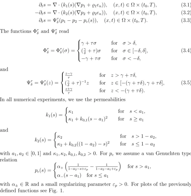
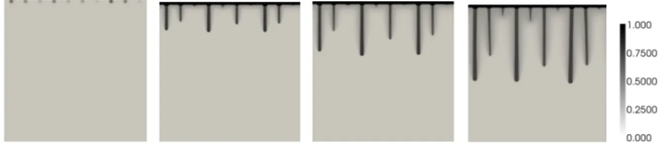
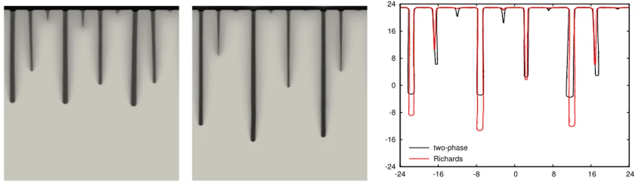
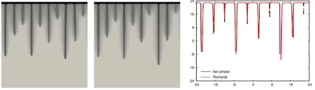
Numerical results. We include a numerical treatment of the two-phase flow equa- tions with hysteresis, (1.1)–(1.3). In agreement with the theoretical results, the finite- element scheme turns out to be stable; this holds true even though we include spatial and temporal adaptivity. We calculate solutions in a case that corresponds to the experimental set-up which is used to observe fingering effects in porous media. The presented model and the suggested discretization scheme provide numerical solutions that show gravity fingering in porous media. A description of the scheme and the investigated parameters is presented together with numerical results in Section 3.

1.1 Further literature on two-phase flow equations

Unfortunately, the name “two-phase flow” is slightly ambiguous, it is used for the above system, but also for the Richards equation. The Richards equation is the simplification of the above model that is obtained by assuming that the pressure of the second phase is constant, e.g. p₂ = 0, and by using only (1.1) instead of the set of equations (1.1)–(1.2). Even though also this simplified model describes the motion of two fluid phases, we will use the termtwo-phase flow equations only when we refer to system (1.1)–(1.2).

Results on the Richards equation. Even in the case without hysteresis, i.e.

with an algebraic relation p = p_c(s) instead of (1.3), the Richards equation is an interesting mathematical object due to the possible degeneracies k(s) = 0 for some s and p_c(s) → ±∞ for s tending to critical saturation values. Existence results are obtained e.g. in [2] and [3], uniqueness is treated e.g. in [20] and [12], the physical

outflow boundary conditions are treated e.g. in [1] and [23]. Regarding the numerical treatment of the Richards equation without hysteresis we mention [4, 21].

We want to highlight at this point the close connection between hysteresis effects and fingering in porous media; we refer to [25] and the references therein for exper- imental results on fingering. The analytical contributions of [20, 26] imply, loosely speaking, that fingering is not possible in the Richards equation without hysteresis.

On the other hand, it was shown theoretically in [24] and with numerical experiments in [17] that fingering can occur in the Richards equation if hysteresis is included.

The hysteresis relation (1.3), without the coupling to a partial differential equa- tion, poses already interesting questions regarding a functional analytic description, we refer to [28] for the corresponding discussion. In both cases, τ = 0 (rate- independent) and τ >0 (rate-dependent), the hysteresis relation may be considered as a functional relation s(t) = B(t, p|_[0,t]), where B maps the history of p to a value s(t), given initial values s0. We emphasize that, even in the equilibrium situation

∂_ts = 0, we cannot determine p(t) from s|_[0,t]. In this sense, the hysteresis relation cannot be inverted.

An existence result for the Richards equation with hysteresis was provided in [22] in the case that the partial differential equation is linear, i.e. in the case that k(.) is not depending on s and that p_c(.) is an affine function. In this situation, it was possible to treat the case τ = 0. Existence results for the nonlinear Richards equation with other hysteresis relations were obtained in [5] and [6] under very general assumptions, but not covering our model.

If the hysteresis model (1.3) is considered without the static part introduced by the sign function, the model can be re-written as a pseudo-parabolic equation.

Using this point of view, existence results are derived in [10] and [19], including some degeneracies of the coefficients. Closest to the contribution at hand is [17], where the nonlinear Richards equation with hysteresis was studied and an existence result was derived. The compactness result of Lemma 3.3 in [17] was crucial for the Richards equations and will be used again in the work at hand.

Results on the two-phase flow equation. The two-phase flow equations without hysteresis have been studied under the aspect of existence results in [13] and [16], uniqueness and regularity issues are treated in [13] and [14], outflow conditions in [18], maximum principles appear in [16] and [18]. Physical conditions across interior interfaces are investigated in [9] and [11]. We are not aware of any contribution that derives an existence result for the two-phase flow system with hysteresis. Regarding the numerical treatment of two-phase flow without hysteresis we refer to [7].

1.2 Assumptions and main result

In this subsection we fix the assumptions on the coefficient functions and formulate our main result. We consider non-linear, but non-degenerate permeabilities k_j, j = 1,2, and a strictly increasing, non-degenerate capillary pressure curve p_c. On the relaxation constant we assume positivity, τ > 0. We will construct solutions of the two-phase system with the specific hysteresis relation of (1.3), but the compactness result will exploit only the more general relation (1.4).

Initial and boundary conditions. The unknowns in the porous media model (1.1)–(1.3) are p₁, p₂, and s. Let Ω⊂Rⁿ such that

Ω is a Lipschitz domain and ∂Ω is decomposed as ∂Ω = ¯Γ1∪Σ¯1 = ¯Γ2∪Σ¯2 (1.5) with Γ_j∩Σ_j =∅two relatively open subsets of∂Ω forj = 1,2. We impose a Dirichlet condition for p_j on Σ_j and a Neumann condition for fluid j on Γ_j, for notational convenience we impose only no-flux conditions on Γ_j. We assume positivity of the Hausdorff measures, Hⁿ⁻¹(Σ_j) > 0 for j = 1,2. The Dirichlet conditions are given by two functions p_0,1, p_0,2 ∈ L²(0, T;H¹(Ω)). We prescribe initial values for the saturation by a function s₀ ∈L²(Ω).

Coefficient functions. Our assumptions on the coefficient functions are as follows.

For six positive numbers K_j, κ_j, κ⁰_j >0, j = 1,2, we assume

p_c∈C^0,1(R×Ω,R), γ ∈C^0,1(Ω,[0,∞)), (1.6) k_j ∈C(R×Ω,[κ_j, κ⁰_j]), kk_j(x, .)k_Lip(R,R) ≤K_j, for j ∈ {1,2}, x∈Ω. (1.7) We denote the Lipschitz constant of the capillary pressure by ρ := kpckLip and em- phasize that the Lipschitz continuity of p_c is assumed in x and s. We will always assume τ > 0 and use Φ : R×Ω → R,(ξ, x) 7→ τ ξ +γ(x)sign(ξ). Positivity of τ implies that Φ(., x) has a Lipschitz continuous inverse, we denote the inverse by Ψ(., x). This defines Ψ : R×Ω → R with 0 ≤ ∂_ζΨ(ζ, x) ≤ 1/τ for all ζ ∈ R. We finally assume that p_c has a positive primitive, i.e.

∃P_c∈C(R×Ω,R) with P_c(s, x)≥0, ∂_sP_c(s, x) =p_c(s, x) for all s∈R, x∈Ω.

(1.8) The gravity vectors g1, g2 ∈Rⁿ are constant vectors.

Weak form of equations (1.1) and (1.2). The first two evolution equations are expressed in the usual weak form. We say that s, p₁, p₂ ∈ L²(0, T;L²(Ω)) with

∂_ts ∈ L²(0, T;L²(Ω)) and ∇p₁,∇p₂ ∈ L²(0, T;L²(Ω)) solve (1.1)–(1.2) and the no- flux condition on Γ_j in the weak form if, for all test-functions ϕ_j ∈ L²(0, T;H¹(Ω)) with ϕ_j = 0 on Σ_j, there holds

Z

ΩT

k₁(s)[∇p₁+g₁]∇ϕ₁+ Z

ΩT

k₂(s)[∇p₂+g₂]∇ϕ₂ =− Z

ΩT

(ϕ₁−ϕ₂)∂_ts. (1.9) Main Theorem. Our main result concerns the existence of solutions to the non- degenerate two-phase flow equations.

Theorem 1.1 (Existence for the two-phase flow problem with hysteresis). Let the Lipschitz domain Ω⊂ Rⁿ with boundary parts Γ_j and Σ_j be as in (1.5). Let initial and boundary conditions be given by s₀ ∈L²(Ω) and p_0,1, p_0,2 ∈ L²(0, T;H¹(Ω)). Let the coefficients satisfy τ >0 and (1.6)–(1.8).

Then there exists a solution p₁, p₂ ∈ L²(0, T;H¹(Ω)) and s ∈ H¹(0, T;L²(Ω)) of the two-phase hysteresis system (1.1)–(1.3). More precisely, equations (1.1), (1.2), and the no-flux condition are satisfied in the weak form (1.9), the hysteresis relation (1.3) holds pointwise almost everywhere, initial and Dirichlet boundary conditions are satisfied in the sense of traces.

1.3 A priori estimates and solution concept

We start our analysis of system (1.1)–(1.3) by presenting the formal a priori estimates.

These indicate the natural norms and function spaces. At the same time, we will observe a lack of spatial regularity for the saturation variable s. It is this lack of compactness that makes the existence proof interesting.

We multiply (1.1) with p₁ −p_0,1 and (1.2) with p₂ −p_0,2 and integrate over Ω.

Adding the equations, we obtain (1.9) with ϕ_j =p_j−p_0,j. Inserting (1.3) gives Z

Ω

k₁(s)[∇p₁+g₁]∇[p₁ −p_0,1] + Z

Ω

k₂(s)[∇p₂ +g₂]∇[p₂−p_0,2]

=− Z

Ω

[(p₁−p₂)−p_0,1+p_0,2]∂_ts

∈ − Z

Ω

(p_c(s) +γsign(∂_ts) +τ ∂_ts)∂_ts+ Z

Ω

(p_0,1−p_0,2)∂_ts.

By assumption (1.8), the monotone function p_c has a convex, positive primitive P_c. Integration over t ∈ [0, T] and application of the Cauchy-Schwarz and the Poincar´e inequality yields in the standard fashion the estimate

Z

Ω

P_c(s) t=T

+ Z

ΩT

k₁(s)|∇p₁|²+k₂(s)|∇p₂|²+γ|∂_ts|+τ|∂_ts|² ≤C₀, (1.10) where the constant C₀ depends on the data g_j, p_0,j, s₀, on τ and on the other sys- tem constants introduced before (1.6). We exploited that p_c is Lipschitz continuous and that, as a consequence, Pc has at most quadratic growth in s. The domain of integration is Ω_T = Ω×(0, T).

Variational weak solutions

In the solution concept of Theorem 1.1 we demand that relation (1.3) holds for almost all (x, t) ∈Ω_T. In order to verify this condition, it is convenient to use additionally the notion of variational weak solutions.

Definition 1.2 (Variational weak solution). Let (s, p₁, p₂) be a triple of functions with

s ∈L^∞(0, T;L²(Ω)), ∂_ts∈L²(0, T;L²(Ω)), p₁, p₂ ∈L²(0, T;H¹(Ω)), (1.11) satisfying, in the sense of traces, the initial condition s = s₀ on Ω× {0} and the boundary conditions p_j =p_0,j on Σ_j ×(0, T). The triple is called a variational weak solution of the two-phase equation if the following three conditions are satisfied.

1. The evolution equations (1.1)–(1.2) and the no-flux conditions are satisfied in the weak sense of (1.9).

2. The relation p₁(x, t)−p₂(x, t)−p_c(s(x, t), x)−τ ∂_ts(x, t)∈[−γ(x), γ(x)] holds for almost every (x, t)∈Ω_T.

3. The variational inequality 0≥

Z

ΩT

(p_c(s)−p_0,1+p_0,2)∂_ts+ Z

ΩT

τ|∂_ts|²+γ|∂_ts|

+ Z

ΩT

k₁(s)[∇p₁+g₁]∇[p₁−p_0,1] + Z

ΩT

k₂(s)[∇p₂+g₂]∇[p₂−p_0,2]

(1.12)

is satisfied.

Lemma 1.3. Let(s, p1, p2)be a variational weak solution as in Definition 1.2. Then (1.3) is satisfied almost everywhere. In particular, (s, p₁, p₂) is a solution of (1.1)–

(1.3) as described in Theorem 1.1.

Proof. We only have to show that (1.3) holds almost everywhere. For weak solutions, the two distributions∇·(kj(s)[∇pj+gj]) =±∂tsare actuallyL²(ΩT)-functions, hence we can perform an integration by parts in the last two integrals of (1.12). Then the inequality (1.12) simplifies to

0≥ Z

ΩT

(p_c(s)−p₁+p₂)∂_ts+ Z

ΩT

τ|∂_ts|²+γ|∂_ts| . We write this as

Z

ΩT

γ|∂_ts| ≤ Z

ΩT

[p₁−p₂−p_c(s)−τ ∂_ts]∂_ts.

By property 2 of variational weak solutions, the integrand on the right hand side satisfies [p₁−p₂−p_c(., s)−τ ∂_ts]∂_ts≤γ|∂_ts|almost everywhere, and is therefore smaller or equal to the integrand on the left hand side. Since the integral inequality is in the opposite direction, the integrands must coincide, [p₁−p₂−p_c(., s)−τ ∂_ts]∂_ts=γ|∂_ts|

holds almost everywhere. This, together with property 2 of variational weak solutions, implies the pointwise inclusion (1.3).

We see that Theorem 1.1 is shown once that we prove the existence of a variational weak solution as in Definition 1.2.

2 Discrete system and proof of the main theorem

2.1 The discrete system

Our next aim is to define a Galerkin scheme such that the original equations (1.1)–

(1.3) are approximated by a system of ordinary differential equations. With this aim we introduce a space-discretization with parameter h > 0. We recall that three positive (and possibly small) physical parameters appear in the equations: the num- bers κ₁, κ₂ > 0 are lower bounds for the permeabilities and τ > 0 is the time delay parameter.

In the case of a vanishing time delay, τ = 0, the play-type relation (1.3) can be written with the multi-valued function Φ⁰(σ) := γsign(σ) asp₁−p₂ ∈p_c(s)+Φ⁰(∂_ts).

In the general caseτ ≥0 and withγ =γ(x) we use Φ^τ := Φ⁰+τid, or, more precisely,

Φ^τ(σ, x) :=







[−γ(x), γ(x)] for σ= 0 γ(x) +τ σ for σ >0

−γ(x) +τ σ for σ <0.

(2.1)

With this choice, (1.3) can be written as p₁−p₂ ∈ p_c(s) + Φ^τ(∂_ts); we suppress the dependence onxwhenever possible. We denote the inverse by Ψ^τ(., x) := (Φ^τ(., x))⁻¹. The inverse Ψ^τ : R×Ω → R is multivalued only in the case τ = 0. For positive τ, the function Ψ^τ is single-valued with maximal slope τ⁻¹. In this sense, τ >0 can be regarded as a regularization of the system.

Spatial discretization. We next discretize the spatial domain Ω. In order to simplify notation, we describe the method for the case that the domain Ω is polygonal;

in the case of a general Lipschitz domain, it poses no problem to use boundary elements that are not simplices.

LetTh be a triangulation of Ω, decomposing Ω into finitely many simplicesA∈ Th. Let h > 0 be an upper bound for the diameter of all elements of T_h. We denote by Ω_h ={x₁, . . . , x_N} a suitable subset ofN points, such that we can associate to every triangle A∈ Th a uniquely determined point x∈ Ωh ∩A. The set of points (xk)k≤N

defines a projection X^h : Ω → Ω_h. The map X^h can also be used to define an invertible map that identifies R^N with piecewise constant functions (defined almost everywhere),

J :R^N ≡ {f : Ω_h →R} −→ {fˆ: Ω→R piecewise constant}=:P₀(Ω,T_h), (2.2) by (J f)(x) =f(X^h(x)) for almost every x∈Ω. We will furthermore use the L²(Ω)- orthogonal projection P := P_h : L²(Ω) → L²(Ω) to the space of piecewise con- stant functions P0(Ω,Th). A continuous function on Ω can be discretized with the help of X^h : Ω → Ω_h. To give an example, given γ = γ(x), we can restrict to the relevant corners and consider γ|_Ωh, and correspondingly the piecewise constant parameter function γ^h(x) := J(γ|Ω_h)(x) = γ(X^h(x)). Accordingly, we define the piecewise constant (in x) coefficient function p^h_c(s, x) := p_c(s, X^h(x)) and its prim- itive P_c^h(s, x) = P_c(s, X^h(x)) with ∂_sP_c^h(s, x) = p^h_c(s, x). Analogously, the function Φ^τ(σ, x) of (2.1) is discretized in space to Φ^τ_h(σ, x) := Φ^τ_h(σ, X^h(x)) and its inverse (in the variable σ) is Ψ^τ_h(., x) = (Φ^τ_h(., x))⁻¹. With this notation, we can now define the Galerkin scheme.

Definition 2.1 (Galerkin scheme). Our unknowns are piecewise constant functions p^h_j : Ω×[0, T]→R, j = 1,2 and s^h : Ω×[0, T]→R, identified with maps p^h₁, p^h₂, s^h : [0, T]→ P₀(Ω,T_h). We demand, for almost every x∈Ωand almost every t∈(0, T),

∂ts^h(x, t) =Ψ^τ_h(p^h₁(x, t)−p^h₂(x, t)−p^h_c(s^h, x)),

s^h(x,0) =(P_hs₀)(x), (2.3)

where we suppressed the explicit dependence of Ψ^τ_h on x. The pressures p^h₁ and p^h₂ are reconstructed from s^h as follows. We solve with two functions p˜^h_j ∈ H¹(Ω,R),

j = 1,2, in a weak sense the elliptic system

−∇ · k₁(s^h, x)(∇˜p^h₁ +g₁)

= Ψ^τ_h p_c(s^h, x)−P_h[˜p^h₁ −p˜^h₂]

in Ω (2.4)

−∇ · k₂(s^h, x)(∇˜p^h₂ +g₂)

=−Ψ^τ_h p_c(s^h, x)−P_h[˜p^h₁ −p˜^h₂]

in Ω (2.5)

˜

p^h_j(·, t) = p_0,j(·, t) on Σ_j for j = 1,2, (2.6) for all t∈ [0, T], with no-flux conditions on Γ_j. The discrete pressures are recovered by a projection, p^h_j =P_hp˜^h_j for j = 1,2.

For later use we note that the evolution equation in (2.3) can also be written as Φ^τ_h(∂_ts^h) = Φ⁰_h(∂_ts^h(x, t)) +τ ∂_ts^h 3p^h₁ −p^h₂ −p^h_c(s^h). (2.7) We note that Φ^τ_h and Φ⁰_h depend via γ^h(x) also in a direct way onx∈Ω.

2.2 Well-posedness of the Galerkin scheme

Our aim is to prove that (2.3) is an ordinary differential equation for s^h : [0, T] → P₀(Ω,T_h). With this perspective, we want to show that the system (2.4)–(2.6) defines a Lipschitz-continuous map s^h 7→ (p^h₁, p^h₂) = (P_hp˜^h₁, P_hp˜^h₂). Once this is shown, we have verified that the Galerkin scheme consists of the ordinary differential equation (2.3) (the image spaceP₀(Ω,T_h) is finite dimensional) with an intricate, but Lipschitz continuous right hand side.

The aim of the next lemma is precisely this analysis of the stationary system (2.4)–(2.6). We write ˜p^h_j = p_0,j +u_j for j = 1,2, such that (2.4) and (2.5) read, omitting the h-dependence of the function s,

−∇ ·(k₁(s)∇u₁) =Ψ^τ_h(p_c(s)−P_h(u₁−u₂)−P_h(p_0,1−p_0,2)) +∇ ·(k₁(s)(∇p_0,1+g₁)),

−∇ ·(k2(s)∇u2) =−Ψ^τ_h(pc(s)−Ph(u1−u2)−Ph(p0,1−p0,2)) +∇ ·(k₂(s)(∇p_0,2+g₂)).

We introduce some abbreviations. Let f :R×R×Ω→R be the function

f(s, z, x) :=−Ψ^τ_h(p_c(s, x)−z−P_h(p_0,1−p_0,2)(x), x). (2.8) Then s 7→f(s, z, x) is Lipschitz continuous with Lipschitz constant ρτ⁻¹. The map z 7→ f(s, z, x) is monotonically non-decreasing and Lipschitz continuous with Lips- chitz constant τ⁻¹. In the following, we suppress the explicit x-dependece of Ψ^τ_h. We use F :L²(Ω)×L²(Ω)→L²(Ω),

F(s, z)(x) :=f(s(x), z(x), x). (2.9) Later on, we will insertP_h(u₁−u₂) for the variablez. With this choice, the expression f(s, z, x) coincides, up to signs, with the first part in the right hand sides of (2.4) and (2.5). To abbreviate also the other lower order terms, we use, for j = 1,2, the map ¯G_j :L²(Ω)→L²(Ω),

G¯_j(s)(x) := k_j(s(x), x)(∇p_0,j(x) +g_j). (2.10) We intend to use piecewise constant functionss, z ∈ P₀(Ω,T_h) and note that functions such as p_c(s, x), F(s, z), or ¯G_j(s) are not piecewise constant functions in general.

Lemma 2.2 (Local existence result for the discrete stationary system). Let the data Ω, p_c, k_j, g_j, p_0,j and τ >0 satisfy (1.5)–(1.8). Let the hysteresis function Ψ^τ_h and the projection P_h be as described before Definition 2.1. Let F and G¯_j be as in (2.8)–

(2.10). Then there exists a positive number h0 >0 such that the following statements hold.

Existence. Let h ∈ (0, h₀) and S ∈ L^∞(Ω) be arbitrary. We consider the spaces H_0,j(Ω) := {u_j ∈H¹(Ω) :u_j = 0 on Σ_j} and search for solutions u = (u₁, u₂) in the product space u ∈ H_0,1(Ω)×H_0,2(Ω). For arbitrary right hand sides G_j ∈ H_0,j(Ω)⁰, j = 1,2, there exist a unique weak solution u= (u₁, u₂) of

−∇ ·(k₁(S)∇u₁) =−F(S, P_h(u₁ −u₂)) +G₁

−∇ ·(k₂(S)∇u₂) =F(S,(P_h(u₁−u₂)) +G₂ (2.11) in Ω, with a weak no-flux conditionn·[∇(p_0,j+u_j) +g_j] = 0 on Γ_j.

Lipschitz continuity. For every R > 0 there exists a positive constant C = C(R) such that the following holds. Lets,˜s∈L^∞(Ω)withksk∞,k˜sk∞≤R. Letu= (u1, u2) be a solution of (2.11) for S =s and G_j :ϕ7→ −R

ΩG¯_j(s)∇ϕ. Let u˜= (˜u₁,u˜₂) be a solution of (2.11) for S = ˜s and G_j :ϕ7→ −R

ΩG¯_j(˜s)∇ϕ. Then

ku−uk˜ _H¹_(Ω,R²₎ ≤Cks−˜sk_L^∞_(Ω). (2.12) Proof. We search for solutions in the product space H := H_0,1(Ω)×H_0,2(Ω). The space H is a Hilbert space with the norm of H¹(Ω)×H¹(Ω) and the dual space is H⁰ =H_0,1(Ω)⁰×H_0,2(Ω)⁰.

Step 1: Re-formulation of the system. In a later step, we want to perform a continuity method. We therefore generalize the system slightly and consider, for λ ∈[0,1], the following system for u= (u1, u2)∈H,

−∇ ·(k1(S, x)∇u1) =−λF(S, Ph(u1−u2)) +G1

−∇ ·(k₂(S, x)∇u₂) =λF(S, P_h(u₁−u₂)) +G₂ (E_λ) in the weak form and with the same no-flux condition. With this choice of (E_λ), problem (E₁) for λ = 1 coincides with the original problem (2.11). On the space H we define a bilinear form B_S :H×H→R as

B_S[u, ϕ] :=

Z

Ω

k₁(S, x)∇u₁(x)∇ϕ₁(x) +k₂(S, x)∇u₂(x)∇ϕ₂(x)dx

foru= (u₁, u₂), ϕ= (ϕ₁, ϕ₂)∈H. The pairG:= (G₁, G₂) satisfiesG∈H⁰. Equation (E_λ) now reads

BS[u, ϕ] =−λ Z

Ω

F(S, Ph(u1−u2))(ϕ1−ϕ2) +hG, ϕi (2.13) for all ϕ∈H; here h·,·i denotes the duality pairing between H⁰ and H.

Step 2: A priori estimates. We useϕ=uin (2.13). Poincar´e’s inequality and the positiviy of k₁, k₂ imply the coercivity ofB_S and we obtain with c >0

ckuk²_H ≤ Z

Ω

k₁(S)|∇u₁|²+k₂(S)|∇u₂|² =B_S[u, u]

=−λ Z

Ω

F(S, Ph(u1−u2))(u1−u2) +hG, ui.