Stable finite element approximations of two-phase flow with soluble surfactant

Universit¨ at Regensburg Mathematik

Stable finite element approximations of two-phase flow with soluble surfactant

John W. Barrett, Harald Garcke and Robert N¨ urnberg

Preprint Nr. 14/2014

Stable Finite Element Approximations of Two-Phase Flow with Soluble Surfactant

John W. Barrett

Harald Garcke

Robert N¨ urnberg

Abstract

A parametric finite element approximation of incompressible two-phase flow with soluble surfactants is presented. The Navier–Stokes equations are coupled to bulk and surfaces PDEs for the surfactant concentrations. At the interface adsorption, desorption and stress balances involving curvature effects and Marangoni forces have to be considered. A parametric finite element approximation for the advection of the interface, which maintains good mesh properties, is coupled to the evolv- ing surface finite element method, which is used to discretize the surface PDE for the interface surfactant concentration. The resulting system is solved together with standard finite element approximations of the Navier–Stokes equations and of the bulk parabolic PDE for the surfactant concentration. Semidiscrete and fully discrete approximations are analyzed with respect to stability, conservation and ex- istence/uniqueness issues. The approach is validated for simple test cases and for complex scenarios, including colliding drops in a shear flow, which are computed in two and three space dimensions.

Key words. incompressible two-phase flow, soluble surfactants, finite elements, front tracking, ALE-ESFEM

1 Introduction

Surface active agents, also called surfactants, are among the most widely used molecules in industry. They may act as detergents, wetting agents, emulsifiers, foaming agents and dispersants. The reason for these many applications is that soluble surfactants can have a pronounced effect on the interface and, hence also, on the evolution in a two-phase flow. In particular, surfactants influence the surface tension at the interface, and local inhomogeneities lead to Marangoni effects. In situations where the surfactant is soluble in one or in both of the two bulk phases, the adsorption and desorption of surfactants at the interface has to be taken into account. This means surfactant molecules can attach

†Department of Mathematics, Imperial College London, London, SW7 2AZ, UK

‡Fakult¨at f¨ur Mathematik, Universit¨at Regensburg, 93040 Regensburg, Germany

to and detach from the interface, and the corresponding mass balances on the interface and in the bulk have to be taken into account. The fundamental transport mechanisms for surfactants are diffusion in the bulk phases and on the interface, and advection with the underlying fluid velocity.

Adsorption of surfactants to the interface decreases the surface tension, which makes it easier for the interface to deform. It also can be observed, see e.g. the numerical exper- iments in Section 6, that an interface moves towards regions with a high bulk surfactant concentration. The presence of surfactants typically decreases the rise velocity of bubbles.

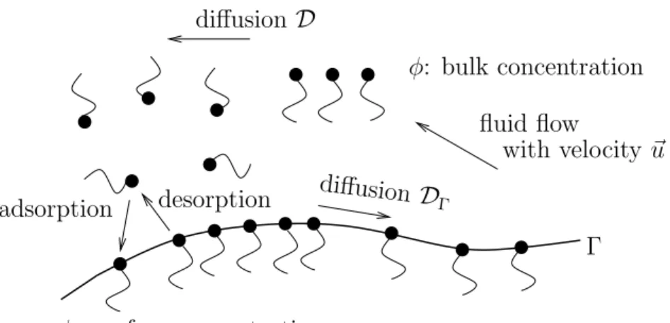
The reason for this is that Marangoni stresses at the interface imply that the shear free condition at the interface no longer holds, and hence the drag force on the bubble in- creases. In particular, the rise velocity of a bubble is reduced, and this effect can be used to maximize the contact time between different fluid phases, which can be important to influence the transfer of chemical components. These phenomena demonstrate that the interplay between the fluid velocity and the bulk and surface surfactant concentrations is multifaceted. Due to this versatile interaction it is often difficult to identify the sources for the different phenomena from experiments alone. It is hence important to have re- liable numerical methods for this complex problem at hand in order to obtain a better understanding of the interdependence of fluid flow, adsorption, desorption, advection, Marangoni effects and diffusion, see Figure 1 for a schematic description of the different quantities and transport processes.

diffusion D

φ: bulk concentration

adsorption desorption diffusion D_Γ

ψ: surface concentration

Γ fluid flow

with velocity ~u

Figure 1: The different quantities and transport phenomena in the bulk and at the inter- face are schematically illustrated.

In order to mathematically describe the complex physics illustrated in Figure 1, one has to solve the following equations.

• The incompressible Navier–Stokes equations in both phases, see (2.3a–c).

• An advection-diffusion equation for the bulk surfactant concentration in either one or in both phases, see (2.8a).

• A parabolic partial differential equation on the evolving interface describing the conservation of bulk surfactant. Here a source term stemming from desorption and adsorption of surfactants has to be taken into account, see (2.8b) and Figure 1.

• An equilibrium of force equation on the interface, which includes curvature and Marangoni effects, see (2.5a).

• An additional interface equation taking the surface thermodynamics into account.

Depending on whether the interface kinetics are slow or fast, this either results in a condition relating the bulk fluxes to differences of chemical potentials, or it leads to the chemical potentials having to be equal, see (2.13) and (2.15). The latter condition contains Henry’s law (2.17) as a special case.

In addition,

• the interface has to be advected with a normal velocity which equals the normal part of the fluid velocity, see (2.5b).

Although the overall problem has many applications, not many analytical results exist for this problem. An energy inequality for the insoluble case, which we are also going to use, has been derived by Garcke and Wieland (2006). Bothe and Pr¨uss (2010) used energy methods and semigroup theory to study the stability of equilibria in the soluble case. Garckeet al. (2014) introduced a diffuse interface model to describe two-phase flow with soluble surfactants for which an energy inequality can be shown. Moreover, by using matched asymptotic expansions they could show that a novel sharp interface model can be recovered, which also satisfies an energy law. We refer to Section 2 for the precise details of this sharp interface model, which has already been outlined above.

In contrast, over the years many papers presenting numerical methods and computa- tions for interfacial flows with soluble surfactants have appeared. Let us briefly mention the methods that have been used by different groups. Renardyet al.(2002) and Alke and Bothe (2007) used the volume of fluid (VOF) method, which approximates the character- istic function of one of the phases. The level set method, which describes the interface as the level set of a function, was considered in the work of Xuet al.(2013). Numerical com- putations based on diffuse interface models have been presented by Liu and Zhang (2010), Teigenet al.(2011), Engblomet al.(2013) and Garckeet al.(2014). The immersed bound- ary method has been used by Laiet al.(2008) and Chen and Lai (2014). A front tracking method for soluble surfactants has been introduced by Muradoglu and Tryggvason (2008) and Tasoglu et al. (2008). In addition we mention the arbitrary Lagrangian–Eulerian approach of Ganesan and Tobiska (2012), the segment projection method of Khatri and Tornberg (2014) and the hybrid method studied in Booty and Siegel (2010) and Xu et al.

(2013). For more references and an introduction to numerical methods for two-phase flow we refer to the book by Groß and Reusken (2011).

In this paper we adapt the approach of Barrett et al. (2014, 2013b) to numerically solve the governing equations for soluble surfactants at fluid interfaces. In particular, we

consider the system with the novel free boundary condition in Garcke et al. (2014) that allows for a stability estimate. For a particular instance of this model, where the bulk surfactant concentration is assumed to be continuous across the interface, we are able to prove a stability estimate for our semidiscrete finite element approximation. To our knowledge, this is the first stability result for a numerical approximation of two-phase flow with soluble surfactant in the literature. In addition, the numerical method introduced by the present authors ensures good mesh properties, i.e. equidistribution of interface mesh pointsin 2d, see Barrettet al.(2007), andconformal polyhedral surfacesin 3d, see Barrett et al. (2008). In addition, a simple XFEM strategy ensures discrete volume conservation and often mass conservation and stability estimates can be shown. The mesh properties also make a reliable computation of the PDE on the evolving interface possible. To solve this PDE we use the evolving surface finite element method (ESFEM) of Dziuk and Elliott (2007), see also the ALE-ESFEM approach of Elliott and Styles (2012).

The remainder of the paper is organized as follows. In Section 2 we state the governing equations. Two alternative weak formulations for different models of two-phase flow with soluble surfactant are introduced in Section 4. Here we consider a two-sided model (i) with the relaxation condition (2.13), as well as a global model (ii), where the soluble surfactant concentration is assumed to be continuous across the interface. The natural semidiscrete continuous-in-time finite element approximations based on these formulations are presented in Section 4, together with stability proofs for the approximations of model (ii). Fully discrete analogues are discussed in Section 5, with numerical results shown in Section 6. Here we show numerical simulations for colliding drops in shear flow and for rising bubbles, and we also present computations for radially symmetric solutions for a simple test problem involving adsorption and desorption, which underline the accuracy of our numerical method. The details for the employed radially symmetric solutions are discussed in the Appendix.

2 Governing equations

We will now introduce the sharp interface model for two-phase flow with surfactants which we plan to numerically approximate.

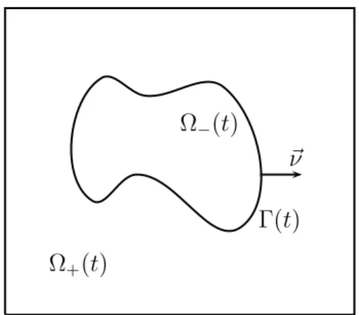
Let Ω⊂R^d be a given domain, where d= 2 ord= 3. We now seek a time dependent interface (Γ(t))t∈[0,T], Γ(t)⊂ Ω, which for all t∈ [0, T] separates Ω into a domain Ω+(t), occupied by one phase, and a domain Ω₋(t) := Ω\ Ω₊(t), which is occupied by the other phase. Here the phases could represent two different liquids, or a liquid and a gas.

Common examples are oil/water or water/air interfaces. See Figure 2 for an illustration.

For later use, we assume that (Γ(t))_t∈[0,T] is a sufficiently smooth evolving hypersurface without boundary that is parameterized by ~x(·, t) : Υ → R^d, where Υ ⊂ R^d is a given reference manifold, i.e. Γ(t) =~x(Υ, t). Then

V(~z, t) :=~ ~xt(~q, t) ∀ ~z=~x(~q, t)∈Γ(t) (2.1) defines the velocity of Γ(t), and ~V. ~ν is the normal velocity of the evolving hypersurface

~ν

Γ(t) Ω₋(t)

Ω₊(t)

Figure 2: The domain Ω in the case d= 2.

Γ(t), where~ν(t) is the unit normal on Γ(t) pointing into Ω+(t). Moreover, we define the space-time surface

GT := [

t∈[0,T]

Γ(t)× {t}. (2.2)

Let ρ(t) = ρ+X_Ω+(t) +ρ−X_Ω−(t), with ρ± ∈ R_>0, denote the fluid densities, where here and throughout XA defines the characteristic function for a set A. Denoting by

~u: Ω×[0, T]→R^d the fluid velocity, by σ : Ω×[0, T]→R^d×d the stress tensor, and by f~: Ω×[0, T]→R^d a possible forcing, the incompressible Navier–Stokes equations in the two phases are given by

ρ(~ut+ (~u .∇)~u)− ∇. σ =f~:=ρ ~f1+f~2 in Ω±(t), (2.3a)

∇. ~u= 0 in Ω±(t), (2.3b)

[~u]⁺₋ =~0 on Γ(t), (2.3c)

~u=~0 on∂1Ω, (2.3d)

~u . ~n = 0, σ ~n.~t = 0 ∀~t∈ {~n}^⊥ on∂2Ω, (2.3e) where ∂Ω =∂1Ω∪∂2Ω, with ∂1Ω∩∂2Ω =∅, denotes the boundary of Ω with outer unit normal~n and{~n}^⊥ :={~t∈R^d:~t. ~n = 0}. Hence (2.3d) prescribes a no-slip condition on

∂1Ω, while (2.3e) prescribes a free-slip condition on ∂2Ω. In addition, the stress tensor in (2.3a) is defined by

σ=µ(∇~u+ (∇~u)^T)−p Id= 2µ D(~u)−p Id , (2.4) where Id ∈ R^d×d denotes the identity matrix, D(~u) := ¹₂(∇~u + (∇~u)^T) is the rate-of- deformation tensor, p: Ω×[0, T]→ R is the pressure and µ(t) = µ+XΩ+(t)+µ−XΩ−(t), with µ± ∈ R_>0, denotes the dynamic viscosities in the two phases. On the free surface Γ(t), the following conditions need to hold:

[σ ~ν]⁺₋ =−γ(ψ)κ~ν − ∇sγ(ψ) on Γ(t), (2.5a)

V~. ~ν =~u . ~ν on Γ(t), (2.5b)

where γ ∈C¹([0, ψ∞)), with ψ∞>0 and

γ^′(r)<0 ∀ r ∈[0, ψ_∞), (2.6) denotes the surface tension which depends on the interfacial surfactant densityψ :GT → (0, ψ∞), recall (2.2), and ∇s denotes the surface gradient on Γ(t). In addition, κ denotes the mean curvature of Γ(t), i.e. the sum of the principal curvatures of Γ(t), where we have adopted the sign convention that κ is negative where Ω−(t) is locally convex. In particular, on letting id denote the identity function in~ R^d, it holds that

∆sid =~ κ~ν =:~κ on Γ(t), (2.7) where ∆s=∇s.∇s is the Laplace–Beltrami operator on Γ(t), with ∇s. denoting surface divergence on Γ(t). Moreover, as usual, [~u]⁺₋ :=~u+−~u−and [σ ~ν]⁺₋ :=σ+~ν−σ−~ν denote the jumps in velocity and normal stress across the interface Γ(t). Here and throughout, we employ the shorthand notation ~v_± :=~v|_Ω±(t) for a function ~v : Ω×[0, T]→ R^d; and similarly for scalar and matrix-valued functions. In this paper we consider surfactant that is soluble in the bulk phases. We denote the surfactant’s bulk densities by φ±, and the interfacial surfactant density by ψ, see above. The surfactant is transported by the surrounding fluid and, taking also diffusion into account, this can be modelled by

∂tφ_±+~u .∇φ_±− ∇.(D_±∇φ_±) = 0 in Ω_±(t), (2.8a)

∂_t^•ψ+ψ∇s.~u− ∇s.(D_Γ∇sψ) = [D ∇φ . ~ν]⁺₋ on Γ(t), (2.8b)

∇φ+. ~n +λ+(φ+−g+) = 0 on∂Ω, (2.8c) where D± ∈ R_≥0 and DΓ ∈ R_≥0 are diffusion coefficients, and where [D ∇φ . ~ν]⁺₋ :=

D₊∇φ+. ~ν − D₋∇φ−. ~ν. In addition, λ+ ≥ 0 and g+ > 0 in the Robin boundary conditions (2.8c) are space-dependent parameters, and for notational convenience we also define λ−=g−= 0. Moreover,

∂_t^•ζ =ζt+~u .∇ζ ∀ ζ ∈H¹(GT) (2.9) denotes the material time derivative of ζ on Γ(t). Here we stress that for ζ ∈ H¹(GT) the derivative in (2.9) can be computed by extending ζ to a neighbourhood of GT. The quantity ∂_t^•ζ is well-defined, and depends only on the values of ζ on GT, even though ζt

and∇ζ do not make sense for a function onGT; see e.g. Dziuk and Elliott (2013, p. 324).

In order to formulate the necessary matching conditions that ψ andφ±need to satisfy on Γ(t), we introduce the surface energy function F, which satisfies

γ(r) =F(r)−r F^′(r) ∀ r ∈(0, ψ∞), (2.10a) and

limr→0r F^′(r) =F(0)−γ(0) = 0. (2.10b) This means in particular that

γ^′(r) =−r F^′′(r) ∀ r ∈(0, ψ∞). (2.11)

It immediately follows from (2.11) and (2.6) that F ∈C([0, ψ∞))∩C²(0, ψ∞) is convex.

Typical examples for γ and F are given by

γ(r) = γ0(1−β r), F(r) =γ0[1 +β r(lnr−1)], ψ∞ =∞, (2.12a) which represents a linear equation of state, and by

γ(r) =γ0

h1 +β ψ∞ ln 1− _ψ^r

∞

i, F(r) = γ0

h1 +β

r ln_ψ ^r

∞−r +ψ∞ ln^ψ∞_ψ^−r

∞

i,

(2.12b) the so-called Langmuir equation of state, whereγ₀, β ∈R_>0 are further given parameters, see e.g. Ravera et al. (2000).

Defining the relaxation parameters α± ∈R_>0, the missing interface condition is

±α_±D_±∇φ_±. ~ν =−[F^′(ψ)−G^′_±(φ_±)] on Γ(t), (2.13) which couplesψandφ±. This equation relates the bulk fluxes to differences of the chemical potentials F^′(ψ), G^′(φ+), G^′(φ−), see Garcke et al. (2014). Here G±∈C(R_≥0)∩C²(R_>0) are bulk free energy densities that satisfy

G^′′_±(s)≥0 ∀ s∈R_>0. (2.14)

We observe thatα± ∈R_>0relax the so-called instantaneous conditions (2.13) withα± = 0, which yield an algebraic relationship between ψ and φ± on Γ(t), namely

F^′(ψ) =G^′₋(φ₋) =G^′₊(φ₊) on Γ(t). (2.15) A typical example for G_± is

G±(r) =γ0β r[ln(θ±r)−1], (2.16) where θ± ∈ R_>0. In this case the identity G^′₋(φ−) = G^′₊(φ+) in (2.15) leads to Henry’s law

φ₊=KHφ₋, (2.17)

with the Henry constant KH =θ−/θ+. In order to make (2.13) well-defined, we assume from now on, and throughout this paper, that

ψ(·, t)∈(0, ψ∞) and φ±(·, t)>0 on Γ(t). (2.18) We remark that on combining (2.12b) with (2.16), the interface condition (2.13) for the outer phase, say, reduces to

α+D+∇φ+. ~ν =−[F^′(ψ)−G^′₊(φ+)]

=γ0β lnθ+φ+(ψ∞−ψ) ψ

≈γ0β

θ+φ+(ψ∞−ψ)

ψ −1

= γ0β

ψ [θ+φ+(ψ∞−ψ)−ψ], (2.19)

where we have used the approximation ln(1 +r) ≈ r for |r| ≪ 1. Clearly the condition (2.19) is closely related to conditions proposed by other authors. See e.g. the conditions in Muradoglu and Tryggvason (2008), Alke and Bothe (2009), Teigenet al.(2011), Ganesan and Tobiska (2012, (5)), Xu et al. (2013), and the kinetic condition in Diamant and Andelman (1996, (2.14)); see also Diamant and Andelman (1996, (23)).

Generalizing the work of Diamant and Andelman (1996) the model (2.3a-e), (2.4), (2.5a,b), (2.8a-c) was supplemented with (2.13) in a paper by Garckeet al.(2014). We will see in Subsection 6.1.1 that close to the equilibrium this model is related to the classical equilibrium condition (2.19) studied by the above authors. The important feature of (2.13) is that it allows for an energy inequality, see Garcke et al. (2014) and (3.17).

The system (2.3a–e), (2.4), (2.5a,b), (2.8a–c), (2.13) is closed with the initial conditions Γ(0) = Γ0, ψ(·,0) =ψ0 on Γ0, φ±(·,0) =φ±,0 in Ω±(0),

~u(·,0) =~u₀ in Ω, (2.20)

where Γ0 ⊂Ω, ~u0 : Ω→ R^d, with ∇. ~u0 = 0, φ±,0 : Ω±(0) →R_≥0, and ψ0 : Γ0 →(0, ψ∞) are given initial data.

3 Weak formulations

Before introducing our finite element approximations, we will state an appropriate weak formulation. With this in mind, we introduce the function spaces

U:={ϕ~ ∈[H¹(Ω)]^d:ϕ~=~0 on ∂1Ω, ~ϕ . ~n = 0 a.e. on ∂2Ω}, P:=L²(Ω), b

P:={η ∈P: Z

Ω

η dL^d= 0}, V:=L²(0, T;U)∩H¹(0, T; [L²(Ω)]^d), S:=H¹(GT), T:=L²(0, T;H¹(Ω))∩H¹(0, T;H⁻¹(Ω)), T_± :=H¹(Q_T,±),

where, similarly to (2.2), we define

Q_T,± := [

t∈[0,T]

Ω±(t)× {t}.

Let (·,·), (·,·)Ω±(t) and h·,·iΓ(t) denote the L²–inner products on Ω, Ω±(t) and Γ(t), re- spectively.

We recall from Barrett et al. (2014) that it follows from (2.3b–e) and (2.5b) that (ρ(~u .∇)~u, ~ξ) = ¹₂

(ρ(~u .∇)~u, ~ξ)−(ρ(~u .∇)ξ, ~u)~ −D

[ρ]⁺₋~u . ~ν, ~u . ~ξE

Γ(t)

∀ ξ~∈[H¹(Ω)]^d (3.1)

and

d

dt(ρ ~u, ~ξ) = (ρ ~ut, ~ξ) + (ρ ~u, ~ξt)−D

[ρ]⁺₋~u . ~ν, ~u . ~ξE

Γ(t) ∀ ~ξ∈V, respectively. Therefore, it holds that

(ρ ~ut, ~ξ) = ¹₂ d

dt(ρ ~u, ~ξ) + (ρ ~ut, ~ξ)−(ρ ~u, ~ξt) +D

[ρ]⁺₋~u . ~ν, ~u . ~ξE

Γ(t)

∀ ~ξ∈V,

which on combining with (3.1) yields that (ρ[~ut+ (~u .∇)~u], ~ξ)

= ¹₂ d

dt(ρ ~u, ~ξ) + (ρ ~ut, ~ξ)−(ρ ~u, ~ξt) + (ρ,[(~u .∇)~u]. ~ξ−[(~u .∇)~ξ]. ~u)

∀ ξ~∈V. (3.2) Moreover, it holds on noting (2.3e) and (2.5a) that for all ξ~∈U

Z

Ω+(t)∪Ω−(t)

(∇. σ). ~ξdL^d =−2 (µ D(~u), D(~ξ)) + (p,∇. ~ξ) +D

γ(ψ)κ~ν+∇sγ(ψ), ~ξE

Γ(t) . (3.3) Similarly to (2.9) we define the following time derivative that follows the parameteri- zation~x(·, t) of Γ(t), rather than ~u. In particular, we let

∂_t^◦ζ =ζt+V~.∇ζ ∀ ζ ∈S, (3.4) recall (2.1). Here we stress once again that this definition is well-defined, even though ζt

and ∇ζ do not make sense separately for a function ζ ∈S. On recalling (2.9) we obtain that

∂_t^◦ =∂_t^• if V~ =~u on Γ(t). (3.5) We note that the definition (3.4) differs from the definition of ∂^◦ in Dziuk and Elliott (2013, p. 327), where ∂^◦ζ =ζt+ (V~. ~ν)~ν .∇ζ for the “normal time derivative”. It holds that

d

dthχ, ζi_Γ(t) =h∂_t^◦χ, ζi_Γ(t)+hχ, ∂^◦_t ζi_Γ(t)+D

χ ζ,∇s. ~VE

Γ(t) ∀ χ, ζ ∈S, (3.6) see Dziuk and Elliott (2013, Lem. 5.2), and that

hζ,∇s. ~ηi_Γ(t)+h∇sζ, ~ηi_Γ(t) =− hζ ~η, ~κi_Γ(t) ∀ ζ∈H¹(Γ(t)), ~η∈[H¹(Γ(t))]^d, (3.7) see Dziuk and Elliott (2013, Def. 2.11). In addition, it holds that

d

dt(ξ,1)_Ω±(t) = (ξt,1)_Ω±(t)∓D

V~, ξ ~νE

Γ(t) ∀ ξ∈T_±. (3.8)

Moreover, it follows from (3.8), (2.3b,d,e) and (2.5b) that d

dt(ξ,1)_Ω±(t)= (ξt+~u .∇ξ,1)_Ω±(t) ∀ ξ∈T_±. (3.9)

3.1 Weak formulations with fluidic tangential velocity

In this subsection, we consider weak formulations based on imposing ~V = ~u on Γ(t) as opposed to just V~. ~ν =~u . ~ν on Γ(t), recall (2.5b).

3.1.1 Model (i) — The two-sided relaxed model

The natural weak formulation of the system (2.3a–e), (2.4), (2.5a,b), (2.8a–c) is then given as follows. Find Γ(t) = ~x(Υ, t) for t ∈ [0, T] with V ∈~ [L²(GT)]^d, and functions ~u ∈ V, p ∈L²(0, T;bP), κ~ ∈[L²(GT)]^d, φ± ∈T_± and ψ ∈S such that for almost all t ∈ (0, T) it holds that

1 2

d

dt(ρ ~u, ~ξ) + (ρ ~ut, ~ξ)−(ρ ~u, ~ξt) + (ρ,[(~u .∇)~u]. ~ξ−[(~u .∇)ξ]~ . ~u) + 2 (µ D(~u), D(~ξ))−(p,∇. ~ξ)−D

γ(ψ)κ~ +∇sγ(ψ), ~ξE

Γ(t) = (f , ~~ ξ) ∀ξ~∈V, (3.10a)

(∇. ~u, ϕ) = 0 ∀ϕ ∈bP, (3.10b)

DV −~ ~u, ~χE

Γ(t) = 0 ∀ χ~ ∈[L²(Γ(t))]^d, (3.10c)

h~κ, ~ηi_Γ(t)+D

∇sid,~ ∇s~ηE

Γ(t) = 0 ∀ ~η∈[H¹(Γ(t))]^d, (3.10d) (∂tφ±+~u .∇φ±, ξ)_Ω±(t)+D±(∇φ±,∇ξ)_Ω±(t)+

Z

∂Ω

λ±(φ±−g±)ξ dH^d−1

= 1 α_±

F^′(ψ)−G^′_±(φ±), ξ

Γ(t) ∀ ξ∈H¹(Ω±(t)), (3.10e) d

dthψ, ζi_Γ(t)+DΓh∇sψ,∇sζi_Γ(t) =hψ, ∂_t^◦ζi_Γ(t)− X

i∈{±}

1 αi

hF^′(ψ)−G^′_i(φi), ζi_Γ(t)

∀ζ ∈S, (3.10f) as well as the initial conditions (2.20), where in (3.10c) we have recalled (2.1). Here (3.10a–d) can be derived analogously to the weak formulation presented in Barrett et al.

(2014), recall (3.2) and (3.3), while (3.10e,f) are a direct consequence of (2.8a–c) and (2.13), recall (3.6) and (3.7). Of course, it follows from (3.10c) and (3.5) that∂_t^◦ in (3.10f) can be replaced by ∂_t^•.

In what follows we would like to derive an energy bound for a solution of (3.10a–f).

All of the following considerations are formal, in the sense that we make the appropriate assumptions about the existence, boundedness and regularity of a solution to (3.10a–f).

In particular, we assume that (2.18) holds. Choosing ξ~=~u in (3.10a) and ϕ =p(·, t) in (3.10b) yields that

1 2

d

dtkρ¹²~uk²₀+ 2kµ¹²D(~u)k²₀ = (f , ~u) +~ hγ(ψ)κ~ +∇sγ(ψ), ~ui_Γ(t) . (3.11)

Choosing ζ =F^′(ψ) in (3.10f), which is well-defined on recalling (2.18), and ξ=G^′_±(φ±) in (3.10e) we obtain, on recalling (2.10a), that

d

dthF(ψ)−γ(ψ),1i_Γ(t)+DΓh∇sψ,∇sF^′(ψ)i_Γ(t)

+ X

i∈{±}

n(∂tφi+~u .∇φi, G^′_i(φi))_Ωi(t)+Di(∇φi,∇G^′_i(φi))_Ωi(t)

+1 αi

|F^′(ψ)−G^′_i(φi)|²,1

Γ(t)

+ Z

∂Ω

λ+(φ+−g+)G^′₊(φ+) dH^d−1 =hψ, ∂_t^◦F^′(ψ)i_Γ(t) . (3.12) Moreover, choosing χ=γ(ψ),ζ = 1 in (3.6), and then choosing ~η =V~,ζ =γ(ψ) in (3.7) gives that

d

dthγ(ψ),1i_Γ(t) =h∂_t^◦γ(ψ),1i_Γ(t)+D

γ(ψ),∇s. ~VE

Γ(t)

=h∂_t^◦γ(ψ),1i_Γ(t)−D

γ(ψ)~κ+∇sγ(ψ), ~VE

Γ(t) . (3.13) In addition, it follows from (2.11) that

∂_t^◦γ(ψ) =γ^′(ψ)∂^◦_t ψ =−ψ F^′′(ψ)∂_t^◦ψ =−ψ ∂^◦_t F^′(ψ). (3.14) On choosing ξ=G±(φ±) in (3.9), it holds that

d

dt(G±(φ±),1)_Ω±(t)= (∂tG±(φ±) +~u .∇G±(φ±),1)_Ω±(t)

= ∂tφ±+~u .∇φ±, G^′_±(φ±)

Ω±(t) . (3.15) Combining (3.12), (3.13), (3.14) and (3.15) yields that

d

dthF(ψ),1i_Γ(t)+DΓh∇sF(ψ),∇sF(ψ)i_Γ(t)

+ X

i∈{±}

d

dt(Gi(φi),1)_Ω

i(t)+Di(∇ Bi(φi),∇ Bi(φi))_Ω

i(t)+ 1 αi

|F^′(ψ)−G^′_i(φi)|²,1

Γ(t)

+ Z

∂Ω

λ+(φ+−g+)G^′₊(φ+) dH^d−1 =−D

γ(ψ)κ~ +∇sγ(ψ), ~VE

Γ(t) , (3.16) where, on recalling (2.11), (2.6) and (2.14),

F(r) = Z r

0

[F^′′(y)]¹² dy and B±(r) = Z r

0

[G^′′_±(y)]¹² dy .

Combining (3.16) with (3.11) implies the a priori energy bound d

dt



¹₂kρ¹²~uk²₀+ X

i∈{±}

(Gi(φi),1)_Ωi(t)+hF(ψ),1i_Γ(t)



+ 2kµ¹² D(~u)k²₀

+D_Γh∇sF(ψ),∇sF(ψ)i_Γ(t)+ Z

∂Ω

λ₊G₊(φ₊) dH^d−1

+ X

i∈{±}

Di(∇ Bi(φi),∇ Bi(φi))_Ωi(t)+ 1 αi

|F^′(ψ)−G^′_i(φi)|²,1

Γ(t)

≤(f , ~u) +~ Z

∂Ω

λ+G+(g+) dH^d−1. (3.17)

Moreover, the volume of Ω−(t) is preserved in time, i.e. the mass of each phase is conserved.

To see this, choose ξ = 1 in (3.8),χ~ =~ν in (3.10c) and ϕ=XΩ−(t) in (3.10b) to obtain d

dtL^d(Ω−(t)) =D V~, ~νE

Γ(t)=h~u, ~νi_Γ(t) = Z

Ω−(t)

∇. ~udL^d= 0. (3.18) In addition, we note that it immediately follows from choosingξ= 1 in (3.10e) andζ = 1 in (3.10f), on recalling (3.9) for ξ=φ_±, that

d dt



X

i∈{±}

(φi,1)_Ωi(t)+hψ,1i_Γ(t)



= Z

∂Ω

λ+(g+−φ+) dH^d−1, (3.19) e.g. the total amount of surfactant is preserved if λ+ = 0.

The one-sided relaxed models

The one-sided variants of the model considered so far, e.g. when no soluble surfactant is present in the inner phase Ω−(t), is given by (2.3a–e), (2.4), (2.5a,b), (2.20) and (2.8a) with “±” replaced by “+”, (2.8b) with right hand side D+∇φ+. ~ν, and (2.8c). In the weak formulation we replace any occurrence of “±” in (3.10a–f) with “+”. Clearly, (3.18) remains valid in this case. The formal energy bound (3.17) also remains valid in the one-sided case, where, as before, the summation in the two sums reduces to “i = +”. A similar amendment to (3.19) means that its analogue is also valid in the one-sided case.

Of course, the inner one-sided situation, when no surfactant is present in the outer phase Ω+(t), can also be considered.

3.1.2 Model (ii) — The global relaxed model

In this subsection we consider the system (2.3a–e), (2.4), (2.5a,b), (2.8a–c), (2.13) with the additional conditions that

G−(r) =G+(r) =G(r) ∀ r∈R and [φ]⁺₋= 0 on Γ(t), (3.20)

where [φ]⁺₋ = φ+−φ−. Then the weak formulation corresponding to (3.10a–f) is given as follows. Find Γ(t) = ~x(Υ, t) for t ∈ [0, T] with V ∈~ [L²(GT)]^d, and functions ~u ∈ V, p ∈ L²(0, T;bP), ~κ ∈ [L²(GT)]^d, φ ∈ T and ψ ∈ S such that for almost all t ∈ (0, T) we have that (3.10a–d) and

(φt, ξ)−(~u, φ∇ξ) + (D ∇φ,∇ξ) + Z

∂Ω

λ+(φ−g+)ξ dH^d−1

= 1

α−

+ 1 α+

hF^′(ψ)−G^′(φ), ξi_Γ(t) ∀ ξ∈H¹(Ω), (3.21a) d

dthψ, ζi_Γ(t)+DΓh∇sψ,∇sζi_Γ(t) =hψ, ∂^◦_t ζi_Γ(t)− 1

α−

+ 1 α+

hF^′(ψ)−G^′(φ), ζi_Γ(t)

∀ ζ ∈S (3.21b) hold as well as the initial conditions (2.20) without the subscript ±, and where D(t) = D+X_Ω+(t)+D−X_Ω−(t). Note that in order to motivate later developments, in (3.21a) we have rewritten the convective term as

(~u .∇φ, ξ) = (∇.(φ ~u), ξ) = −(~u, φ∇ξ) ∀ ξ∈H¹(Ω), where we have recalled (2.3b,d,e).

The conservation property (3.18) still holds, and (3.19) simplifies to d

dt

(φ,1) +hψ,1i_Γ(t)

= Z

∂Ω

λ+(g+−φ) dH^d−1. (3.22) Moreover, the formal energy bound (3.17) now simplifies to

d dt

1

2kρ¹²~uk²₀+ (G(φ),1) +hF(ψ),1i_Γ(t)

+ 2kµ¹² D(~u)k²₀+DΓh∇sF(ψ),∇sF(ψ)i_Γ(t) +

Z

∂Ω

λ+G(φ) dH^d−1+ (D ∇ B(φ),∇ B(φ)) + 1

α−

+ 1 α+

|F^′(ψ)−G^′(φ)|²,1

Γ(t)

≤(f , ~u) +~ Z

∂Ω

λ+G(g+) dH^d−1. (3.23)

To deduce this, we first observe that (3.11) still holds and (3.12) here takes the form d

dt hF(ψ)−γ(ψ),1i_Γ(t)+D_Γh∇sψ,∇sF^′(ψ)i_Γ(t)+ (φt, G^′(φ))−(~u φ,∇G^′(φ)) + (D ∇φ,∇G^′(φ)) +

1 α−

+ 1 α+

|F^′(ψ)−G^′(φ)|²,1

Γ(t)

+ Z

∂Ω

λ+(φ−g+)G^′(φ) dH^d−1 =hψ, ∂_t^◦F^′(ψ)i_Γ(t) . (3.24) The results (3.13) and (3.14) hold as before, while (3.15) reduces to

d

dt(G(φ),1) = (φt, G^′(φ)). (3.25)

Finally, on recalling (2.14), we introduce R^′ = (G^′)⁻¹ and then note from (2.3b,d,e) that

−(~u, φ∇G^′(φ)) = −(~u, R^′(G^′(φ))∇G^′(φ)) =−(~u,∇R(G^′(φ)))

= (∇. ~u, R(G^′(φ))) = 0. (3.26)

For example, for the choice (2.16) we obtain that R(r) = ^γ0_θ^β exp_γ^r

0β. We remark that it does not appear possible to mimic (3.9), which is required in (3.15) to prove the energy bound (3.17) for model (i), for a finite element approximation. However, it is possible to mimic (3.25) and (3.26). Hence in Section 4, we are able to prove a discrete energy bound for our finite element approximations of model (ii) in the case d = 2, but not for model (i). The restriction to d= 2 is required to mimic (3.13) at a discrete level.

3.2 Weak formulations with free tangential velocity

We note that, in contrast to (3.5), if we relax V~ =~u|Γ(t) to V~. ~ν =~u . ~ν on Γ(t), as in (2.5b), then it holds that

∂_t^◦ζ =∂_t^•ζ+ (V −~ ~u).∇sζ ∀ ζ ∈S. (3.27)

3.2.1 Model (i)

Our preferred finite element approximation will be based on the following weak formu- lation. Find Γ(t) = ~x(Υ, t) for t ∈ [0, T] with V ∈~ [L²(GT)]^d, and functions ~u ∈ V, p ∈ L²(0, T;bP), κ ∈ L²(GT), φ± ∈ T_± and ψ ∈ S such that for almost all t ∈ (0, T) it

holds that

1 2

d

dt(ρ ~u, ~ξ) + (ρ ~ut, ~ξ)−(ρ ~u, ~ξt) + (ρ,[(~u .∇)~u]. ~ξ−[(~u .∇)~ξ]. ~u)

+ 2 (µ D(~u), D(ξ))~ −(p,∇. ~ξ)−D

γ(ψ)κ~ν+∇sγ(ψ), ~ξE

Γ(t)= (f , ~~ ξ) ∀ ~ξ∈V, (3.28a)

(∇. ~u, ϕ) = 0 ∀ ϕ ∈Pb, (3.28b)

DV −~ ~u, χ ~νE

Γ(t) = 0 ∀χ∈L²(Γ(t)), (3.28c)

hκ~ν, ~ηi_Γ(t)+D

∇sid,~ ∇s~ηE

Γ(t) = 0 ∀ ~η ∈[H¹(Γ(t))]^d, (3.28d) (∂tφ±+~u .∇φ±, ξ)_Ω±(t)+D±(∇φ±,∇ξ)_Ω±(t)+

Z

∂Ω

λ±(φ±−g±)ξdH^d−1

= 1 α±

F^′(ψ)−G^′_±(φ±), ξ

Γ(t) ∀ ξ∈H¹(Ω±(t)), (3.28e) d

dt hψ, ζi_Γ(t)+D_Γh∇sψ,∇sζi_Γ(t)+D

ψ(V −~ ~u),∇sζE

Γ(t)

=hψ, ∂_t^◦ζi_Γ(t)− X

i∈{±}

1 αi

hF^′(ψ)−G^′_i(φi), ζi_Γ(t) ∀ ζ ∈S, (3.28f) as well as the initial conditions (2.20), where in (3.28c,f) we have recalled (2.1). The derivation of (3.28a–d) is analogous to the derivation of (3.10a–d), while for the formula- tion (3.28f) we note it is clearly consistent with (3.10f) because the latter holds with ∂_t^◦ replaced by ∂_t^•, and so the desired result follows immediately from (3.27).

Similarly to (3.11)–(3.17), we can formally show that a solution to (3.28a–f) satisfies the a priori energy bound (3.17). First of all we note that since κ~ =κ~ν, a solution to (3.28a–f) satisfies (3.11). Secondly we observe that the analogue of (3.16) has as right hand side

−D

γ(ψ)~κ+∇sγ(ψ), ~VE

Γ(t)−D

ψ(V −~ ~u),∇sF^′(ψ)E

Γ(t)

=−D

γ(ψ)κ~ν +∇sγ(ψ), ~VE

Γ(t)+D

∇sγ(ψ), ~V −~uE

Γ(t)

=− hγ(ψ)κ~ν+∇sγ(ψ), ~ui_Γ(t) , (3.29) where we have used (3.28c) with χ = γ(ψ)κ and (2.11). Of course, (3.29) now cancels with the last term in (3.11), and so we obtain (3.17). Moreover, the properties (3.18) and (3.19) also hold.

3.2.2 Model (ii)

Here we consider the case that the extra condition (3.20) also holds.

Find Γ(t) = ~x(Υ, t) for t ∈ [0, T] with V ∈~ [L²(GT)]^d, and functions ~u ∈ V, p ∈ L²(0, T;Pb),κ ∈L²(GT), φ∈Tand ψ ∈Ssuch that for almost all t∈(0, T) we have that (3.28a–d), (3.21a) and

d

dthψ, ζi_Γ(t)+DΓh∇sψ,∇sζi_Γ(t)+D

ψ(~V −~u),∇sζE

Γ(t)

=hψ, ∂_t^◦ζi_Γ(t)− 1

α−

+ 1 α+

hF^′(ψ)−G^′(φ), ζi_Γ(t) ∀ ζ ∈S (3.30) hold subject to the initial conditions (2.20) without the subscript ±.

We note that a solution to (3.28a–d), (3.21a) and (3.30) satisfies (3.23), (3.18) and (3.22).

4 Semidiscrete finite element approximation

For simplicity we consider Ω to be a polyhedral domain. Then let T^h be a regular partitioning of Ω into disjoint open simplices o^h_j, j = 1, . . . , J_Ω^h. Associated with T^h are the finite element spaces

S_k^h :={χ∈C(Ω) :χ|o∈ Pk(o) ∀ o∈ T^h} ⊂H¹(Ω), k∈N,

where Pk(o) denotes the space of polynomials of degree k on o. We also introduce S₀^h, the space of piecewise constant functions on T^h. Let {ϕ^h_k,j}^K_j=1^kh be the standard basis functions for S_k^h,k ≥0. We introduce I_k^h :C(Ω)→S_k^h, k≥1, the standard interpolation operators, such that (I_k^h~η)(~p^h_k,j) = η(~p^h_k,j) for j = 1, . . . , K_k^h; where {~p^h_k,j}^K_j=1^kh denotes the coordinates of the degrees of freedom ofS_k^h, k≥1. In an analogous fashion we introduce I~_k^h : [C(Ω)]^d → [S_k^h]^d, k ≥ 1. In addition we define the standard projection operator I₀^h :L¹(Ω)→S₀^h, such that

(I₀^hη)|o= 1 L^d(o)

Z

o

ηdL^d ∀ o∈ T^h.

Our approximation to the velocity and pressure onT^hwill be finite element spacesU^h ⊂U and P^h(t) ⊂ P, where for the latter we also assume that S₁^h ⊂ P^h(t). We require also the space bP^h(t) := P^h(t)∩Pb. Based on the authors’ earlier work in Barrett et al.(2013a, 2014), we will select velocity/pressure finite element spaces that satisfy the LBB inf-sup condition, see e.g. Girault and Raviart (1986, p. 114), and augment the pressure space by a single additional basis function, namely by the characteristic function of the inner phase. For the obtained spaces (U^h,P^h(t)) we are unable to prove that they satisfy an LBB condition. The extension of the given pressure finite element space, which is an example of an XFEM approach, leads to exact volume conservation of the two phases within the finite element framework. For the non-augmented spaces we may choose, for example, the lowest order Taylor–Hood element P2–P1, or the P2–(P1+P0) element on

setting U^h = [S₂^h]^d∩U, and P^h =S₁^h orS₁^h +S₀^h, respectively. We refer to Barrett et al.

(2013a, 2014) for more details.

The parametric finite element spaces in order to approximate~x andκin (3.28a–d) are defined as follows. Similarly to Barrett et al. (2008), we introduce the following discrete spaces, based on the work of Dziuk (1991). Let Γ^h(t) ⊂ R^d be a (d− 1)-dimensional polyhedral surface, i.e. a union of non-degenerate (d−1)-simplices with no hanging vertices (see Deckelnick et al.(2005, p. 164) for d= 3), approximating the closed surface Γ(t). In particular, let Γ^h(t) =SJΓ

j=1σ_j^h(t), where {σ_j^h(t)}^J_j=1^Γ is a family of mutually disjoint open (d−1)-simplices with vertices {~q_k^h(t)}^K_k=1^Γ . Then let

V(Γ^h(t)) := {~χ∈[C(Γ^h(t))]^d:~χ|_σ^h

j is linear ∀j = 1, . . . , JΓ}

=: [W(Γ^h(t))]^d⊂[H¹(Γ^h(t))]^d,

where W(Γ^h(t))⊂ H¹(Γ^h(t)) is the space of scalar continuous piecewise linear functions on Γ^h(t), with{χ^h_k(·, t)}^K_k=1^Γ denoting the standard basis of W(Γ^h(t)), i.e.

χ^h_k(~q_l^h(t), t) =δkl ∀ k, l∈ {1, . . . , K_Γ}, t∈[0, T]. (4.1) For later purposes, we also introduce π^h(t) :C(Γ^h(t))→W(Γ^h(t)), the standard interpo- lation operator at the nodes {~q_k^h(t)}^K_k=1^Γ , and similarly~π^h(t) : [C(Γ^h(t))]^d →V(Γ^h(t)).

For scalar and vector functions η, ζ on Γ^h(t) we introduce the L²–inner product h·,·i_Γ^h_(t) over the polyhedral surface Γ^h(t) as follows

hη, ζi_Γh(t) :=

Z

Γ^h(t)

η . ζ dH^d−1.

If η, ζ are piecewise continuous, with possible jumps across the edges of {σ^h_j}^J_j=1^Γ , we introduce the mass lumped inner product h·,·i^h_Γh(t) as

hη, ζi^h_Γh(t):= ¹_d

JΓ

X

j=1

H^d−1(σ_j^h) Xd k=1

(η . ζ)((~q_j^h_k)⁻), (4.2) where {~q^h_jk}^d_k=1 are the vertices of σ_j^h, and where we define η((~q_j^h_k)⁻) := lim

σ_j^h∋~p→~q_jk^h

η(~p).

Similarly to (4.2) we define h·,·i^h_∂Ω, where the mass lumping is now with respect to the edges/faces of elements in T^h that make up the boundary∂Ω. In addition, let

(η, ζ)^h :=

Z

Ω

I₁^h[η ζ] dL^d ∀ η, ζ ∈C(Ω). (4.3)

On choosing an arbitrary fixed t0 ∈(0, T), we can represent each~z ∈Γ^h(t0) as

~z=

KΓ

X

k=1

χ^h_k(~z, t0)~q^h_k(t0).

Now we can parameterize Γ^h(t) byX~^h(·, t) : Γ^h(t0)→R^d, where~z7→PKΓ

k=1χ^h_k(~z, t0)~q_k^h(t), i.e. Γ^h(t0) plays the role of a reference manifold for (Γ^h(t))t∈[0,T]. Then, similarly to (2.1), we define the discrete velocity for ~z∈Γ^h(t₀) by

V~^h(~z, t₀) := d

dtX~^h(~z, t₀) =

K_Γ

X

k=1

χ^h_k(~z, t₀) d

dt~q_k^h(t₀), (4.4) which corresponds to Dziuk and Elliott (2013, (5.23)). In addition, similarly to (3.4), we define

∂_t^◦,hζ(~z, t0) = d

dt ζ(X~^h(~z, t0), t0) =ζt(~z, t0) +V~^h(~z, t0).∇ζ(~z, t0) ∀ ζ ∈H¹(G_T^h), (4.5) where, similarly to (2.2), we have defined the discrete space-time surface

G_T^h := [

t∈[0,T]

Γ^h(t)× {t}.

It immediately follows from (4.5) that ∂_t^◦,hid =~ V~^h on Γ^h(t). For later use, we also introduce the finite element spaces

W(G_T^h) := {χ∈C(G_T^h) :χ(·, t)∈W(Γ^h(t)) ∀ t ∈[0, T]}, WT(G_T^h) := {χ∈W(G_T^h) :∂_t^◦,hχ∈C(G_T^h)}.

On differentiating (4.1) with respect to t, we obtain that

∂_t^◦,hχ^h_k = 0 ∀k ∈ {1, . . . , K_Γ}, (4.6) see also Dziuk and Elliott (2013, Lem. 5.5). It follows directly from (4.6) that

∂_t^◦,hζ(·, t) =

KΓ

X

k=1

χ^h_k(·, t) d

dtζk(t) on Γ^h(t) (4.7) for ζ(·, t) =PKΓ

k=1ζk(t)χ^h_k(·, t)∈W(Γ^h(t)). Moreover, it holds that d

dt Z

σ_j^h(t)

ζ dH^d−1 = Z

σ_j^h(t)

∂_t^◦,hζ+ζ∇s. ~V^h dH^d−1 ∀ ζ ∈H¹(σ^h_j(t)), j ∈ {1, . . . , JΓ}, (4.8) see Dziuk and Elliott (2013, Lem. 5.6). It immediately follows from (4.8) that

d

dthη, ζi_Γh(t) =D

∂_t^◦,hη, ζE

Γ^h(t)+D

η, ∂_t^◦,hζE

Γ^h(t)+D

η ζ,∇s. ~V^hE

Γ^h(t) ∀η, ζ ∈WT(G_T^h), (4.9) which is a discrete analogue of (3.6). It is not difficult to show that the analogue of (4.9) with numerical integration also holds. We recall this result in the next lemma, together with a discrete variant of (3.7), on recalling (2.7), for the case d= 2.

Lemma. 4.1. It holds that d

dthη, ζi^h_Γh(t) =D

∂_t^◦,hη, ζEh

Γ^h(t)+D

η, ∂_t^◦,hζEh

Γ^h(t)+D

η ζ,∇s. ~V^hEh

Γ^h(t) ∀ η, ζ ∈WT(G_T^h). (4.10) In addition, if d= 2, it holds that

hζ,∇s. ~ηi_Γh(t)+h∇sζ, ~ηi_Γh(t)=D

∇sid,~ ∇s~π^h(ζ ~η)E

Γ^h(t) ∀ ζ ∈W(Γ^h(t)), ~η∈V(Γ^h(t)). (4.11) Proof. See the proof of Lemma 3.1 in Barrett et al. (2013b).

Given Γ^h(t), we let Ω^h₊(t) denote the exterior of Γ^h(t) and let Ω^h₋(t) denote the interior of Γ^h(t), so that Γ^h(t) =∂Ω^h₋(t) = Ω^h₋(t)∩Ω^h₊(t). We then partition the elements of the bulk mesh T^h into interior, exterior and interfacial elements as follows. Let

T_Ω^hh

−(t) :={o∈ T^h :o⊂Ω^h₋(t)}, T_Ω^hh

+(t) :={o∈ T^h :o⊂Ω^h₊(t)}, T_Γ^hh(t) :={o∈ T^h :o∩Γ^h(t)6=∅}. Clearly T^h(t) = T_Ω^hh

−(t)∪ T_Ω^hh

+(t)∪ T_Γ^h(t) is a disjoint partition. In addition, we define the piecewise constant unit normal~ν^h(t) to Γ^h(t) such that~ν^h(t) points into Ω^h₊(t). Moreover, we introduce the discrete density ρ^h(t)∈S₀^h and the discrete viscosity µ^h(t)∈S₀^h as

ρ^h(t)|o=









ρ− o ∈ T_Ω^hh

−(t), ρ+ o ∈ T_Ω^hh

+(t),

1

2(ρ−+ρ+) o ∈ T_Γ^hh(t),

and µ^h(t)|o=









µ− o ∈ T_Ω^hh

−(t), µ+ o ∈ T_Ω^hh

+(t),

1

2(µ−+µ+) o ∈ T_Γ^hh(t). (4.12) For later use we note that

d

dtL^d(Ω^h₋(t)) =∓D

V~^h, ~ν^hE

Γ^h(t) = 0, (4.13)

which is the discrete analogue of (3.8) for ξ= 1.

In what follows we will introduce two different finite element approximations for the free boundary problem (2.3a–e), (2.4), (2.5a,b), (2.8a–c). Here U~^h(·, t) ∈ U^h will be an approximation to ~u(·, t), while P^h(·, t) ∈ bP^h(t) approximates p(·, t) and Ψ^h(·, t) ∈ W(Γ^h(t)) approximates ψ(·, t). In order to define approximations of φ±(·, t), we define the spaces

S_1,±^h (t) :={χ∈S₁^h :χ(~p^h_1,j) = 0 if supp(ϕ^h_1,j)⊂Ω^h_∓(t)}, (4.14) as well as

Q^h_T,± :={χ∈H¹(0, T;S₁^h) :χ(·, t)∈S_1,±^h (t) for almost allt ∈(0, T)}.