Adaptive finite element computation of eigenvalues

(1)

Adaptive Finite Element Computation of Eigenvalues

D

I S S E R T A T I O N

zur Erlangung des akademischen Grades Dr. rer. nat.

im Fach Mathematik

eingereicht an der

Mathematisch-Naturwissenschaftlichen Fakultät II der Humboldt-Universität zu Berlin

von

Dipl.-Math. Dietmar Gallistl

Präsident der Humboldt-Universität zu Berlin:

Prof. Dr. Jan-Hendrik Olbertz

Dekan der Mathematisch-Naturwissenschaftlichen Fakultät II:

Prof. Dr. Elmar Kulke Gutachter:

1. Prof. Dr. Carsten Carstensen, Humboldt-Universität zu Berlin 2. Prof. Dr. Volker Mehrmann, Technische Universität Berlin 3. Prof. Dr. Jinchao Xu, The Pennsylvania State University Tag der Verteidigung:16. Juli 2014

(2)

Gegenstand dieser Arbeit ist die numerische Approximation von Eigenwerten elliptischer Differentialoperatoren vermittels der adaptiven Finite-Elemente-Methode (AFEM). Durch lokale Netzverfeinerung können derartige Verfahren den Rechenaufwand im Vergleich zu uniformer Verfeinerung deutlich reduzieren und sind daher von großer praktischer Bedeu- tung. Diese Arbeit behandelt adaptive Algorithmen für Finite-Elemente-Methoden (FEMs) für drei selbstadjungierte Modellprobleme: den Laplaceoperator, das Stokes-System und den biharmonischen Operator.

In praktischen Anwendungen führen Störungen der Koeffizienten oder der Geometrie auf Eigenwert-Haufen (Cluster). Dies macht simultanes Markieren im adaptiven Algo- rithmus notwendig. In dieser Arbeit werden optimale Konvergenzraten für einen praktischen adaptiven Algorithmus für Eigenwert-Cluster des Laplaceoperators (konforme und nichtkonforme P1-FEM), des Stokes-Systems (nichtkonforme P1-FEM) und des biharmonischen Operators (Morley-FEM) bewiesen. Fehlerabschätzungen in derL²-Norm und Bestapproximations-Resultate für diese Nichtstandard-Methoden erfordern neue Techni- ken, die in dieser Arbeit entwickelt werden. Dadurch wird der Beweis optimaler Konver- genzraten ermöglicht.

Die Optimalität bezüglich einer nichtlinearen Approximationsklasse betrachtet die Ap- proximation des invarianten Unterraums, der von den Eigenfunktionen im Cluster aufge- spannt wird. Der Fehler der Eigenwerte kann dazu in Bezug gesetzt werden: Die hierfür notwendigen Eigenwert-Fehlerabschätzungen für nichtkonforme Finite-Elemente-Metho- den werden in dieser Arbeit gezeigt.

Die numerischen Tests für die betrachteten Modellprobleme legen nahe, dass der vor- geschlagene Algorithmus, der bezüglich aller Eigenfunktionen im Cluster markiert, einem Markieren, das auf den Vielfachheiten der Eigenwerte beruht, überlegen ist. So kann der neue Algorithmus selbst im Fall, dass alle Eigenwerte im Cluster einfach sind, den vor- asymptotischen Bereich signifikant verringern.

(3)

Abstract

The numerical approximation of the eigenvalues of elliptic differential operators with the adaptive finite element method (AFEM) is of high practical interest because the local mesh-refinement leads to reduced computational costs compared to uniform refinement.

This thesis studies adaptive algorithms for finite element methods (FEMs) for three model problems, namely the eigenvalues of the Laplacian, the Stokes system and the biharmonic operator.

In practice, little perturbations in coefficients or in the geometry immediately lead to eigenvalue clusters which requires the simultaneous marking in adaptive finite element methods. This thesis proves optimality of a practical adaptive algorithm for eigenvalue clusters for the conforming and nonconformingP1FEM for the eigenvalues of the Lapla- cian, the nonconformingP1FEM for the eigenvalues of the Stokes system and the Morley FEM for the eigenvalues of the biharmonic operator. New techniques from the medius analysis enable the proof ofL²error estimates and best-approximation properties for these nonstandard finite element methods and thereby lead to the proof of optimality. The optimality in terms of the concept of nonlinear approximation classes is concerned with the approximation of invariant subspaces spanned by eigenfunctions of an eigenvalue cluster.

In order to obtain eigenvalue error estimates, this thesis presents new estimates for nonconforming finite elements which relate the error of the eigenvalue approximation to the error of the approximation of the invariant subspace.

Numerical experiments for the aforementioned model problems suggest that the proposed practical algorithm that uses marking with respect to all eigenfunctions within the cluster is superior to marking that is based on the multiplicity of the eigenvalues: Even if all exact eigenvalues in the cluster are simple, the simultaneous approximation can reduce the pre-asymptotic range significantly.

(4)

(5)

1. Introduction

The numerical solution of selfadjoint eigenvalue problems with the finite element method (FEM) is fundamental in computational science and engineering with many applications ranging from time-harmonic to stability analysis. Corner singularities in nonsmooth domains make an appropriate mesh-adaptation inevitable for affordable computational costs.

Nonconforming finite element methods are the first choice for many problems in computational fluid dynamics (here in the form of the Stokes equations) or in computational structural mechanics (here in the form of the Kirchhoff plate model). Figure 1.1 displays an example for the superiority of adaptive mesh-refinement with the Morley finite element for the first eigenvalue of an L-shaped Kirchhoff plate. In the double logarithmic convergence history plot (right), uniform refinement yields a convergence rate of−1/4 with respect to the number of degrees of freedom (ndof), whereas adaptive refinement leads to the optimal decay rate−1. The computation of guaranteed lower bounds, which is highly relevant in

(a)

10¹ 10² 10³ 10⁴ 10⁵

10⁻¹ 10⁰ 10¹

10² 1

0.25

1 1

ndof

|λℓ,1−λ1|uniform

|GLB−λ1|uniform

|λℓ,1−λ1|adapt

|GLB−λ1|adapt

(b)

Figure 1.1.: L-shaped domain with clamped ( ), simply supported ( ) and free ( ) boundary and convergence history for the first eigenvalue of the biharmonic operator and the guaranteed lower bound (GLB) after Carstensen and Gallistl [2014] for uniform and adaptive mesh-refinement.

many practical applications for instance in the bifurcation analysis in the buckling of plates for a stability design in computational mechanics, is one motivation for the nonconforming Morley FEM. Figure 1.1 also shows the convergence of the guaranteed lower bound (GLB) after Carstensen and Gallistl [2014].

This thesis studies the adaptive finite element approximation of selfadjoint eigenvalue problems and proves optimal convergence rates of adaptive finite element methods for three model eigenvalue problems, namely the eigenvalues of the Laplacian, the Stokes system and the biharmonic operator. The main aspects in the presented work are the analysis of nonconforming finite element methods and the treatment of clustered eigenvalues.

(8)

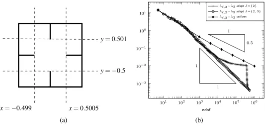
x=−0.499 x=0.5005

y=−0.5 y=0.501

(a)

10¹ 10² 10³ 10⁴ 10⁵ 10⁶ 10⁻³

10⁻² 10⁻¹ 10⁰ 10¹

1 1

1 0.5

ndof

λℓ,2−λ2adaptJ={2}

λℓ,2−λ2adaptJ={2,3}

λℓ,2−λ2uniform

(b)

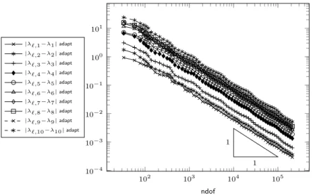
Figure 1.2.: Numerical test on a perturbed geometry. Uniform mesh-refinement (♦) leads to a sub- optimal convergence rate. Adaptive mesh-refinement which takes into account the residuals of only one discrete eigenfunction leads to the plateau in the convergence graph (+). Marking with respect to all discrete eigenfunctions in the cluster (o) leads to the optimal rate from the very beginning.

In practice, little perturbations in coefficients or in the geometry immediately lead to an eigenvalue cluster of finite length. Figure 1.2 displays an example with a narrow eigenvalue cluster where the algorithm of Dai et al. [2013] may fail in its original version. The small non-symmetry in the geometry generates an eigenvalue cluster of two simple eigenvalues

λ2=17.6557, λ3=17.6660.

The optimality results of Dai et al. [2008] and Carstensen and Gedicke [2012] for simple eigenvalues apply under the critical condition on the initial mesh to be sufficiently fine. A numerical computation with a coarse initial mesh (5 degrees of freedom) and conforming P1finite elements shows a large plateau up to 400 000 degrees of freedom in the convergence history (Figure 1.2b) of the eigenvalue error|λℓ,2−λ2|in the case that the adaptive mesh-refinement is driven by the error estimator contributions of the second discrete eigen- functionu_ℓ,2only. This numerical experiment reveals an unacceptable behaviour between 10 000 and 400 000 degrees of freedom for the algorithms of [Dai et al., 2008, Carstensen and Gedicke, 2012, Dai et al., 2013].

Adaptive mesh-refinement with respect to the error estimator contributions of both discrete eigenfunctionsu_ℓ,2andu_ℓ,3leads to the optimal convergence rate even for very coarse meshes. A heuristic explanation of this phenomenon will be given in Section 9.2. This pre- asymptotic failure of the known algorithms up to 400000 degrees of freedom motivates the study and design of adaptive FEMs for eigenvalue clusters. A first-glance generalisa- tion of the analysis of Dai et al. [2013] from multiple eigenvalues to clusters encounters the difficulty that the cluster width should not enter in the analysis as an additive term (cf.

Remark 4.13).

To illuminate the differences to the analysis of Dai et al. [2013], the first main aspect of this thesis is the analysis of the conforming P1 FEM computation of the eigenvalues of the Laplace operator. A cluster-robust reliability proof for the error estimator requires

(9)

(a) conformingP1 (b) nonconformingP1 (c) Morley (d) HCT Figure 1.3.: Mnemonic diagrams of some finite elements.

a new mathematical methodology (see Remark 4.13). The focus of the thesis, however, is on the a posteriori and optimality analysis of adaptive nonstandard finite elements for some eigenvalue problems in continuum mechanics, namely the Stokes and the biharmonic eigenvalue problem. The results are valid for the situation of eigenvalue clusters, but are also the first contributions for the case of simple eigenvalues.

One motivation for the use of nonconforming methods, especially for higher-order problems, is that they allow an easier implementation compared to conforming finite elements.

Figures 1.3c and 1.3d show the nonconforming Morley FEM in comparison to the conforming Hsieh-Clough-Tocher FEM based on a macro element. The computation of guaranteed lower eigenvalue bounds is a second motivation for nonconforming FEMs. The separation and resolution of the real eigenvalues requires known upper and lower eigenvalue bounds.

The min-max principle shows that upper eigenvalue bounds can be computed with any conforming FEM. Besides the easier practical implementation, nonconforming FEMs allow a convenient computation of lower eigenvalue bounds. This observation was first theoreti- cally justified by Armentano and Durán [2004] for singular eigenfunctions in an asymptotic regime. The recent works of Carstensen and Gedicke [2014], Carstensen and Gallistl [2014] and Liu and Oishi [2013] establish guaranteed lower eigenvalue bounds on arbi- trarily coarse meshes. For nonconforming methods, the constants of theL²error estimates for the related interpolation operators are known explicitly. The projection properties of those operators lead to the lower bounds of Carstensen and Gedicke [2014] and Carstensen and Gallistl [2014]. These results should be seen in comparison to the work of Liu and Oishi [2013] for the conformingP1FEM with anL²error estimate for the Galerkin projection. The involved constant depends on the mesh and has to be computed as an eigenvalue of a large-scale matrix. The advantage of nonconforming FEMs is that the interpolation functionals are well-defined for functions of minimal regularity and, therefore, the error estimates are valid element-wise. This thesis provides a unified framework for the aforementioned results and establishes lower bounds for the eigenvalues of the Stokes system as a new application,

Historical Overview

A basic overview of the finite element approximation of compact symmetric eigenvalue problems can be found in the textbook of Strang and Fix [1973]. A more abstract approach is summarised in the monograph of Chatelin [1983] and in the review articles of Babuška and Osborn [1991] and Boffi [2010]. An a priori error analysis for the nonconforming

(10)

FEM of eigenvalue problems dates back to Rannacher [1979]. The first a posteriori error estimates for eigenvalue problems were obtained by Verfürth [1994] within a general framework for nonlinear problems and by [Larson, 2000] by means of a duality technique while later Durán et al. [2003] employed techniques from the analysis of linear problems plus elementary algebra and higher-order convergence in theL²norm for the proof of a posteriori error bounds. Heuveline and Rannacher [2001] established a posteriori error bounds for nonsymmetric eigenvalue problems. The convergence of adaptive FEMs for eigenvalue problems was proven by Garau et al. [2009], Giani and Graham [2009] and Carstensen and Gedicke [2011]. An adaptive FEM based on the saturation assumption was proposed in [Carstensen et al., 2014d]. The proof of optimal convergence rates of AFEM for simple eigenvalues was given by Dai et al. [2008] and Carstensen and Gedicke [2012] for conforming FEMs and by Carstensen, Gallistl, and Schedensack [2014c] for a nonconforming FEM in the particular case of the first eigenvalue of the Laplacian. The first optimal convergence result of adaptive conforming finite element schemes with a multiple eigenvalue [Dai et al., 2013] suggests to use one bulk criterion for all discrete eigenfunctions in the algorithm for automatic mesh refinement.

Optimal convergence rates for the Stokes equations [Hu and Xu, 2013a] and the linear biharmonic problem [Hu et al., 2012] were recently established for the linear case. The recent work [Carstensen et al., 2014a] presents an axiomatic framework that unifies the optimality proofs that trace back to Stevenson [2007] and Cascon et al. [2008]. This approach also covers the optimality of the adaptive FEM computation of simple eigenvalues of the Laplacian of [Dai et al., 2008, Carstensen and Gedicke, 2012].

Ever since the pioneering work of Stevenson [2007], it has been understood that one key ingredient for the proof of optimal convergence rates of adaptive FEMs is the discrete reliability. For the nonconformingP1FEM on simply-connected domains in two space dimensions, the discrete reliability can be proven by means of the discrete Helmholtz decomposition of Arnold and Falk [1989]. Only very recently, discrete reliability for multiply- connected domains in any space dimensiond≥2 was proven by Carstensen, Gallistl, and Schedensack [2013a]. The main technical tool in the proof is a transfer operator between the non-nested finite element spaces. The design of an analogous operator for the Morley FEM appears more difficult because of the lack of a conforming subspace.

Main Results

One of the main aspects in the convergence analysis for eigenvalue problems is the error analysis of the eigenfunctions in theL²norm. The Aubin-Nitsche duality technique con- trols theL²error by the error in the energy norm times some power of the global mesh-size for conforming finite element methods. This methodology is not applicable to nonconforming FEMs because nonconforming functions are not admissible test functions in the continuous setting. This thesis enfolds conforming companion techniques to prove the L² control. For the nonconforming P1 FEM, the operator of Carstensen, Gallistl, and Schedensack [2014c] is generalised to any space dimension d ≥2. For the biharmonic eigenvalue problem and the Morley FEM from Figure 1.3c, a newC¹-conforming companion operator is developed based on the Hsieh-Clough-Tocher macro FEM [Ciarlet, 1978]

(see Figure 1.3d) and polynomial bubble functions of order 6. This enables the proof of an L²error estimate even for singular solutions withH^2+sregularity for 0<s≤1. The proofs

(11)

employ techniques from the medius analysis [Braess, 2009, Gudi, 2010, Carstensen et al., 2012b]. This means that, in contrast to classical a priori estimates, the results are true for any regularity of the eigenfunctions.

These results allow for the first optimality proofs for adaptive finite element computation of the Stokes and the biharmonic eigenvalue problems. The discrete reliability proof for the Morley FEM in this thesis is based on a novel discrete Helmholtz decomposition that generalises the recent decomposition of Carstensen, Gallistl, and Hu [2014b] to the case of simply supported and free boundary conditions.

In the adaptive scheme, the computable error estimator depends on the choice of the discrete eigenfunctions and is therefore not suitable for a convergence analysis based on a contraction property as in [Cascon et al., 2008, Stevenson, 2007]. This thesis follows the idea from [Dai et al., 2013] to employ a theoretical non-computable error estimator which allows a proof of equivalence to the refinement indicator of the adaptive algorithm. It turns out that the analysis of [Dai et al., 2013] is not directly applicable to the case of clustered eigenvalues. In contrast to the case of one multiple eigenvalue, care has to be taken that the reliability and equivalence estimates of the error estimator do not include the cluster width as an additive term. This thesis proves the first optimality result for adaptive finite element approximation of clustered eigenvalues with respect to the concept of nonlinear approximation classes.

One subtle aspect is the dependence of the parameters on the fineness of the initial mesh and the initial resolution of the cluster and its width. Therefore, the analysis in this thesis is explicit in all quantities that describe the eigenvalue cluster. To give an illustration of the dependence of the initial mesh-size, all constants in the optimality analysis for the conforming FEM for the Laplace eigenvalue problem are traced explicitly.

The optimality analysis is merely concerned with the approximation of the eigenfunctions. In order to obtain the optimal convergence rate for the eigenvalues, error estimates are needed that relate the eigenvalue error to the approximation error of the eigenfunctions within the cluster independent of the approximation error of all previous eigenfunctions.

Such a result for conforming discretisations was obtained by Knyazev and Osborn [2006].

Since this result makes use of the conformity by exploiting the min-max principle, their theorem cannot be directly applied to nonconforming finite elements. This thesis gives an extension of that result to nonconforming finite element spaces by applying the original result of Knyazev and Osborn [2006] to a modified setting where the spectrum with respect to the sum of the continuous and the finite element space is considered. The careful application of conforming companion operators enables certainL²and best-approximation results that eventually lead to the control of the eigenvalue error by the approximation error of the eigenvalue cluster.

Structure of the Thesis

Chapter 2 introduces the necessary notation and preliminaries on finite element meshes in R^dand their adaptive refinement and recalls some relevant inequalities. Chapter 3 outlines an abstract framework for the discretisation of eigenvalue clusters and provides an equivalence of error estimators. Section 3.3 presents an abstract approach to justify guaranteed lower eigenvalue bounds. The AFEM loop is introduced in Section 3.4. Chapter 4 proves optimal convergence rates of AFEM for the conformingP1discretisation of the eigenval-

(12)

ues of the Laplacian. Chapter 5 introduces the nonconformingP1FEM space and two nonstandard results, namely the existence of conforming companion operators and the discrete distance control [Carstensen, Gallistl, and Schedensack, 2013a]. The remaining parts of Chapter 5 prove optimality of the adaptive nonconforming FEM for the eigenvalues of the Laplacian. Chapter 6 presents a new application to the eigenvalues of the Stokes system.

Chapter 7 focuses on fourth-order eigenvalue problems and presents several new results on the nonconforming Morley finite element methods, namely an error estimate for the Morley interpolation operator, the existence ofC¹-conforming companion operators and a discrete Helmholtz decomposition. These results enable the proof of optimal convergence rates of the Morley FEM for the eigenvalues of the biharmonic operator. The optimality proofs in the Chapters 4, 5, 6, and 7 are based on the discrete reliability and the contraction property whose proofs can be found in the respective sections. Chapter 8 is devoted to error estimates which relate the eigenvalue error to the angle between the invariant subspaces in the case of nonconforming FEMs. Chapter 9 presents numerical tests for the model problems of this thesis on non-convex domains. It investigates the performance of the proposed algorithm for eigenvalue clusters in comparison to algorithms that rely on the multiplicity of the exact eigenvalues. Furthermore, the inclusion of an inexact linear-algebraic solve is investigated empirically. A table of basic notation is given in Appendix A. Appendix B gives an outline how to reproduce the numerical results with the software provided on an attached data medium (Appendix C).

Conclusions and Outlook

This thesis proves optimality of adaptive finite element methods for eigenvalue clusters of self-adjoint differential operators. The numerical experiments indicate that the require- ments on the initial mesh-size for the proposed algorithm are somehow weaker in comparison with algorithms that are based on the multiplicity of the exact eigenvalues.

In order to achieve optimal computational complexity, the AFEM loop has to be com- bined with an iterative eigenvalue solver and some termination criterion as proposed in [Miedlar, 2011]. The accuracy of the linear-algebraic solution is controlled by some param- eterκ. The optimality of algorithms of this type for sufficiently smallκ≪1 was analysed by Carstensen and Gedicke [2012] for conforming FEMs and by Carstensen, Gallistl, and Schedensack [2014c] for nonconforming FEMs. The results of this thesis is carried out for the caseκ=0, i.e., under the theoretical assumption that the discrete eigenvalue problems are solved exactly. The analysis can be extended to inexact solve with similar perturbation arguments as in [Carstensen and Gedicke, 2012, Carstensen, Gallistl, and Schedensack, 2014c]. The thesis proposes an adaptive algorithm which includes the iterative solve. This may be the first step towards optimal computational complexity for eigenvalue clusters.

The analysis of this thesis reveals that optimal convergence rates can be proven in the case of low-order finite elements whereas the treatment of higher-order methods remains an open problem, cf. Remark 4.21.

The analysis of non-selfadjoint eigenvalue problems encounters several additional dif- ficulties which cannot be covered with the analysis of this thesis. Recent developments on homotopy-based methods [Carstensen et al., 2011] are the objective of future research.

Nonlinear eigenvalue problems are a further challenge with high relevance in industrial

(13)

applications [Apel et al., 2002]. For most of these problems, the development of adaptive methods is still in its infancy and far from industrial practice.

Acknowledgement

The author thanks Professor C. Carstensen for the supervision of this thesis and Profes- sor V. Mehrmann for the collaboration in the project C22 “Adaptive solution of para- metric eigenvalue problems for partial differential equations ” within the DFG Research Center MATHEON. Moreover, the author thankfully acknowledges the support of the Deutsche Forschungsgemeinschaft (DFG), the support by the Chinesisch-Deutsches Zen- trum (project “The Adaptive Finite Element Method for the Fourth Order Problem”, grant no. GZ578), and by the Indian Department of Science and Technology (DST) (National programme on differential equations) which enabled the participation in several work- shops.

(14)

(15)

2. Preliminaries

This chapter clarifies the notation on function spaces (Section 2.1) and gives an overview of adaptive mesh-refinement in any space dimension (Section 2.2) and related data structures (Section 2.3). Section 2.4 reports some important results that will be frequently employed throughout the thesis.

The notation is summarised in the tables of Appendix A.

2.1. Function Spaces and Operators

LetΩ⊆R^d be a bounded open domain with polyhedral Lipschitz boundary. Throughout this thesis,d≥2 denotes the space dimension. The notationa≲bdenotes an inequality a≤Cb up to a multiplicative constant C that does not depend on the mesh-size or the eigenvalue cluster;a≈babbreviatesa≲b≲a.

Lebesgue and Sobolev Spaces

Standard notation on Lebesgue and Sobolev spaces [Adams and Fournier, 2003, Evans, 2010] applies throughout this thesis. Let (ω,F,µ) be a measure space and let (X,∥·∥) be a finite-dimensional real Banach space X ⊆R^M^×^N. For any µ-measurable function

f :ω →X, the Lebesgue integral is denoted by ´

ω f dµ and, if µ(ω)<∞, ffl

ω f dµ :=

µ(ω)⁻¹´

ω f dµ denotes the integral mean. TheL²seminorm is defined by

∥f∥L²(ω):=

ˆ

ω∥f∥²dµ1/2

.

Although neither the target setXnor the used measure may appear in this notation, they will be clear from the context. The space of equivalence classes of square integrable functions up to equality almost everywhere reads as

L²(ω;X):=

f :ω→X f is measurable and∥f∥L²(ω)<∞

∥·∥L²(ω)=0 andL²(ω):=L²(ω;R). The subset of L²(ω;X)-functions with vanishing integral is denoted byL²₀(ω;X)andL²₀(ω):=L²₀(ω;R). The space of (equivalence classes of) essen- tially bounded measurable functions is denoted byL^∞(ω)and the set ofX-valued functions whose components belong toL^∞(ω)is denoted byL^∞(ω;X). The essential supremum is denoted by∥·∥L^∞(ω)or∥·∥∞.

For a Lebesgue-measurable setω ⊆R^d and a Lebesgue-measurable function f :ω→ X with values in a finite-dimensional real Banach space X, the integral with respect to thed-dimensional Lebesgue measure is denoted by´

ω f dx. Thed-dimensional Lebesgue measure of ω is denoted by meas(ω). The integral over a (d−1)-dimensional hyper- surfaceΓwith respect to the(d−1)-dimensional Hausdorff measure reads as´

Γf dsand the(d−1)-dimensional Hausdorff measure ofΓis denoted by measd−1(Γ).

(16)

The set of infinitely differentiable functions from ω to X with compact support inω is denoted byD(ω;X)while D(ω):=D(ω;R). For any f ∈D(ω)and any multi-index α = (α1, . . . ,αd)∈N^d0of length|α|:=∑^d_j=1αj, the partial derivative with respect toα is defined via

D^αf:=∂^|α|f

∂x^α := ∂^|α|f

∂x^α¹···∂x^α^d.

For a bounded open Lipschitz domain ω ⊆R^d, a function f ∈L²(ω) is called k times weakly differentiable with respect toα, if there exists someg∈L²(ω)such that

ˆ

ω f D^αϕdx= (−1)^k ˆ

ωgϕdx for allϕ∈D(ω).

The function∂^|α|f/∂x^α:=D^αf:=gis calledk-th weak derivative with respect toα.

The Sobolev spaceH^k(ω)is defined by H^k(ω):=

f ∈L²(ω)for allα∈N^d0 with|α| ≤kthere existsD^αf∈L²(ω) . The set ofX-valued functions whose components belong toH^k(ω)is denoted byH^k(ω;X).

The finite-dimensional Banach spaceX⊆R^M^×^N may be identified withR^mfor somem∈ N. Define for any f= (f₁, . . . ,fm)∈H^k(ω;X)the norm

∥f∥H^k(ω):=



|α|≤

∑

k m

∑

j=1∥D^αfj∥²L²(ω)

1/2

.

The closure of D(ω;X) with respect to the norm ∥·∥H^k(ω) is denoted by H₀^k(ω;X) and H₀^k(ω):=H₀^k(ω;R).

Fork∈Nand 0<s≤1 define the Sobolev space H^k+s(ω):=

v∈L²(ω)∥v∥H^k+s(ω)<∞ for the Sobolev–Slobodeckij norm

∥v∥H^k+s(ω):=



∥v∥²H^k(ω)+

∑

|α|=k

ˆ

ω

ˆ

ω

|D^αv(ξ)−D^αv(η)|²

|ξ−η|^d+2s dx(ξ)dx(η)

1/2

.

Differential Operators

Definition 2.1(derivative, divergence). For a sufficiently smooth function f:Ω→R^m, the first (weak) derivative is denoted byD f and the second derivative is denoted byD²f. For a sufficiently smooth vector fieldβ:Ω→R^d, the divergence reads as divβ:=∑^d_j=1∂βj/∂xj. For a sufficiently smooth tensor fieldσ :Ω→R^d^×^d, the divergence is applied row-wise, i.e., divσ:= (divσ1•;. . .;divσd•). The Laplacian reads as∆:=divD^⊤and the biharmonic operator (also called the bi-Laplacian operator) is defined as∆²:=∆∆. ♦ Remark 2.2. If f :Ω→R^m form≥1, then D f always denotes the JacobianD f :Ω→

R^m^×^d. ♦

(17)

2.2. Adaptive Finite Element Meshes in Any Space Dimension Definition 2.3(Curl operator). Letd =2 and define for any smooth function f :Ω→R its Curl as

Curlf:= (−∂f/∂x₂ ∂f/∂x₁).

For a sufficiently smooth vector fieldβ :Ω→R², define Curlβ :=

−∂β1/∂x₂ ∂β1/∂x₁

−∂β2/∂x₂ ∂β2/∂x₁



. ♦

2.2. Adaptive Finite Element Meshes in Any Space Dimension

This section describes the data structures and refinement rules for adaptive mesh-generation in d space dimensions. This refinement algorithm traces back to Maubach [1995] and Traxler [1997]. The presentation in this section follows the description of Stevenson [2008]

and recalls some results from Carstensen, Gallistl, and Schedensack [2013a].

Regular Triangulations

Definition 2.4(tagged simplex). A tagged simplex(z₀, . . . ,zd;γ)is a (d+2)-tuple with vertices(z₀, . . . ,z_d)∈

R^dd+1

, which do not lie on a(d−1)-dimensional hyperplane, and

a typeγ∈ {0, . . . ,d−1}. ♦

The mapping

dom :

R^dd+1

× {0, . . . ,d−1} →2^R^d

extracts the corresponding (closed) simplex dom(z0, . . . ,zd;γ):=conv{z₀, . . . ,zd} from a tagged simplex(z0, . . . ,zd;γ).

If there is no risk of confusion, a tagged simplex is identified with its domain. Given tagged simplices T,T^′, define for abbreviation ∂T :=∂dom(T), T∩T^′ :=dom(T)∩ dom(T^′),T∪T^′:=dom(T)∪dom(T^′),v|^T :=v|dom(T), int(T):=int(dom(T)). Let fur- thermorez∈T abbreviatez∈dom(T).

Definition 2.5(regular triangulation). A finite setTof tagged simplices is called regular triangulation of Ω, if it covers the domain in the sense that Ω=^_T_∈Tdom(T) and any two distinct simplices(T₁,T₂)∈T²withT₁= (z₀, . . . ,z_d;γ1)andT₂= (y₀, . . . ,yd;γ2)with T₁̸=T₂are either disjoint or share exactly one lower-dimensional surface in the sense that there existn∈ {1, . . . ,d}and(j₁, . . . ,jn)∈ {0, . . . ,d}ⁿand(k1, . . . ,kn)∈ {0, . . . ,d}ⁿsuch that

T₁∩T₂=conv{zj₁, . . . ,zj_n}=conv{yk₁, . . . ,yk_n}. ♦ Definition 2.6(vertices and hyper-faces). Given a tagged simplexT = (z₀, . . . ,z_d;γ), its set of vertices is denoted by

N(T):={z₀, . . . ,z_d}. The set of hyper-faces reads as

F(T):= conv

N(T)\ {zk} k∈ {0, . . . ,d}

. ♦

(18)

@

@@

@

@@ @

@@

@@ @

@@

@

@@

Figure 2.1.: Possible refinements of a triangleT in one level in 2D. The thick lines indicate the refinement edges of the sub-triangles.

Bisection

Definition 2.7(bisection of a simplex). LetT = (z₀, . . . ,z_d;γ)be a tagged simplex. The two tagged simplices

z₀,z₀+zd

2 ,z₁, . . . ,z_γ,z_γ+1, . . . ,z_d₋₁;(γ+1)modd

and

zd,z₀+zd

2 ,z₁, . . . ,z_γ,zd−1, . . . ,z_γ+1;(γ+1)modd (2.1) are called the children of T. (By convention, the finite sequence (z_γ+1, . . . ,zd−1) and (z1, . . . ,z_γ) is void for γ =d−1 and γ =0, respectively.) Any child of some child of T is called grandchild; conversely, T is called a parent (resp. grandparent) of each of its two children (resp. four grandchildren). A simplex generated fromT by a finite number of

applications of (2.1) is called a descendant ofT. ♦

The following proposition ensures that grandchildren do not share hyper-faces with their grandparents.

Proposition 2.8. Any grandchild T of a tagged simplex K satisfiesF(T)∩F(K) = /0. Proof. This follows from the definition of the bisection rule (2.1). A detailed proof is given in [Carstensen, Gallistl, and Schedensack, 2013a, Proposition 2.1].

Initial Conditions

The initial condition from [Stevenson, 2008, p. 232] described in Definition 2.10 below guarantees that successive refinements of a regular triangulationTlead to regular triangulations. The notion of a reflected neighbour [Stevenson, 2008] is required for the statement of that initial condition. Note that, given a tagged simplexT = (z0, . . . ,zd;γ), the simplex

TR:= (zd,z1, . . . ,z_γ,zd−1,z_d₋₂, . . . ,z_γ+1,z0;γ) with dom(TR) =dom(T)has the same children asT.

Definition 2.9 (neighbour, reflected neighbour). Two tagged simplices T, K are called neighbours, if they share a common(d−1)-dimensional surface (i.e., a hyper-face in the sense of Definition 2.6). Two neighbouring tagged simplicesT andK are called reflected neighbours, if the ordered sequence of vertices of eitherT orTR coincides with that ofK

on all but one position. ♦

The following initial condition from [Stevenson, 2008] is crucial for the regularity of refinements.

(19)

2.2. Adaptive Finite Element Meshes in Any Space Dimension Definition 2.10 (initial condition). A regular triangulation Tis said to satisfy the initial condition, if all simplices inT are of the same typeγ and any two neighbouring tagged simplicesT = (y₀, . . . ,y_d;γ)andK= (z₀, . . . ,z_d;γ)satisfy

(a) If conv{y₀,yd} ⊆T∩Kor conv{z₀,zd} ⊆T∩K, thenT andKare reflected neighbours.

(b) If conv{y₀,y_d} ̸⊆T∩K̸=/0 and conv{z₀,zd} ̸⊆T∩K, then any two neighbouring

children ofT andKare reflected neighbours. ♦

This condition guarantees that uniform refinements of a triangulation T are regular [Stevenson, 2008, Theorem 4.3] which transfers to the refinement routine of the following subsection.

Admissible Triangulations

Throughout this thesis, the initial regular triangulationT0 ofΩis assumed to satisfy the initial condition from Definition 2.10. A regular triangulation Tis called an admissible refinement of T0 if it is a regular triangulation and it was created by refining T0 with a successive application of the bisection rule (2.1).

The set of all admissible triangulations is denoted byT. This set is known to be uniformly shape-regular [Stevenson, 2008] in the sense that the ratio of the diameter and the radius of the largest inscribed ball is uniformly bounded only dependent onT0. For any T∈T,

T(T):={T^′∈T|T^′is an admissible refinement ofT}.

Let, for anym∈N, the set of triangulations inTwhose cardinality differs from that ofT0

bymor less be denoted by

T(m):={T∈T|card(T)−card(T0)≤m}.

Definition 2.11(overlay). Given two admissible triangulations (T,K)∈T², the overlay T⊗Kis defined as the smallest common refinement ofTandKin the sense thatT⊗K∈T satisfies

T(T)∩T(K) =T(T⊗K). ♦ Lemma 2.12. Any(T,K)∈T²satisfy

card(T⊗K)−card(T)≤card(K)−card(T0). (2.2) Proof. See Lemma 3.7 of [Cascon et al., 2008].

Notice thatT1∈T(T2) andT2∈T(T1) implies T1=T2. For any T ∈T, the routine refine(T,T)from [Stevenson, 2008, p. 235] computes a refinementT∈T(T)such that T ∈T\T. It is repeated here for convenient reading. For a simplexT =conv{z₀, . . . ,z_d}, the edge conv{z₀,zd}is called its refinement edge.

Algorithm 2.13(refine(T,T)).

Input: T∈TandT ∈T setK:=/0,R:={T} whileR̸=/0do

(20)

Rnew:=/0 forT^′∈Rdo

forT^′′∈Tthat are neighbours ofT^′withT^′′∈/R∪Kdo ifT^′′andT^′have the same refinement edgethen

Rnew:=Rnew∪ {T^′′} else

T:=refine(T,T^′′)

add toRnewthe child ofT^′′that is a neighbour ofT^′ end if

end for end for

K:=K∪RandR:=Rnew end while

forT^′∈Kdo

bisectT^′ into childrenT₁^′,T₂^′ and updateT:= (T\ {T^′})∪ {T₁^′,T₂^′} end for

Output: T ♦

The following proposition proven in [Stevenson, 2008, Theorem 5.1] assures the minimality of this routine. In case thatT̸∈Tsetrefine(T,T):=T.

Proposition 2.14. The outputT:=refine(T,T)is a regular triangulationT∈Tand is minimal in the sense that any other refinement T∈T(T) with T ∈T\T is a refinement T∈T(T)ofT.

For a set of simplicesM⊆T, the routinerefine(T,M)runs the following loop.

Algorithm 2.15(refine(T,M)).

Input: T∈TandM⊆T SetT:=T

whileM∩T̸=/0do chooseT∈M∩T

computeT:=refine(T,T) end while

Output: T ♦

This loop computes a refinementT∈T(T)ofT by applyingrefine(T,T)for simplices inMand results in a triangulation in which all simplices ofM⊆T\T are refined. The following proposition guarantees that the result is independent of the order ofT ∈M∩T in the loop of refineand furthermore states the minimality ofrefinefor any input set M⊆T.

Proposition 2.16. The output T:=refine(T,M) does not depend on the selection of T ∈M∩Tin Algorithm 2.15. The outputT:=refine(T,M)is minimal in the sense that any other refinementT^′∈T(T)withM⊆T\T^′is a refinementT^′∈T(T).

Proof. See Propositions 2.2 and 2.4 of [Carstensen, Gallistl, and Schedensack, 2013a].

The following fundamental result proven by Binev et al. [2004] ford=2 and by Steven- son [2008] ford≥2, is one of the main tools for the proof of optimal convergence rates.

(21)

2.2. Adaptive Finite Element Meshes in Any Space Dimension Theorem 2.17(Binev et al. [2004], Stevenson [2008]). Let(Tj | j∈N⁰)∈T^N⁰ be a sequence of regular triangulations and let(Mj |j∈N⁰)be a sequence of subsetsMj⊆Tj

(for all j∈N0) such that

Tj+1=refine(Tj,Mj) for all j∈N⁰.

Then there exists a constant C_BDVsolely dependent onT0such that, for anyℓ∈N, it holds that

card(Tℓ)−card(T0)≤C_BDV

ℓ−1 j=0

∑

card(Mj).

One-Level Refinements

The remaining parts of this section present a result of a private communication with Steven- son [2013].

Definition 2.18(level). LetT∈Tbe a an admissible triangulation refined from T0. For anyT ∈Tthere exists an ancestorK∈T0withT ⊆K. The level ofT, is defined by

ℓ(T):=meas(T)

meas(K).

In other words,ℓ(T)is the number of applications of the bisection rule (2.1) that are needed

to obtainT fromK. ♦

Lemma 2.19. Let T ∈TandT^′:=refine(T,T). If T^′∈T^′is newly created by this call ofrefine(T,T), i.e., T^′∈T^′\T, then

(a) ℓ(T^′)≤ℓ(T) +1, (b) dist(T^′,T)≲2⁻^ℓ(T^′^)/d. Moreover,

(c) there exists a constant C >0 such that, for all T∈T and any (T,K) ∈T² with T∩K̸=/0, it holds that|ℓ(T)−ℓ(K)| ≤C;

(d) there exists a constant c >0 such that, for all T∈T and any (T,K)∈T² with ℓ(T)> ℓ(K) +C, it holds thatdist(K,T)≥c2⁻^ℓ(K)/d.

Proof. The first two assertions follow from [Stevenson, 2008, Thms. 5.1–5.2]. Properties (c)–(d) follow from the shape-regularity.

The following proposition implies that the number of refinements of anyK∈Tgenerated by a call ofrefine(T,T)is uniformly bounded.

Proposition 2.20. Let T ∈TandT^′=refine(T,T). Let K∈Tand K^′∈T^′ with K^′⊆K be its descendant in the sense of Definition 2.7. Then it holds that

ℓ(K^′)−ℓ(K)≲1.

(22)

Proof. Ifℓ(K^′) =ℓ(K), the assertion is trivially satisfied. Hence, assumeℓ(K) +1≤ℓ(K^′). By (a) from Lemma 2.19,ℓ(K^′)≤ℓ(T) +1 and soℓ(K)≤ℓ(T). Recall the constantCfrom Lemma 2.19.

Case 1. Ifℓ(T)≤ℓ(K) +C, then (a) from Lemma 2.19 implies thatℓ(K^′)≤ℓ(T) +1 and, hence,ℓ(K^′)≤ℓ(K) +C+1.

Case 2. Ifℓ(T)> ℓ(K) +C, then (d) implies that dist(T,K)≳2^−ℓ(K)/d, whence dist(T,K^′)≳2⁻^ℓ(K)/d.

On the other hand, (b) states that

dist(K^′,T)≲2⁻^ℓ(K^′^)/d. The foregoing two inequalities imply

2^−ℓ(K)/d≲2^−ℓ(K^′^)/d and soℓ(K^′)−ℓ(K)≲1.

The following proposition generalises Proposition 2.20 to the case of a marked setM⊆ T.

Proposition 2.21. Let T^′ ∈T(T) be some one-level refinement of T, i.e., there exists a subsetM⊆TwithT^′=refine(T,M), and let K∈T, K^′∈T^′ with K^′⊆K, i.e., K^′ is a descendant of K. Then, there exists a constant C>0with

ℓ(K^′)−ℓ(K)≤C.

Proof. It holds that

T^′= ^

T∈M

refine(T,T),

i.e.,T^′is the overlay of allrefine(T,T)withT ∈M. The concept of binary trees [Binev et al., 2004] shows that there exists T ∈M with K^′ ∈refine(M,T). Thus, Proposi- tion 2.20 proves the assertion.

2.3. Data Structures

Definition 2.22(piecewise polynomials). LetTℓ∈T. For any subsetω⊆Ω, the space of polynomial functions of total degree≤kis denoted byPk(ω). LetX ⊆R^M^×^N be a finite- dimensional Banach space. TheX-valued functions whose components belong toPk(ω) are denoted by Pk(ω;X). For a regular triangulation Tℓ of Ω, the spaces of piecewise polynomials read as

Pk(Tℓ):=

v∈L^∞(Ω)∀T ∈Tℓ,v|^T∈Pk(T) , Pk(Tℓ;X):=

v∈L^∞(Ω;X)∀T∈Tℓ,v|^T ∈Pk(T;X) .

The L²-orthogonal projection onto the space Pk(Tℓ) (or Pk(Tℓ;X)) is denoted by Π^k_ℓ or Π^k_T

ℓ. ♦

(23)

2.4. Frequently Used Results Definition 2.23(midpoints). The centre of gravity of a simplexT (resp. a hyper-faceF) is

denoted by mid(T)(resp. mid(F)). ♦

Definition 2.24(notation of vertices and hyper-faces). Letω ⊆ΩandΓ⊆∂Ω. Define Nℓ:=N(Tℓ):=∪^T∈TℓN(T)as the set of vertices ofTℓ. The set of vertices that belong to ω is denoted byNℓ(ω):=Nℓ∩ω. The hyper-faces ofTℓ are denoted byFℓ:=F(Tℓ):=

∪T∈TℓF(T). The hyper-faces that lie insideΩread asFℓ(Ω):={F∈Fℓ|F̸⊆∂Ω}and the hyper-faces that belong toΓread asFℓ(Γ):={F∈Fℓ|measd−1(F∩Γ)>0}. Furthermore,

defineFℓ(Ω∪Γ):=Fℓ(Ω)∪Fℓ(Γ). ♦

Definition 2.25(patches). Letz∈Nℓ,F∈FℓandT ∈Tℓ. The set of simplices that share z reads as Tℓ(z):={K∈Tℓ|z∈K}. The set of simplices that share F is defined as Tℓ(F):={K∈Tℓ|F∈F(K)}. The patchesωz,ωF andωT read as

ωz:=int(∪Tℓ(z)), ωF :=int(∪Tℓ(F)),

ωT :=int(∪{K∈Tℓ|T∩K̸= /0}). ♦ Definition 2.26(mesh-size). ForT∈Tℓdefineh_T:=meas(T)^1/d. ForF∈Fℓdefineh_F :=

diam(F). The piecewise constant functionh_ℓ:=h_T_ℓ∈P0(Tℓ)is defined byh_T_ℓ|^T:=h_T for

eachT ∈Tℓ. ♦

Definition 2.27(normals and jumps). AnyF∈F(Tℓ)is associated to a fixed orientation of the unit normalνF onF; on the boundary,νF is the outer unit normal ofΩ. For an interior hyper-faceF̸⊆∂Ωthe orientation is fixed through the choice of the simplicesT₊∈Tℓand T₋∈TℓwithF=T₊∩T₋andνF =νT₊|^F (i.e.νFpoints outwards ofT₊). In this situation, [v]_F :=v|^T+−v|^T₋ denotes the jump acrossF. For a hyper-faceF⊆∂Ωon the boundary,

the jump across this hyper-surfaceFis[v]_F:=v. ♦

Definition 2.28(piecewise action of differential operators). LetTℓbe a regular triangulation. The piecewise action of a differential operator is indicated by the subscript NC, i.e., the piecewise versions ofD,D², div,∆,∆², Curl read asD_NC,D²_NC, divNC,∆_NC,∆²_NC, CurlNC,

e.g.,(D_NCv)|^T =D(v|^T)for anyT ∈Tℓ. ♦

Definition 2.29(oscillations). Let(p,k)∈N²0andf∈L²(Ω;X). For a regular triangulation TℓofΩthe oscillations are defined as

osc²_p,k(f,Tℓ):=∥h^k_ℓ(1−Π^p_ℓ)f∥²L²(Ω) and oscp,k(f,Tℓ):=

osc²_p,k(f,Tℓ). ♦

2.4. Frequently Used Results

This section reports some important estimates and identities that are used throughout the analysis of this thesis.

Proposition 2.30(Young inequality). Any(a,b,ε)∈R³withε>0satisfy 2ab≤εa²+ε⁻¹b².

Proof. The formula 0≤(ε^1/2a−ε⁻^1/2b)²=εa²+ε⁻¹b²−2abproves the result.

(24)

Proposition 2.31(trace identity, trace inequality). Let T be a simplex with F∈F(T)and PF ∈N(T)\ {F}the vertex opposite to F∈F(T). Then any v∈H¹(int(T))satisfies the trace identity

F

v ds=

T

v dx+1

d _TDv(• −PF)dx as well as the trace inequality

∥v∥²L²(F)≲h⁻_T¹∥v∥²L²(T)+hT∥Dv∥²L²(T).

Proof. The proof of the trace identity follows from the integration by parts formula, see [Carstensen and Funken, 2000]. The trace inequality is a consequence of that identity and the Young inequality. For a proof see, e.g., [Di Pietro and Ern, 2012].

Proposition 2.32(discrete Friedrichs inequality). LetTℓbe a regular triangulation ofΩ.

Any piecewise smooth v∈L²(Ω), in the sense that v|int(T)∈H¹(int(T))for any T ∈Tℓ, with´

∂Ωv ds=0satisfies

∥v∥L²(Ω)≲



∑

F∈Fℓ(Ω)

h^d_F⁻²ffl

F[v]Fds21/2

+∥D_NCv∥L²(Ω)

where the constant hidden in the notation≲only depends onΩand the shape-regularity ofTℓ. IfΩis a simplex, any piecewise smooth v∈L²(Ω)satisfies

∥v∥L²(Ω)≲diam(Ω)⁽²⁻^d)/2



 ˆ

∂Ωv ds



 +diam(Ω)



∑

F∈Fℓ(Ω)

h^d_F⁻²ffl

F[v]Fds21/2

+∥D_NCv∥L²(Ω)



where the constant hidden in the notation≲only depends on the shape-regularity ofTℓ. Proof. The proof can be found in [Brenner and Scott, 2008, Thm. 10.6.12] or [Brenner, 2003]. The dependence on diam(Ω) in the second inequality can be obtained by tracing the dependence of diam(Ω)in the proof of [Brenner and Scott, 2008, Thm. 10.6.12] for the volume term and by a scaling argument for the boundary term.

The following proposition is a consequence of a result of Kato [1966, Thm. 6.34 in Chapter 1, §6].

Proposition 2.33 (Kato [1966]). Let (H,⟨·,·⟩^H) be a Hilbert space with induced norm

∥·∥^Hand let X ⊆H, Y⊆H be finite-dimensional subspaces withdimX =dimY <∞. Let PX and PY denote the orthogonal projections onto X and Y , respectively. Then it holds that

∥PX−PY∥^H≤ ∥(1−PX)PY∥^H=∥(1−PY)PX∥^H where∥·∥^H abbreviates the operator norm∥·∥L(H,H).

(25)

2.4. Frequently Used Results

Proof. Theorem 6.34 of [Kato, 1966, Chapter 1, §6, p. 56] states that the condition δ1:=∥(1−P_Y)PX∥^H<1

and dimX=dimY <∞imply thatPY|^X :X →Y is an isomorphism and

∥P_X−P_Y∥^H=∥(1−P_X)PY∥^H=∥(1−P_Y)PX∥^H.

(Here, the finite dimension ofX andY is required to see that an injective mapping is an isomorphism.) By symmetry this is also true in case that δ2:=∥(1−P_X)PY∥H <1. In the remaining case that min{δ1,δ2} ≥1, the fact thatP_X andP_Y are orthogonal projections leads toδ1=δ2=1. In this case, the stated inequality is proven following the arguments of [Kato, 1966]. For anyw∈H, the Pythagoras theorem shows

∥(PX−PY)w∥²H=∥(1−PY)PXw−PY(1−PX)w∥²H=∥(1−PY)PXw∥²H+∥PY(1−PX)w∥²H. Hence, the fact that the projections P_X and(1−P_X) are idempotent and the Cauchy inequality imply

∥(PX−PY)w∥²H≤ ∥(1−PY)PX∥²H∥PXw∥²H+∥PY(1−PX)∥²H∥(1−PX)w∥²H.

A direct calculation reveals that ∥PY(1−PX)∥^H =∥(1−PX)PY∥^H =δ2=1. This and

∥(1−PY)PX∥^H=δ1=1 imply with the Pythagoras theorem that

∥(PX−P_Y)w∥²H≤ ∥P_Xw∥²H+∥(1−P_X)w∥²H=∥w∥²H. This concludes the proof.

Corollary 2.34. Let(H,⟨·,·⟩^H)be a Hilbert space with induced norm∥·∥^Hand let X⊆H, Y ⊆H, Z⊆H be finite-dimensional subspaces withdimX=dimY =dimZ<∞. Then it holds that

sup

x∈X

∥x∥H=1

yinf∈Y∥x−y∥H= sup

y∈Y

∥y∥H=1

xinf∈X∥y−x∥H and sup

x∈X

∥x∥H=1

yinf∈Y∥x−y∥^H≤ sup

x∈X

∥x∥H=1

zinf∈Z∥x−z∥^H+ sup

z∈Z

∥z∥H=1

yinf∈Y∥z−y∥^H.

Proof. LetPX,PY andPZ denote the orthogonal projection ontoX,Y andZ, respectively.

The stated identity directly follows from Proposition 2.33 sup

x∈X

∥x∥H=1

yinf∈Y∥x−y∥^H=∥(1−PY)PX∥^H=∥(1−PX)PY∥^H= sup

y∈Y

∥y∥H=1

xinf∈X∥y−x∥^H.

Similarly, the stated inequality follows from the triangle inequality

∥(1−PY)PX∥^H≤ ∥(1−PY)PZ∥^H+∥(1−PY)(PZ−PX)∥^H≤ ∥(1−PY)PZ∥^H+∥PZ−PX∥^H and the inequality of Proposition 2.33.

(26)

Remark 2.35 (angles). One can reformulate the results of Proposition 2.33 and Corol- lary 2.34 in terms of the largest principal angle between subspaces with

sin²∠(X,Y) =∥(1−PY)PX∥²H= sup

x∈X

∥x∥H=1

yinf∈Y∥x−y∥²H.

Indeed, for anyx∈ X\ {0}with orthogonal projectiony:=P_Yx̸=0 ontoY, the definition of the angle and|⟨x,y⟩^H|=∥PYx∥^H∥y∥^Hlead to

sin²∠(x,y) =1− ⟨x,y⟩²H

∥x∥²H∥y∥²H

=1−∥PYx∥²H

∥x∥²H

=∥x−PYx∥²H

∥x∥²H

=sin²∠(span{x},Y).