Chapter 1 Finite Element Methods

Chapter 1

Finite Element Methods

In this chapter we will consider how one can model the deformation of solid objects un- der the influence of external (and possibly internal) forces. As we shall see, the coupled equations can be cast into a matrix equation, which can be solved using e.g. the LU- decomposition method.

Literature:

1. Carlos A. Felippa, “Introduction to Finite Element Methods”, http://www.colorado.edu/engineering/CAS/courses.d/IFEM.d/

1.1 Behavior of solids: strain and stress

1.1.1 Modeling a solid using displacement vectors

Let us find a method for modeling a solid block of material with size L

× L

× L

. We assume that at rest the block of solid does not have any internal stresses. Let us define a cartesian coordinate system (X, Y, Z). We can now give a label to each point in the block with the coordinates at which that point is. We use lower-case letters for that: (x, y, z).

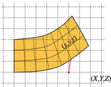
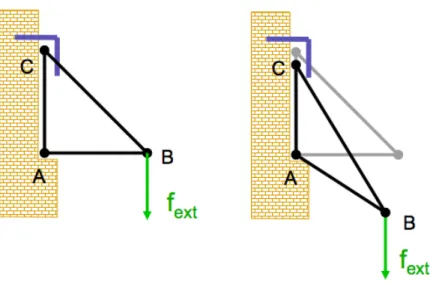
The reason why we use lower case letters for labeling the points in the solid, while using upper case letters for the spatial coordinates is because only in the relaxed case the two are the same, while in the case of deformation, displacement or rotation, the two are different (see Fig.1.1).

In general, we can assign a spatial location (X, Y, Z ) to each element of the block (x, y, z). So initially, in the relaxed state, we have

X(x, y, z) = x (1.1)

Y (x, y, z) = y (1.2)

Z(x, y, z) = z (1.3)

But if we translate the block by a vector (∆x, ∆y, ∆z), then we obtain:

X(x, y, z) = x + ∆x (1.4)

Y (x, y, z) = y + ∆y (1.5)

Z(x, y, z) = z + ∆z (1.6)

Figure 1.1: A picogram showing how the internal material coordinates (x, y, z) and the spatial coordinates (X, Y, Z) relate to each other in case of a material deformation.

Rotation of the block around the z-axis by an angle θ would give

X(x, y, z) = x cos θ − y sin θ (1.7)

Y (x, y, z) = x sin θ + y cos θ (1.8)

Z(x, y, z) = z (1.9)

Both translation and rotation do not induce any stresses in the block. For that, you need to deform the block. For instance, a bending of the block in y-direction could look like

X(x, y, z) = x (1.10)

Y (x, y, z) = y + ax

(1.11)

Z (x, y, z) = z (1.12)

where a gives the degree of bending.

For mathematical convenience we introduce the displacement vector field

δ

(x, y, z) = X(x, y, z) − x (1.13)

δ

(x, y, z) = Y (x, y, z) − y (1.14)

δ

(x, y, z) = Z(x, y, z) − z (1.15)

It is with these displacement vectors that we will do our calculations from now on.

1.1.2 Deformation of solids: strain

A non-zero displacement does not necessarily mean that the object is deformed. At every position (x, y, z) in the object we can calculate the strain tensor

ε

= 1

2 (∂

δ

+ ∂

δ

) (1.16)

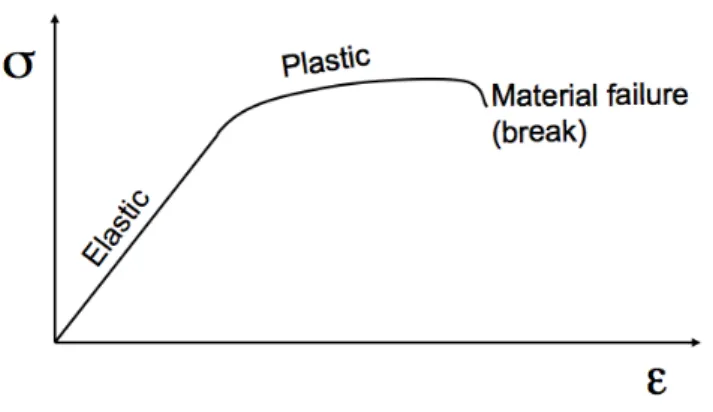
Figure 1.2: Stress response regimes of a solid material to an imposed strain.

The strain tensor tells how deformed the object it. A zero strain tensor means that there is no deformation in the material at that position. Note that the strain does not yet tell anything about the internal forces in the material. As we shall see below, strain induces stresses, but which stresses it induces depends on material properties.

Let us give an example in 2-D:

ε =

∂

X − 1

(∂

Y + ∂

X)

1

2

(∂

Y + ∂

X) ∂

Y − 1

(1.17) In the above example of the strain tensor the diagonal elements give the stretching or compression deformation. The off-diagonal elements give the shear strain.

1.1.3 Material reaction to strain: stress

Due to the internal structure of solids, a strain imposed on a solid body will induce internal stresses. A stress is like a force per unit surface. We will denote the stress as a tensor σ

. The components of σ

and ε

are related to each other in a linear way (as we will discuss below). However, this linear relation only holds for strains that are small enough. As an example consider a block of granite: it is extremely strong (inducing very large σ

for very modest ε

), but if stretched to more than a percent or so, it will break. Most materials have a linear response to small strains (the so-called “elastic” regime), then beyond a certain strain threshold the respons weakens (the so-called “plastic” regime), and then beyond an even larger strain threshold the material will break (see Fig. 1.2).

1.1.4 Stress-strain relation for isotropically elastic material

For simple elastic materials with no internal preferential directions and isotropic response, Hooke’s law holds for small enough strains:

ε

= 1

E σ

(1.18)

where E is called Young’s modulus. In reaction to a stretch in e.g. 1-direction (i.e. x-

direction) the material counters with a force that tries to counteract this stretch. One

can also invert this statement: when a given force per unit surface σ

acts in x-direction

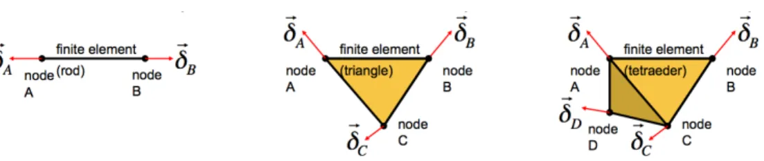
Figure 1.3: The most basic finite elements: 1-D rod, 2-D triangle and 3-D tetraeder.

on a block of material, then in response the block will deform according to ε

= σ

/E.

Typically a material will also deform in the perpendicular directions:

ε

= ε

= − νε

= − ν

E σ

(1.19)

When we stretch a material in x-direction, it will typically get thinner in y and z direction.

The parameter ν is the Poisson ratio. If it is 0.5, the material is incompressible, i.e. it maintains a constant density. If it is negative, the material expands in y and z direction when it is stretched in x-direction. There are materials that have this pecular behavior, but it is rare. For most materials it is between 0 and 0.5. For all materials it is between -1 and 0.5. A few examples: most metals have ν ∼ 0.3 · · · 0.4, concrete has ν ≃ 0.2 and cork has ν ≃ 0.

In general one can thus write:



 ε

ε

ε



 = 1 E





1 − ν − ν

− ν 1 − ν

− ν − ν 1







 σ

σ

σ



 (1.20)

In addition to the parallel and transverse stresses and strains, one also has shear. This is given by the non-diagonal elements of the tensors: The shear strain components are ε

, ε

and ε

while the shear stress components are σ

, σ

and σ

. However, we will ignore these in this lecture.

1.2 Finite Element Methods (FEM) for solids

The equations and methods described in Section 1.1 showed the basic principles of how solids are modeled. But the method for solving the motion and deformation of solid objects in that section is not often used, because it can not naturally treat complex structures. In practice engineers want to be able to solve for the motion or the static structure of complex objects such as bridges, houses, ships, cars, airplanes etc. What they then often use is a

“Finite Element Method” (FEM). With this method the object can be constructed out of individual blocks of varying shapes, glued together to form a full object. See Fig.1.3 for the most basic 1-D, 2-D and 3-D finite elements. This does not mean that it would not be possible to introduce more complex finite elements. On the contrary: one can certainly also include squares, cubes etc. But the advantage of rods, triangles and tetraeders is that in those simple finite elements the stress tensor is constant throughout the element (at least in the linear regime).

To keep things simple, we will use (instead of triangles, tetraeders, cubes etc) just

simple 1-D rods. It turns out that you can already produce relatively complex 2-D and

3-D structures, just by connecting rods together. We will use the direct stiffness method (DSM) to solve for the deformation of the shape of a solid object built out of a set of rods (=1D finite elements).

1.2.1 DSM: A 1-D finite element in 1-D

Let us consider a 1-D rod in 1-D space. The rod has length L, radius r and Young’s modulus E. We model the rod by first defining two nodes: Node A having X

= 0 and node B having X

= L (the superscript (0) means: before the deformation). We now stretch (or squeeze) this rod in the x-direction (the only direction we have, for now). So we impose a displacement of node A, which we denote by δx

and a displacement of node B, which we denote by δx

. So we have

X

= X

+ δx

(1.21)

X

= X

+ δx

(1.22)

We can now ask ourselves: Which external force f

do we have to impose on node A and external force f

do we have to impose on node B such that we can achieve the displacements δx

and δx

? To answer this equation, let us consider first the case δx

= 0 and vary δx

. If δx

< 0, i.e. if we stretch the rod by pulling on A while keeping B fixed, then this can only be done if we indeed impose a force f

= Kδx

on node A, where the stiffness coefficient K is given by

K = Eπr

/L (1.23)

But we have to impose the opposite force on node B, otherwise the rod would experience a netto force and start accelerating and fly away. So we have f

= − Kδx

. A similar logic can be used for the case when we keep δx

= 0 and put δx

6 = 0. All of this can be expressed in matrix form:

f

f

=

K

K

K

K

δx

δx

= K

1 − 1

− 1 1

δx

δx

(1.24) The matrix is called the stiffness matrix.

So for any set of displacements we now can calculate the required forces to achieve those. But usually we encounter the opposite problem: We impose a set of forces and boundary conditions and wish to compute the displacements. In other words: We wish to solve the matrix equation given by

K − K

− K K

δx

δx

= f

f

(1.25) for the displacements (δx

, δx

), for a given force vector (f

, f

). However, we see that the stiffness matrix is degenerate: the first row equals minus the second row. That means that we cannot find δx

and δx

for a given set of forces f

and f

. Physically this is logical: We know that we have translation invariance, so setting the forces cannot fully determine δx

and δx

. Clearly our system is ill determined.

The trick is to replace one of the two equations with a “boundary condition”. For

instance, let us insist that δx

= 0. To do this, let us replace the first row of the above

matrix equation with the equation δx

= 0. The matrix equation then becomes:

1 0

− K K

δx

δx

= 0

f

(1.26) This equation is solvable to (δx

, δx

). Once we have this solution, we can compute the actual vectors:

X

= X

+ δx

X

= X

+ δx

(1.27) This is now the solution we seek.

1.2.2 DSM: A 1-D finite element in 2-D

We can construct very complex 2-D structures using just rods. But before we do this, we must understand how we can place a 1-D rod into a 2-D space. Instead of just X

and X

we now have X

, Y

, X

and Y

, and likewise for the original node positions X

,

(0)

Y

, X

and Y

. The same holds for the displacements: Instead of just δx

and δx

we now have δx

, δy

, δx

and δy

. Likewise we have the forces f

, f

, f

and f

. The rod will now have some angle θ and L given by

L = p

(X

− X

)

+ (Y

− Y

)

(1.28) cos θ = X

− X

L (1.29)

sin θ = Y

− Y

L (1.30)

We do not know X

, Y

, X

and Y

beforehand. We only know X

, Y

, X

and Y

beforehand. We will therefore approximate L and θ to be given by:

L = r

X

− X

+

Y

− Y

(1.31) cos θ = X

− X

L (1.32)

sin θ = Y

− Y

L (1.33)

If the displacements are small enough, then this is OK. If not, then we must iterate (using the newly obtained X

, Y

, X

and Y

and insert them back into the equations for L and θ).

Now you can verify that the resulting matrix equation becomes







 f

f

f

f









= K









cos

θ cos θ sin θ − cos

θ − cos θ sin θ cos θ sin θ sin

θ − cos θ sin θ − sin

θ

− cos

θ − cos θ sin θ cos

θ cos θ sin θ

− cos θ sin θ − sin

θ cos θ sin θ sin

θ















 δx

δy

δx

δy









(1.34)

Note that the matrix consists of submatrices

K cos

θ K cos θ sin θ K cos θ sin θ K sin

θ

(1.35)

placed at four positions: the AA position (top left 2 × 2 matrix), the AB position (top right

2 × 2 matrix with a minus sign), the BA position (bottom left 2 × 2 matrix with a minus

sign) and finally the BB position (bottom right 2 × 2 matrix).

Figure 1.4: The geometry of our simple triangle constructed from three rods.

1.2.3 DSM: Constructing a triangle with three rods

Using the above model of a 1-D rod in 2-D space above we can now start constructing a simple triangle in 2-D space from three individual rods and compute the stiffness matrix for that triangle. See Fig.1.4 for the geometry. The displacement vector now have 6 components, and so does the force vector. The stiffness matrix now has 6 × 6 components.

The way we can compute this stiffness matrix in a structured way in our computer program is to do the following: First make a 6 × 6 matrix and put all elements to 0. Now write a subroutine that connects node i with node j by placing the submatrices Eq. (1.35) with proper sign at the correct position in the matrix. We then call this subroutine for (i = 1, j = 2), for (i = 1, j = 3) and for (i = 2, j = 3). In this way all three rods have been inserted. We leave it as an exercise for the reader to show that we obtain, for this particular example:















 f

f

f

f

f

f

















= K



















1 0 − 1 0 0 0

0 1 0 0 0 − 1

− 1 0 1 +

−

−

0 0 −

−

0 0 −

−

0 − 1

−

−

1 +

































 δx

δy

δx

δy

δx

δy

















(1.36)

with again K

= Eπr

/L

with L

defined in Fig.1.4. Note that for the horizontal rod we have K = K

. For the vertical rod as well. But for the diagonal rod we have K = K

/ √

2 because it is longer.

The result can be interpreted in two ways: in one sense we have constructed a small object from three rods. We could add more rods and create more complex objects. In another sense we have created a model for a 2-D triangular finite element. However, this model is just one model, and is not a generally valid model for triangular finite elements.

1.2.4 DSM: Solving for the shape of a construction made out of rods

Let us now demonstrate how we can use the above stiffness matrix formulation to solve

an actual problem. Let us assume that we install the triangle against a wall in the way

depicted in Fig.1.5. Point A is fixed, point C is allowed to move up and down, but not left

Figure 1.5: The static problem we wish to solve. Left: before application of force. Right:

after application of force.

or right and point B is completely free. A force f

is applied downward on point B. We now wish to solve for the displacements of these points. The stiffness equation becomes:

K



















1 0 0 0 0 0

0 1 0 0 0 0

− 1 0 1 +

−

−

0 0 −

−

0 0 0 0 1 0

0 − 1

−

−

1 +

































 δx

δy

δx

δy

δx

δy

















=















 0 0 0

− f

0 0

















(1.37)

where we have replaced rows 1,2 and 5 of the stiffness matrix of Eq.(1.36) with the condition that δx

= 0, δx

= 0 and δx

= 0, which are the boundary conditions of the problem.

Note that such boundary conditions are essential, because otherwise the matrix has zero determinant and the problem is ill-determined. By replacing these three lines with the boundary conditions the problem now becomes solvable. The solution is:

δx

= 0 (1.38)

δy

= 0 (1.39)

δx

= − f

K (1.40)

δy

= − 2(1 + √ 2) f

K (1.41)

δx

= 0 (1.42)

δy

= − f

K (1.43)

1.2.5 DSM: Example of a bridge

Let us now construct something more complex. If we programmed the subroutine that

adds a connection between node i and node j well, then this is now fairly simple. For

Figure 1.6: The example of the bridge. Here all the nodes are connected by the rods connecting them. In some plotting programs this may be difficult to plot in this way.

instance, let us make a bridge out of N horizontal segments of length L and a support structure of height H. For this we need 2N + 1 nodes. Their initial X-coordinates are:

X

=

(i − 1) ∗ L/2 for i = 1, 3, 5, · · · , 2N + 1

(i − 0.5) ∗ L/2 for i = 2, 4, 6, · · · , 2N (1.44) and their initial Y -coordinates are:

Y

=

0 for i = 1, 3, 5, · · · , 2N + 1

H for i = 2, 4, 6, · · · , 2N (1.45) Now we must connect these with 4N − 1 rods. The starting nodes of the rods are:

i

= 1, 1, 2, 2, 3, 3, 4, · · · (1.46)

and the ending nodes are:

i

= 2, 3, 3, 4, 4, 5, 5, · · · (1.47) Now the forces: Let us impose a vertical force − f on all nodes except the first and the last one. The force vector then becomes (0, 0, 0, − f, 0, − f, · · · , 0, − f, 0, 0).

Now we need to impose boundary conditions to eliminate three degrees of freedom:

Two translational ones and one rotational one. Let us fix the location of the first node.

We thus replace the first two lines of the matrix with (1, 0, 0, · · · , 0) and (0, 1, 0, · · · , 0) respectively, and since we want these displacements to be 0, we set the first two elements of the right-hand-side to 0 (which they already are, incidently). We can also fix the location of the last node. Since we need only 1 more boundary condition we could simply fix only the y-coordinate (preventing rotation): We thus replace the last line of the matrix with (0, 0, · · · , 0, 1) and the last element of the right-hand-side also to 0 (which it already is).

We can also, if we want, impose more than 3 boundary conditions! For instance, we can fix both the x- and y- displacements of the last node to 0. This means replacing the last two rows of the matrix with (0, 0, · · · , 1, 0) and (0, 0, · · · , 0, 1) respectively.

An example of a bridge of this kind is shown in Fig. 1.6.