Adaptive Discontinuous Petrov-Galerkin Finite-Element-Methods
Dissertation
zur Erlangung des akademischen Grades doctor rerum naturalium (Dr. rer. nat.)
im Fach Mathematik, eingereicht an der
Mathematisch-Naturwissenschaftliche Fakultät der Humboldt-Universität zu Berlin
von
M. Sc. Friederike Hellwig
Präsidentin der Humboldt-Universität zu Berlin Prof. Dr. Sabine Kunst
Dekan der Mathematisch-Naturwissenschaftlichen Fakultät Prof. Dr. Elmar Kulke
Gutachter:
1. Prof. Dr. Carsten Carstensen (Humboldt-Universität zu Berlin) 2. Prof. Dr. Rob Stevenson (University of Amsterdam)
3. Prof. Dr. Norbert Heuer (Pontificia Universidad Católica de Chile) Tag der mündlichen Prüfung: 22.11.2018
Abstract
The thesis »Adaptive Discontinuous Petrov-Galerkin Finite-Element-Methods« proves op- timal convergence rates for four lowest-order discontinuous Petrov-Galerkin methods for the Poisson model problem for a sufficiently small initial mesh-size in two different ways by equivalences to two other non-standard classes of finite element methods, the reduced mixed and the weighted Least-Squares method. The first is a mixed system of equations with first-order conforming Courant and nonconforming Crouzeix-Raviart functions. The second is a generalized Least-Squares formulation with a midpoint quadrature rule and weight functions. The thesis generalizes a result on the primal discontinuous Petrov-Galerkin method from [Carstensen, Bringmann, Hellwig, Wriggers 2018] and characterizes all four discontinuous Petrov-Galerkin methods simultaneously as particular instances of these methods. It establishes alternative reliable and efficient error estimators for both meth- ods. A main accomplishment of this thesis is the proof of optimal convergence rates of the adaptive schemes in the axiomatic framework [Carstensen, Feischl, Page, Praetorius 2014].
The optimal convergence rates of the four discontinuous Petrov-Galerkin methods then follow as special cases from this rate-optimality. Numerical experiments verify the optimal convergence rates of both types of methods for different choices of parameters. Moreover, they complement the theory by a thorough comparison of both methods among each other and with their equivalent discontinuous Petrov-Galerkin schemes.
Zusammenfassung
Die vorliegende Arbeit »Adaptive Discontinuous Petrov-Galerkin Finite-Element-Methods«
beweist optimale Konvergenzraten für vier diskontinuierliche Petrov-Galerkin (dPG) Finite- Elemente-Methoden für das Poisson-Modell-Problem für genügend feine Anfangstrian- gulierung. Sie zeigt dazu die Äquivalenz dieser vier Methoden zu zwei anderen Klassen von Methoden, den reduzierten gemischten Methoden und den verallgemeinerten Least- Squares-Methoden. Die erste Klasse benutzt ein gemischtes System aus konformen Courant- und nichtkonformen Crouzeix-Raviart-Finite-Elemente-Funktionen. Die zweite Klasse ver- allgemeinert die Standard-Least-Squares-Methoden durch eine Mittelpunktsquadratur und Gewichtsfunktionen. Diese Arbeit verallgemeinert ein Resultat aus [Carstensen, Bringmann, Hellwig, Wriggers 2018], indem die vier dPG-Methoden simultan als Spezialfälle dieser zwei Klassen charakterisiert werden. Sie entwickelt alternative Fehlerschätzer für beide Methoden und beweist deren Zuverlässigkeit und Effizienz. Ein Hauptresultat der Arbeit ist der Beweis optimaler Konvergenzraten der adaptiven Methoden durch Beweis der Axiome aus [Carstensen, Feischl, Page, Praetorius 2014]. Daraus folgen dann insbesondere die optimalen Konvergenzraten der vier dPG-Methoden. Numerische Experimente bestätigen diese optimalen Konvergenzraten für beide Klassen von Methoden. Außerdem ergänzen sie die Theorie durch ausführliche Vergleiche beider Methoden untereinander und mit den äquivalenten dPG-Methoden.
Contents
1. Introduction 1
2. Notation and Preliminaries 12
2.1. Function Spaces . . . 12
2.2. Triangulation and Discrete Spaces . . . 13
2.3. Refinement . . . 16
2.4. Adaptivity . . . 17
2.5. Discontinuous Petrov-Galerkin Methods . . . 19
2.6. Preliminaries and Tools . . . 22
2.7. Inequalities . . . 23
2.8. Interpolation Operators . . . 25
3. A Priori Analysis of Reduced Mixed Methods 27 3.1. A Priori Error Analysis . . . 27
3.2. Global Error Control of the Residual . . . 29
3.3. Conditions onQ . . . 30
3.4. Total Error . . . 32
3.5. Reliability and Efficiency . . . 34
4. dPG as a Reduced Mixed Method 36 4.1. Primal dPG Formulation . . . 36
4.2. Dual dPG Formulation . . . 37
4.3. Primal Mixed dPG Formulation . . . 38
4.4. Ultraweak dPG Formulation . . . 39
4.5. Nonconforming and Mixed Methods . . . 40
5. Optimal Convergence Rates of Reduced Mixed Methods 42 5.1. Stability and Reduction . . . 42
5.2. Discrete Reliability . . . 43
5.3. Quasiorthogonality . . . 48
5.4. Optimal Convergence Rates . . . 52
6. A Priori Analysis of Weighted Least-Squares Methods 53 6.1. Well-Posedness . . . 53
6.2. Conditions on Weights . . . 54
6.3. Norm Equivalence . . . 55
6.4. Global Error Control . . . 57
7. dPG as a Weighted Least-Squares Method 60 7.1. Primal dPG Formulation . . . 60
7.2. Dual dPG Formulation . . . 61
7.3. Primal Mixed dPG Formulation . . . 62
7.4. Ultraweak dPG Formulation . . . 64
8. Optimal Convergence Rates of Weighted Least-Squares Methods 66 8.1. Quasimonotonicity . . . 67
8.2. Stability and Reduction . . . 68
8.3. Discrete Reliability . . . 69
8.4. Quasiorthogonality . . . 75
8.5. Optimal Convergence Rates . . . 79
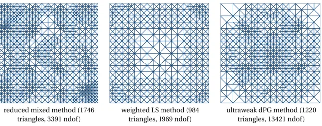
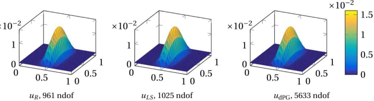
9. Numerical Experiments 80 9.1. Setup of Comparison with dPG Methods . . . 80
9.2. Square Domain with Exact Solution . . . 81
9.3. Waterfall Example . . . 86
9.4. L-Shaped Domain with Exact Solution . . . 90
9.5. Slit Domain with Exact Solution . . . 98
9.6. L-Shaped Domain with Point Load . . . 103
9.7. Discussion of Experiments . . . 108
10. Conclusion and Outlook 110 References 111 List of Tables 119 List of Figures 120 A. Remarks on the Implementation 123 A.1. Primal and Ultraweak dPG Method . . . 125
A.2. Reduced Mixed Methods . . . 127
A.3. Weighted Least-Squares Methods . . . 129
1. Introduction
This thesis analyses and proves optimal convergence rates for four lowest-order adaptive discontinuous Petrov-Galerkin (dPG) finite element methods in any space dimension for the Poisson model problem. The first part of this introduction gives a motivation and historical overview of dPG and adaptive finite element methods. The remainder of the introduction describes the discrete primal dPG method and special cases of two equivalent discrete schemes analysed in this thesis, as well as the corresponding adaptive algorithms, and elaborates on the main results of this thesis.
Motivation
Partial differential equations are a powerful tool in the description of a variety of phenomena in engineering, physics, and stochastics. A powerful tool for their numerical solution is the plethora of finite element methods with a multitude of applications ranging from automotive design to bio-engineering.
A recent asset to this family is the discontinuous Petrov-Galerkin finite element methodology introduced by L. Demkowicz and J. Gopalakrishnan [DG10; DG11a; DGN12; ZMDG+11].
Originally motivated by the construction of optimal test functions from a fixed space of trial functions [DG11b], they are characterized as a minimal residual method with a dis- continuous test space. Based on an analysis of inf-sup conditions, the dPG methodology may circumvent the cumbersome construction of balanced discrete trial and test spaces and instead provide well-posedness of the discrete problem by the choice of a sufficiently large discrete test space. Additional advantages of these methods, such as flexible mesh design, improved stability properties and a built-in error estimate [CDG14], have lead to various applications. Among the linear problems, there are publications on the Pois- son model problem [DG11b; DG13; CGHW14], linear elasticity [BDGQ12; CH16; KFD16;
FKDL17], the Stokes equations [RBD14; CP18], and the Kirchhoff-Love plate model [FHK18].
A number of papers study the convection-diffusion-reaction equations with or without singular pertubation [DG10; DGN12; DH13; CEQ14; CHBD14; BS14; BS15; FH17; HK17a;
MZ17; BDS18; Füh18]. Other applications include Maxwell’s equations [DL13; CDG16], wave propagation [DGMZ12; GMO14; PD17], the Schrödinger equation [DGNS17], the frac- tional Laplacian [ABH18] and fractional advection-diffusion [EFHK17], the heat equation [FHS17a], transmission problems [HK15; FHK17; FHKR17] and a hypersingular integral equation [HP14; HK17b]. The dPG methodology has also been applied to nonlinear model problems [CBHW18], to a contact problem [FHS17b], in nonlinear fluid mechanics [CDM14;
RDM15] and viscoelasticity [KKRE+17; FDW17].
In most of these applications, the discrete test space employs a theoretically verified [HKS14]
polynomial degree ofp+nfor the space dimensionnand the polynomial degreepof the discrete trial space. In contrast to that, [BGH14; CGHW14; CH16; CBHW18; CP18] and this
thesis analyse a lowest-order version withp=0 in the discrete trial space and degreep+1 in the discrete test space.
Several of the mentioned publications utilize the built-in error estimator [CDG14] to drive adaptive algorithms and present numerical experiments withh- andhp-adaptive refine- ment. The multitude of valuable applications of the dPG methods and their prevalent use of adaptivity make an analysis of adaptive dPG schemes desirable. However, the paper [CH18b]
presented also as part of this thesis is the first to analyse convergence and optimal rates of anh-adaptive dPG finite element method theoretically.
The need for adaptive refinement strategies arises for solutions with singularities, e.g., caused by re-entrant corners of non-convex domains or boundary conditions. The resulting reduced regularity of the exact solution [Gri11] leads to a suboptimal convergence rate for uniform refinement of the coarse initial triangulation. Whereas the possible remedy of graded meshes needs a priori knowledge of the solution, the design of adaptive refinement strategies aims at the automatic detection of those singularities and local refinement in convenient parts of the domain. Figure 1 shows an adaptively refined triangulation of an L-shaped domain with constant right-hand sidef ≡1 in the Poisson model problem calculated with the primal dPG method and its built-in error estimator.
Figure 1: Adaptively refined triangulation of L-shaped domain with singularity at the re- entrant corner.
The adaptive algorithm introduced in [Dör96] relies on the construction of a computable error estimator that is utilized for marking and then refining certain elements. However, the analysis of convergence of those adaptive algorithms is not trivial compared to that of uniform refinement strategies, since convergence of the latter is based on estimates in terms of the maximal mesh-size, which may not converge to 0 in case of adaptive refinement. In fact, while the early works on construction of error estimators with application to adaptive refinement strategies trace back to [BR78; BR81; BV84], a proof of convergence of an adaptive
algorithm in 2d was not until [Dör96; MNS00]. However, next to plain convergence of the adaptive algorithm, the main question of interest is that of rate-optimality. [BDD04]
were the first with a proof of optimal convergence rates, but they needed an additional coarsening step. The paper [Ste07] features the first proof of optimal convergence rates without coarsening and utilizes the concept of nonlinear aproximation classes. The recent contributions [CFPP14; CR17] provide an abstract axiomatic framework on the analysis of adaptive mesh-refinement able to cover various finite element methods and problems, among those the dPG methods analysed in this thesis.
For the dPG methods, the built-in a posteriori error estimate from [CDG14] provides an error estimator which is efficient and reliable up to data approximation terms and can be utilized in adaptive refinement strategies. Unfortunately, the aforementioned axiomatic approach cannot be applied to this estimator immediately due to the lack of a factor of the mesh-size hin the estimator, which leads to severe difficulties in the proof of estimator reduction. This problem is known from the least-squares (LS) methods, where [CP15] were the first to prove rate-optimality for adaptive methods for the Poisson model problem by use of an alternative error estimator. The strategy of constructing an equivalent error estimator and proving of the axioms of adaptivity for it is also employed in this thesis twice. Four lowest-order dPG methods for the Poisson model problem are shown to be equivalent to a mixed system with Crouzeix-Raviart and Courant finite element spaces, and additionally, to a generalized LS method. Both approaches lead to alternative error estimators for the four dPG methods for which the axiomatic framework of [CR17] is applicable and proves optimal convergence rates.
Problem Setting and Discrete Schemes
LetΩ⊂Rn be a bounded Lipschitz domain with polyhedral boundary∂Ω. Given a right- hand side functionf ∈L2(Ω), consider the Poisson model problem as a second-order partial differential equation that seeksu∈H1(Ω) with
−∆u=f inΩ and u=0 on∂Ω, (1.1)
or as a first-order system of equations that seeksu∈H1(Ω) andσ∈H(div,Ω) with
−divσ=f inΩ and σ= ∇uinΩ and u=0 on∂Ω. (1.2) The standard weak formulation [BBF13, p. 7] departs from (1.1) with multiplication of a test function in the Sobolev spaceH01(Ω) and and integration by parts on the domainΩand seeksu∈H01(Ω) with
∫
Ω∇u· ∇v dx=
∫
Ωf vdx for allv∈H01(Ω). (1.3)
The variational formulation beneath theprimal dPG formulation[DG13] bases on a regular triangulationT ofΩand an integration by parts of (1.1) on each finite element domain
T ∈T, which yields∫
T∇u· ∇v dx−∫
∂Tv∇u·νT ds =∫
T f vdx for anyv ∈H1(T) :={v ∈ L2(Ω)|∀T ∈T,v|T ∈H1(T)} and outer unit normalνT along∂T. The sum over allT ∈T and the introduction of the trace variablet:=(tT)T∈T withtT := ∇u·νT ∈H−1/2(∂T) lead to
b((u,t),v) := ∑
T∈T
(
∫
T∇u·∇vdx−
∫
∂Tv tT ds)
=
∫
Ω
f vdx=:F(v) for allv∈H1(T). (1.4)
A lowest-order discretization [BGH14] employs discrete spacesP1(T) of piecewise affine functions,S10(T) :=P1(T)∩H01(T) of piecewise affine, globally continuous functions with homogeneous boundary conditions and piecewise constant functionsP0(E) on the sidesE of the triangulation. For anyv1,w1∈P1(T), define the piecewise gradient by (∇NCv1)|T :=
∇(v1|T) for anyT∈T, the scalar product (v1,w1)H1(T):=(v1,w1)L2(Ω)+(∇NCv1,∇NCw1)L2(Ω), and the norm∥v1∥H1(T):=(v1,v1)1/2H1(
T). Then one characterization of the discrete dPG method is the minimization of the residual in the discrete dual norm inS01(T)×P0(E),
(uC,t0)= argmin
(wC,s0)∈S10(T)×P0(E)∥F−b((wC,s0),•)∥P1(T)∗, where (1.5)
∥F−b((wC,s0),•)∥P1(T)∗:= sup
w1∈P1(T)\{0}
|F(w1)−b((wC,s0),w1)|
∥w1∥H1(T)
.
An equivalent characterization of this discrete dPG solution is the mixed system [CDW12]
that seeks (uC,t0,v1)∈S10(T)×P0(E)×P1(T) with
(v1,w1)H1(T)+b((uC,t0),w1)=F(w1) for allw1∈P1(T),
b((wC,s0),v1)=0 for all (wC,s0)∈S10(T)×P0(E). (1.6) WhereasuC∈S10(T) is an approximation of the exact solutionu∈H01(T) andt0∈P0(E) an approximation of (∇u·νT)T∈T, the variablev1∈P1(T) is the Riesz representation of the residualF−b((uC,t0),•) inP1(T) and an approximation of the exact residual 0.
These two different notions (1.5) and (1.6) of the discrete dPG method are the starting point for the two equivalent discrete schemes introduced first for a nonlinear model problem generalizing the Poisson model problem in [CBHW18] and utilized in this thesis for the proof of optimal convergence rates.
The so-called reduced mixed system employs the piecewise affine, globally continuous functionsS10(T) as well as the Crouzeix-Raviart finite element spaceC R01(T) of piecewise affine functions that are continuous in the midpoints of inner sides and vanish on midpoints of boundary sides. Then a reasoned elimination of the element boundary terms in the approach of the dPG scheme as the mixed system of equations (1.6) leads to the equivalent reduced mixed method that seeks (vC R,uC)∈C R01(T)×S10(T) with
(∇NCvC R+ ∇uC,∇NCwC R)L2(Ω)+(vC R,wC R)L2(Ω)=(f,wC R)L2(Ω)for allwC R∈C R01(T), (∇wC,∇NCvC R)L2(Ω)=0 for allwC∈S10(T). (1.7)
The solution to this system consists of an approximationuC∈S10(T) of the exact solution u∈H01(Ω) to the weak formulation (1.3) and of an approximationvC R∈C R01(T) to the exact residual 0.
The other nonstandard discrete scheme for the Poisson model problem analysed in this thesis, theweighted LS method, departs from the point of view of the primal dPG method as a minimal residual method (1.5) and generalizes standard LS finite element schemes. It considers mesh-dependent piecewise constant weight functionsS(T)∈P0(T;Rn×n) and the space of Raviart-Thomas finite element functionsRT0(T) consisting of certainH(div)- conforming functions in the space of piecewise affine vector fields. Then a direct calculation of the discrete dual norm∥F−b((wC,s0),•)∥P1(T)∗with an extension of the trace variable s0to a unique qRT ∈RT0(T) leads to an equivalent weighted LS method that seeks the minimizer
(pLS,uLS)= argmin
(qRT,wC)∈RT0(T)×S10(T)
(∥Π0f +divqRT∥2L2(Ω)+ +
(In×n+S(T))−1/2(Π0qRT− ∇vC+Π0(f(id−mid(T))))2L2(Ω)).
(1.8)
Here,uLS∈S10(T) approximates the exact solutionu∈H01(Ω) andpLS ∈RT0(T) approxi- mates∇u∈H(div,Ω).
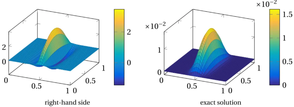
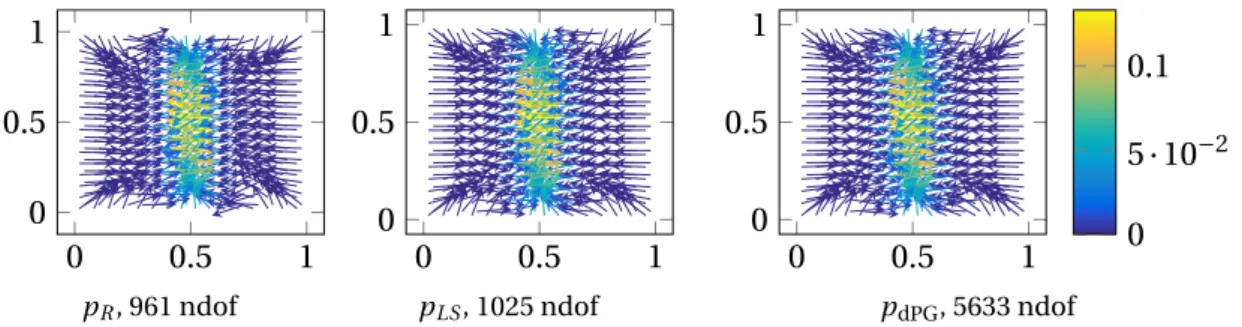
Figures 2-4 display the parts of the discrete solutions of the primal dPG method (1.6), the reduced mixed method (1.7), and of the weighted LS method (1.8) and illustrate their equivalence on a uniform triangulation of an L-shaped domain with 384 triangles for a constant right-hand sidef ≡1.
−1 0 1−1 0 1 0
0.1
uC∈S10(T)
−1 0 1
−1 0 1
0.2 0.4 0.6
t0∈P0(E)
−1 0 1−1 0 1 0
2 4
×10−2
v1∈P1(T)
Figure 2: Solution plots of primal dPG scheme (1.6) with 1921 degrees of freedom, where t0∈P0(E) is visualized by a quiver plot of its unique extensionpRT∈RT0(T).
−1 0 1−1 0 1 0
0.1
uC∈S10(T)
−1 0 1−1 0 1 0
2 4
×10−2
vC R∈C R01(T)
Figure 3: Solution plots of reduced mixed scheme (1.7) with 705 degrees of freedom.
−1 0 1−1 0 1 0
0.1
uLS∈S10(T)
−1 0 1
−1 0 1
0.2 0.4 0.6
pLS∈RT0(T)
Figure 4: Solution plots of weighted LS scheme (1.8) with 769 degrees of freedom.
The primal dPG method and the reduced mixed method utilize the standard adaptive finite element loop visualized in Figure 5.
SOLVE ESTIMATE MARK REFINE
Figure 5: Standard adaptive loop for collective marking.
This means that after the discrete solution on a triangulationT, the stepestimatecomputes an error estimatorη(T,T)≥0 for any simplexT ∈T andη(T) :=(∑
T∈Tη(T,T)2)1/2. Based on this refinement indicator, the standard adaptive algorithm employs collective marking, also called Doerfler marking [Dör96], to select simplices which are then refined in the last step of the loop.
The adaptive algorithm with separate marking is needed for the weighted LS method, since its a posteriori error estimate contains an additional data approximation termµ(T)≥0. If the estimatorη(T,T) dominatesµ(T), the loop utilizes collective marking as before. In the other case, a data approximation algorithm leads to a new triangulation with a reduced µ(T). Figure 6 illustrates the adaptive finite element loop with separate marking.
SOLVE ESTIMATE
MARK REFINE
MARK REFINE
MARK REFINEXX APPROX
Figure 6: Adaptive loop for separate marking.
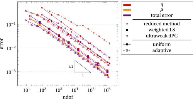
The analysis of convergence and rate-optimality of these adaptive algorithms is possible through a framework [CFPP14; CR17] consisting of axioms (A1), (A2), (A3), (A4), and (QM) that concern the error estimators and some distance function. A proof of these axioms implies optimal convergence rates of the estimator in terms of the degrees of freedom for the output (Tℓ)ℓ∈N0of the adaptive algorithm, i.e., that anys>0 satisfies
sup
ℓ∈N0
(1+ |Tℓ| − |T0|)sη(Tℓ)≈ sup
N∈N0
(1+N)smin{η(T)|T ∈Twith|T| − |T0| ≤N}. (1.9)
Figure 7 illustrates this notion of rate-optimality with a convergence history plot of an adaptive primal lowest-order dPG method for the Poisson model problem on the non- convex slit domain for a constant right-hand side f ≡1. It shows that whereas the re- entrant corner of the domain leads to the suboptimal convergence rate 0.3 for uniform refinement, the convergence ratesof the adaptive scheme is 0.5, which is the optimal rate for approximation with this polynomial degree. The crosses symbolize the (not computed) optimal triangulations in terms of the error estimators with respect to the number of degrees of freedom of the right-hand side of (1.9).
102 103 104 105 106 10−2
10−1 100
1 0.3
1/2
1
ndof
errorestimator
error estimator uniform error estimator adaptive error estimator optimal (symbolic)
Figure 7: Convergence history plot of error estimators for primal dPG method on slit domain with right-hand sidef ≡1.
Main Results
This thesis proves optimal convergence rates for four lowest-order dPG methods for the Poisson model problem for a sufficiently small initial mesh-size in two different ways by equivalences to two other types of methods, the reduced mixed and the weighted LS meth- ods.
A main step to prove rate-optimality is the characterization of all four dPG methods as particular instances of these two methods. This is a major generalization of the equivalence developed in [CBHW18] only for the primal dPG method. In order to treat all four dPG methods simultaneously, the reduced mixed and the weighted LS method from [CBHW18]
described in this introduction are equipped with more general parameters and weights, in- cluding but not restricted to those that lead to the four different dPG methods. Assumptions on these parameters and weights were derived as general as possible to include as many as possible different methods, but still guaranteeing well-posedness and eventually also rate-optimality of the adaptive alogorithm.
Since this shows that all properties, e.g., optimal convergence rates, of the four dPG methods follow as special cases from the respective properties of the reduced mixed or the weighted least-squares methods, this thesis then focuses on the analysis of these two methods for general parameters and weights.
The first important result in the analysis of the adaptive reduced mixed and weighted LS methods is the derivation of reliable and efficient computable error estimators. Both estimators utilize residual error estimators with volume terms and jump terms along the sides, both weighted with factors of the mesh-sizeh. An important tool in the construction of both estimators is the equivalence
∥∇NCwC R∥2L2(Ω)≈ ∑
E∈E(Ω)|E|1/(n−1)∥[∇NCwC R]E∥2L2(E)
developed in this thesis for Crouzeix-Raviart functionswC R ∈C R10(T) that satisfy theL2 orthogonality∇NCwC R ⊥ ∇S10(T). The error estimator for the weighted LS method has an additional data approximation error term∥(1−Π0)f∥L2(Ω), which causes the need for separate instead of collective marking in the adaptive algorithm for this method.
Whereas the proofs of the axioms of stability (A1) and reduction (A2) for both methods follow standard arguments, the proofs of discrete reliability (A3) and quasi-orthogonality (A4) are essential achievements of this thesis.
The proof of discrete reliablity for the reduced mixed method subtly combines tools of the dis- crete reliability for the Crouzeix-Raviart method, in particular, a discrete quasi-interpolation operator from [CGS13] and introduces some nonconforming energies as auxiliary variables.
The quasi-orthogonality (A4) is proved in form of some quasi-orthogonality with a small parameterε, which leads to (A4) for a sufficiently fine initial triangulation. This condition is needed for the proof of quasi-monotonicity (QM) as well and finally leads to the statement of optimal convergence rates for the reduced mixed methods.
In contrast to the reduced mixed methods, the axiom of quasi-monotonicity (QM) for the weighted LS methods does not need the condition of a sufficiently small initial mesh-size.
The analysis of discrete reliablity (A3) for the weighted LS methods follows the strategy prescribed for the standard LS method in [CP15], but with some extra technical difficulties caused by the weight functions that differ from triangulation to triangulation. A central lemma for overcoming this problem estimates the error of differently weighted vector fields by a difference of the eigenvalues of the matrix-valued weights. Furthermore, an insight gained from the connection of these weighted LS methods to the reduced mixed methods enabled the proof of discrete reliability without a discrete Helmholtz decomposition, which therefore holds in any space dimension as compared to onlyn=2 in [CP15]. The proof of quasi-orthogonality with a parameterεalso relies on the estimation of the weights. This leads to the main result of optimal convergence rates with the separate marking adaptive algorithm for the weighted LS methods.
All proofs gather explicit constants in the spirit of [CH18a], sometimes subsumed within the proofs for the sake of readability. Table 1 gives an overview of constants employed in the proofs with references.
The numerical experiments of this thesis verify the optimal convergence rates of both types of methods for different choices of parameters. Moreover, they complement the theory by a thorough comparison of both methods among each other and with their equivalent dPG schemes.
Outline of this thesis
The remainder of this thesis is organized as follows. Section 2 gives a detailed introduction into the notation and tools employed in this thesis. It starts with a recapitulation on func- tion spaces, triangulations, refinements and the set of admissible triangulations. It then introduces the adaptive algorithms and the axioms of adaptivity. Afterwards, it summarizes the existing literature on the abstract framework of dPG methods and the trace operators essential to them. The section concludes with a collection of important tools, inequalities and interpolation operators utilized in this thesis.
The main part of this thesis consists of Sections 3-8, which is basically divided into two parts of analogous structure. The first part analyses the reduced mixed method and is a more detailed exposition of [CH18b], whereas the second part contains the analysis of the weighted LS method, which is yet unpublished. Section 3 introduces the reduced mixed method, proves well-posedness thereof, derives an efficient and reliable error estimator and states a number of abstract assumptions on the parameters of the method. Section 4 inserts the four lowest-order dPG methods into this framework by proving equivalence to the reduced mixed scheme for different choices of parameters. Finally, Section 5 proves the axioms of adaptivity (A1)-(A4) and all intermediate steps needed for them and deduces the statement of quasi-monotonicity (QM) and therefore, rate-optimality in a summarising theorem.
Constant Reference
csr shape regularity Definition 2.14 on p. 17
cdF,cF (discrete) Friedrichs inequality Theorems 2.28, 2.29 on p. 23 cdP,cP (discrete) Poincaré inequality Theorem 2.30 on p. 24
cinv inverse inequality Theorem 2.31 on p. 24
cdtr,ctr (discrete) trace inequality Lemma 2.33, Remark 2.34 on p. 24 κNC nonconforming interpolation opera-
tor
Theorem 2.36 on p. 25 capx(Jk) conforming companion operator Theorem 2.37 on p. 25 cdQI discrete quasi interpolation Theorem 2.38 on p. 26 cdCR discrete quasi interpolation for CR Theorem 2.39 on p. 26 cjc discrete jump control [CR17, Lem. 5.2]
cQ approximation property ofQ Assumption (3.5) on p. 30 crel,ceff reliability and efficiency for reduced
mixed method
Corollary 3.3 on p. 30 cLS standard LS equivalence (6.3) on p. 53
λ,λ uniform boundedness ofM0 Assumption (6.6) on p. 54
κ1 boundedness ofF0 Assumption (6.7) on p. 54
crel,ceff reliability and efficiency for weighted LS method
Lemma 6.7 on p. 58
Λ1 Stability (A1) Subsection 2.4, Thm. 5.1 on p. 42,
and Thm. 8.2 on p. 68
Λ2,ϱ2 Reduction (A2) Subsection 2.4, Thm. 5.2 on p. 42, and Thm. 8.3 on p. 69
Λ3,Λˆ3 Discrete reliability (A3) Subsection 2.4, Thm. 5.5 on p. 45, and Thm. 8.10 on p. 73
Λ4 Quasiorthogonality (A4) Subsection 2.4, Thm. 5.8 on p. 49, and Thm. 8.13 on p. 78
ΛQM Quasiomonotonicity (QM) Subsection 2.4 and Thm. 8.1 on p. 67 Table 1: Overview of constants in this thesis
The structure of Sections 6-8 for the weighted LS method is similar. The introduction of the method and its error estimator, its stability, and the general assumptions on the weights are contained in Section 6. It is followed by Section 7 with proofs of equivalence of the four dPG methods to the weighted LS method for certain choices of the weights. Section 8 proves the axioms of adaptivity (QM) and (A1)-(A4) and gives the resulting statement of optimal convergence rates. Sections 3, 5, 6, and 8 treat the analysis of the reduced mixed method and the weighted LS method and can be read independently of previous knowledge of dPG methods.
Section 9 presents numerical experiments on five benchmark examples, four of which have known exact solutions. It includes a variety of convergence history plots, solution plots, triangulations and tables examining optimal convergence rates and illustrating equivalence of the methods. A special focus is on the examination of the computational differences between the theoretically equivalent methods, including a study of computation times.
The thesis closes with a conclusion of the achieved results and an outlook of future research in Section 10.
Appendix A comments on the software attached to this thesis and utilized for the numerical experiments.
Acknowledgements
As the writing of a PhD thesis involves more than just one person, I want to take the opportu- nity to appreciate the help and support of several people. First of all, there is my supervisor Prof. Carstensen, who has accompanied my scientific development for several years by now.
I am very grateful to him for teaching me so much about numerical analysis and mathemati- cal writing, and for supporting my career. Next to that, I want to thank my working group and my colleagues all across the world, for all the great experiences at various scientific events and all the knowledge they shared with me. Furthermore, thank you to the The Berlin Mathematical School and the Deutsche Forschungsgemeinschaft in the Priority Program 1748 “Reliable simulation techniques in solid mechanics. Development of non-standard discretization methods, mechanical and mathematical analysis” (CA 151/22-1) for their financial support.
What is more, I want to express my gratitude to my friends and family for always being there, for always listening to me, having my back and also for taking my mind off work if necessary.
My friend and colleague Philipp occupies a special place in the intersection of different areas of my life. I cannot thank you enough for your highly appreciated thoughts on mathematics and everything else, for your diverse help, and for being such a good company over the years of our friendship and as colleagues. Last but not least – Nino and Stevie. You are invaluable to me, each of you in their individual way, and I am beyond grateful for having you in my life.
Your love and support keep me going.
Space Reference Ck(Ω) ktimes continuously differentiable functions [Alt16, p. 43]
C∞(Ω) :=⋂
k∈N0Ck(Ω) [Alt16, p. 45]
Cc∞(Ω) :={f ∈C∞(Ω)|supp(f)⊆Ωcompact} [Eva10, p. 242]
Lp(Ω) Lebesgue functions Definition 2.1
H1(Ω) Sobolev space of functions with weak derivative Definition 2.3 H01(Ω) Sobolev space with zero boundary condition Definition 2.3 H(div,Ω) functions with weak divergence Definition 2.4 H1/2(∂T) traces of Sobolev functions on skeleton Definition 2.20 H−1/2(∂T) normal traces ofH(div) functions on skeleton Definition 2.20 H1(T) piecewise Sobolev functions Definition 2.5 HNC1 (T) piecewise Sobolev functions with jump condition Definition 2.7
Table 2: Overview of continuous function spaces, all discrete spaces in Subsection 2.2
2. Notation and Preliminaries
Throughout this thesis, consider a polyhedral, bounded Lipschitz domain [Gri11, p. 5-7]
Ω⊂Rn with boundary∂Ωforn=2,3. Denote the Euclidean scalar producta·b and the tensor producta⊗b:=ab⊤∈Rℓ×ℓof two vectorsa,b∈Rℓ,ℓ∈Nand the symmetric matrices S⊂Rℓ×ℓ. The measure|•|is context-sensitive and refers to the modulus (a·a)1/2of a scalar or vectora∈Rℓ, the number of elements of some finite set or the Lebesgue measure|ω| of a Lebesgue measurable setω⊂Rn. Denote the identity mapping •=id and the identity matrixIn×n∈S.
2.1. Function Spaces
This section recalls the standard notation on Lebesgue and Sobolev spaces summarized in Table 2.
Definition 2.1 (Lebesgue spaces [Alt16, pp. 50 ff.]) For 1≤p≤ ∞,Lp(Ω) denotes the space of Lebesgue functionsΩwith norm∥f∥Lp(Ω)=(∫
Ω|f|p dx)1/pfor 1≤p< ∞and∥f(x)∥L∞(Ω)= esssupx∈Ω|f(x)|. For setsU ⊆R,U ⊆Rℓ, orU ⊆Rℓ×m, ℓ,m ∈N, Lp(Ω;U) denotes the Lebesgue functions onΩwith values inU. For functionsf,g∈L2(Ω;U),U⊆Rℓ,ℓ∈N, the L2scalar product reads (f,g)L2(Ω):=∫
Ωf ·g dx.
Remark 2.2 For ease of notation, most of the definitions in the remainder of this chapter fo- cus on scalar valued functions. However, the definitions of operators apply componentwise to vector- or matrixvalued functions as well and are denoted with the same variable. In case of function spaces, the “;U” in the name of the space like in Definition 2.1 above or in the discrete spaces of Definition 2.6 below indicates the rangeU⊆R,Rℓ,Rℓ×m,ℓ,m∈N, of the functions.
Definition 2.3 (Weak derivative, Sobolev space [Eva10, p. 245]) For anyj∈{1,...,n} and a functionv∈L2(Ω), thejthweak partial derivative∂v/∂xj ofv is a functionw:Ω→Rthat satisfies∫
Ωv∂ϕ/∂xj dx= −∫
Ωwϕdxfor anyϕ∈Cc∞(Ω) [Eva10, p. 245]. The gradient ofv is the column vector∇v=(∂v/∂x1,...,∂v/∂xn)⊤. The Sobolev space
H1(Ω) :={v∈L2(Ω)|∇v exists in a weak sense and∇v∈L2(Ω;Rn)}
employs the norm∥v∥2H1(Ω):= ∥v∥2L2(Ω)+ ∥∇v∥2L2(Ω)for anyv∈H1(Ω). In the sense of traces defined in Theorem 2.18 in Subsection 2.5 below, define the space
H01(Ω) :={v∈H1(Ω)|v=0 almost everywhere along∂Ω}
with norm|||v|||:= ∥∇v∥L2(Ω)for anyv∈H01(Ω).
Next to functions with weak derivative, this thesis employs functions with weak divergence.
Definition 2.4 (H(div) space [BBF13, p. 49]) For any q ∈L2(Ω;Rn), the weak divergence divqofqis a functionw:Ω→Rthat satisfies∫
Ωu· ∇ϕdx= −∫
Ωwϕdxfor anyϕ∈Cc∞(Ω).
Define
H(div,Ω) :={q∈L2(Ω;Rn)|divqexists in a weak sense and divq∈L2(Ω)}
with norm∥q∥2H(div):= ∥q∥2L2(Ω)+ ∥divq∥2L2(Ω)for anyq∈H(div,Ω).
Definition 2.5 (Piecewise Sobolev andH(div) space) Given a triangulation T of the do- mainΩ, define the piecewiseH1andH(div) spaces by
H1(T) :={vT ∈L2(Ω)|∀T ∈T,vT|T ∈H1(T)}, H(div,T) :={qT ∈L2(Ω;Rn)|∀T∈T,qT|T ∈H(div,T)}.
Furthermore, define the piecewise weak gradient∇NC for any vT ∈H1(T) and T ∈T by (∇NCvT)|T := ∇(vT|T) and the piecewise weak divergence divNC by (divNCqT)|T := div(qT|T) for anyqT ∈H1(T). With|||•|||NC:= ∥∇NC•∥2L2(Ω)onH1(T), the norms on these spaces read
∥vT∥2H1(T):= ∥vT∥2L2(Ω)+ |||vT|||2NC for anyvT ∈H1(T),
∥qT∥2H(div,NC):= ∥qT∥2L2(Ω)+ ∥divNCqT∥2L2(Ω) for anyqT ∈H(div,T).
Define the bilinear formaNC(vT,wT) :=(∇NCvT,∇NCwT)L2(Ω)for anyvT,wT ∈H1(T).
2.2. Triangulation and Discrete Spaces
For anyn-simplexT =conv{z1,...,zn+1}⊆Rn,N(T)={z1,...,zn+1} denotes its nodes and E(T) its sides. Similarly, for a regular triangulation T of the domain Ω into simplices [Cia02, p. 38], let N =⋃
T∈TN(T) (resp. N(Ω) resp. N(∂Ω)) the set of all nodes (resp.
νE νT+ νT+
νT+ νT−
νT−
νT− T+ E
T−
νE νT+ νT+
νT+ T+ E
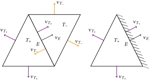
Figure 8: Side patchωE and normal vectors for an inner side and a boundary side in 2d inner nodes resp. boundary nodes) andE=⋃
T∈T E(T) (resp. E(Ω) resp. E(∂Ω)) the set of all sides (resp. inner sides resp. boundary sides). For any simplexT ∈T, denote the patchωT =⋃
K∈T,N(T)∩N(K)̸=;K. Furthermore, define the skeleton of a triangulation by
∂T :=⋃
T∈T⋃
E∈E(T)E.
LetνT the outer unit normal vector along the boundary∂T of a simplexT. For any inner sideE=∂T+∩∂T−∈E(Ω) as in Figure 8, denote the side patchωE=int(T+∪T−) and fix one of the two possible directions of the unit normal vectorνE of the side and thus, the notation of the neighboring elementsT+andT−viaνT+|E=νE. For a boundary edgeE∈E(∂Ω) with E=∂T∩∂Ω, letωE =T and the unit normal vectorνE of the side point outwards.
Define the jump ofv∈H1(T) by [v]E :=v|T+−v|T−∈L2(E) on any inner sideE∈E(Ω) and by [v]E:=v∈L2(E) on any boundary sideE∈E(∂Ω). For anyv∈L2(E), define the integral mean∫−
Evds:=∫
Ev ds/|E|along the side. The side normalsνE= ±νT±from above generate jumps in that anyv∈H1(T) satisfies
∑
T∈T
∫
∂TvνT ds= ∑
E∈E
∫
E[v]EνE ds. (2.1)
Consider the midpoint mid(T) :=1/(n+1)∑
z∈N(T)z, diameterhT :=supx,y∈T|x−y|, and the Lebesgue measureHT := |T|1/nof any simplexT and the corresponding piecewise constant functions mid(T),hT, andHT defined by mid(T)|T :=mid(T),hT|T :=hT, andHT|T :=HT
for anyT ∈T. These satisfy the pointwise estimate|•−mid(T)| ≤nhT/(n+1).
Definition 2.6 (Piecewise polynomials) The piecewise polynomials of degreek∈N0read Pk(T) :={vk∈L∞(T)|vkalgebraic polynomial onT of total degree ≤k},
Pk(T) :={vk∈L∞(Ω)| ∀T ∈T,vk|T ∈Pk(T)},
Pk(T;U) :={qk∈L∞(T;U)|each component ofqkis inPk(T)}, forU⊆R,Rℓ, orRℓ×m, Pk(T;U) :={qk∈L∞(Ω;U)| ∀T ∈T,vk|T ∈Pk(T;U)}.
Analogously, define piecewise polynomials on edges,
Pk(E) :={vk∈L∞(E)|vkalgebraic polynomial onE of total degree ≤k}, Pk(E) :={vk∈L∞(E)| ∀E∈E,vk|E ∈Pk(E)}.
The following classical finite element spaces trace back to [Cou43; CR73; RT77] and employ piecewise polynomials with some additional continuity and boundary conditions.
Definition 2.7 (Finite element spaces) For anyk∈N0, define the conforming spaces Sk0(T) :=Pk(T)∩H01(Ω)⊆Sk(T) :=Pk(T)∩H1(Ω).
The Crouzeix-Raviart functions form a subspace ofHNC1 (T), where HNC1 (T) :={vT ∈H1(T)|∀E∈E(Ω),−
∫
E[vT]E ds=0},
C R1(T) :={vC R∈P1(T)|∀E∈E(Ω), vC Rcontinuous at mid(E)}⊆HNC1 (T), C R01(T) :={vC R∈C R1(T)|∀E∈E(∂Ω), vC R(mid(E))=0}.
The (piecewise) lowest-order Raviart-Thomas functions read
RT0NC(T) :={q1∈L∞(Ω;Rn)|∃A∈P0(T;Rn),b∈P0(T),q1=A+b(• −mid(T))}, RT0(T) :=RT0NC(T)∩H(div,Ω).
Definition 2.8 (Galerkin projection) Define the linear and bounded operatorG:H1(T)→ S10(T) byGvT :=vC for anyvT ∈H1(T) and the uniquevC∈S10(T) that satisfies
∫
Ω∇vC· ∇wC dx=
∫
Ω∇NCvT· ∇wCdx for allwC∈S10(T).
For properties of the subsequently definedL2projectionΠksee Lemma 2.24 below.
Definition 2.9 (L2projection and oscillations) For any k ∈N0, define theL2 projection Πk:L2(Ω)→Pk(T) uniquely for anyv∈L2(Ω) via ((1−Πk)v,vk)L2(Ω)=0 for anyvk∈Pk(T).
Furthermore, define the oscillation osc(f,T) := ∥hT(f −Π0f)∥L2(Ω).
The following piecewise constant functions are weights of the dPG methods in the context of the weighted least-squares formulation from Section 6.
Definition 2.10 (Weights) Define the piecewise constant mappingsS(T)∈P0(T;S),s(T)∈ P0(T) and the operatorH0:L2(Ω)→P0(T;Rn) by
S(T) :=Π0((•−mid(T))⊗(•−mid(T))), s(T) :=trS(T)=Π0|•−mid(T)|2,
H0f :=Π0(f(•−mid(T))) for anyf ∈L2(Ω).
Remark 2.11 (P1(T) andRTNC
0 (T)) Anyv1∈P1(T) andq1∈RT0NC(T) satisfy v1=Π0v1+ ∇NCv1·(•−mid(T)) and q1=Π0q1+divNCq1(•−mid(T))/n.
This and the orthogonality of id−mid(T)=(1−Π0)id ontoP0(T) lead to an alternative representation of norms
∥v1∥2H1(T)= ∥Π0v1∥2L2(Ω)+ ∥(1+S(T))1/2∇NCv1∥2L2(Ω),
∥q1∥2H(div,NC)= ∥Π0q1∥2L2(Ω)+ ∥(1+s(T)/n2)1/2divNCq1∥2L2(Ω).
2.3. Refinement
Anyn-simplexT =conv{P1,...,Pn+1} is identified with the (n+1)-tuple (P1,...,Pn+1). Its refinement edge is P1Pn+1 and bisec(T) := {T1,T2} is defined with T1 := conv{P1,(P1+ Pn+1)/2,P2,...,Pn} andT2:=conv{Pn+1,(P1+Pn+1)/2,P2,...,Pn}. The ordering of the nodes in the (n+1)-tuples corresponding toT1andT2and thus, the refinement edges, for the new simplicesT1andT2are fixed and forn=3 additionally depend on the type of the (tagged) n-simplex [Tra97; Ste08].
For any triangulationT, a refinementTˆ is defined as a regular triangulation such that, for anyT ∈Tˆ, there existsK ∈T such thatT ⊆K. The notationT ∩Tˆ refers to simplices that are both inT and inTˆ, i.e., that have not been refined. In a similar manner, T\Tˆ denotes simplices in the coarse triangulationT that are refined, i.e., simplices before the refinement. DenoteTˆ\T the simplices in the fine triangulationTˆ that have been refined, i.e., simplices after the refinement. Given someT and a refinementTˆ, this thesis often utilizes properties or quantitiesxandxˆto symbolyze the respective relation to these two generic triangulations.
Given a regular triangulationT and an arbitrary setM⊆T of marked simplices, thenewest vertex bisectionalgorithm [Mit89; Ste08] bases on a successive bisection of simplices and generates a minimal refinementTˆ ofT such that the marked simplices are refined, i.e., M⊆T \Tˆ. Strictly speaking, the newest vertex bisection requires a tagged simplex and the initialization requires an initial condition [Ste08, §4] suppressed here for simplicity of notation.
Definition 2.12 Given a regular initial triangulationT0, define theadmissible triangulations T:={T|T is refinement ofT0by a sequence of newest vertex bisections}.
Furthermore, givenT ∈T, define the set of admissible refinements ofT by
T(T) :={Tˆ|Tˆ is refinement ofT by a sequence of newest vertex bisections}.
The set of admissible simplices reads⋃T=⋃
T∈TT. For anyK ∈T ∈Tand a refinement Tˆ ∈T(T), define Tˆ(K) :={T ∈Tˆ|T ⊆K}. Furthermore, for δ>0, denoteT(δ)={T ∈ T|hT ≤δa.e. inΩ}. The maximal mesh sizehmax :=maxT∈TmaxT∈ThT is bounded by h0:=maxT∈T0hT ≤diam(Ω).