A Sub-Element Adaptive Shock Capturing Approach for Discontin- uous Galerkin Methods

Center for Data and Simulation Science

Johannes Markert, Gregor Gassner, Stefanie Walch

A Sub-Element Adaptive Shock Capturing Approach for Discontin- uous Galerkin Methods

Technical Report ID: CDS-2020-10

Available at https://kups.ub.uni-koeln.de/id/eprint/25054

Submitted on November 6, 2020

FOR D ISCONTINUOUS G ALERKIN M ETHODS

Preprint submitted to Communications on Applied Mathematics and Computation.

Johannes Markert jmarkert@math.uni-koeln.de

Department for Mathematics and Computer Science, University of Cologne, Weyertal 86-90, 50931, Cologne, Germany

Gregor Gassner

Department for Mathematics and Computer Science;

Center for Data and Simulation Science,

University of Cologne, Weyertal 86-90, 50931, Cologne, Germany Stefanie Walch

Universit¨at zu K¨oln, Z¨ulpicher Str. 77, I. Physikalisches Institut;

Center for Data and Simulation Science, 50937 K¨oln, Germany

November 6, 2020

A

In this paper, a new strategy for a sub-element based shock capturing for discontinuous Galerkin (DG) approximations is presented. The idea is to interpret a DG element as a collection of data and construct a hierarchy of low to high order discretizations on this set of data, including a first order finite volume scheme up to the full order DG scheme. The different DG discretizations are then blended according to sub-element troubled cell indicators, resulting in a final discretization that adaptively blends from low to high order within a single DG element. The goal is to retain as much high order accuracy as possible, even in simulations with very strong shocks, as e.g. presented in the Sedov test. The framework retains the locality of the standard DG scheme and is hence well suited for a combination with adaptive mesh refinement and parallel computing. The numerical tests demonstrate the sub-element adaptive behavior of the new shock capturing approach and its high accuracy.

1 Introduction

For non-linear hyperbolic problems, such as the compressible Euler equations, there are two major sources of instabil- ities when applying discontinuous Galerkin (DG) methods as a high order spatial discretization. (i) Aliasing is caused by under-resolution of e.g. turbulent vortical structures and can lead to instabilities that may even crash the code. As a cure, de-aliasing mechanisms are introduced in the DG methodology based on e.g. filtering [31, 30], polynomial de-aliasing [37, 58, 38] or analytical integration [32, 26], split forms of the non-linear terms that for instance preserve kinetic energy [62, 23, 25, 18], and entropy stability [5, 61, 48, 7, 47, 45, 6, 46, 44, 3, 27, 22, 20]. (ii) The second ma- jor source of instabilities is the Gibbs phenomenon, i.e. oscillations at discontinuities. It is well known that solutions of non-linear hyperbolic problems may develop discontinuities in finite time, so called shocks. While aliasing issues can be mostly attributed to variational crimes, i.e. a bad design and implementation of the numerical discretization with simplifications that affects aliasing (e.g. collocation), oscillations at discontinuities have their root deeper in the innards of the high order DG approach and are unfortunately an inherent property of the high order polynomial ap- proximation space. Oscillations are fatal when physical constraints and bounds on the solution exist that then break because of over- and undershoots, resulting in nonphysical solutions such as negative density or pressure.

In this work, we focus on a remedy for the second major stability issue, often referred to as shock capturing. There are many shock capturing approaches available in DG literature, for instance based on slope limiters [11, 10, 41] or (H)WENO limiters [28, 51, 66], filtering [2], and artificial viscosity [49, 9]. Slope limiters or (H)WENO limiters are always applied in combination with troubled cell indicators that detect shocks and only flag the DG elements that are affected by oscillations. Only in these elements, the DG polynomial is replaced by an oscillation free reconstruction using data from neighboring elements. Element based slope limiting, e.g., with TVB limiters is effective for low order DG discretizations only, as its accuracy strongly degrades when increasing the polynomial orderN, as in some sense the size of the DG elements xgets larger and larger with higher polynomial degreeN. The accuracy of the slope limiters is not based on the DG resolution⇠ N^x, but only on the element size x. Considering that a finite volume (FV) discretization with high order reconstructions and limiters typically resolve a shock within about 2-3 cells, the shock width for high order DG schemes with large elements would be very wide when relying on element based limited reconstructions. The same behavior is still an issue for high order reconstruction based limiters such as the (H)WENO methodology. While these formally use high order reconstructions, its leading discretization parameter is still xand not _N^xand hence the shock width still scales with x.

Sub-element resolution, i.e. a numerical shock width that scales proportional to _N^x, can be achieved with e.g. artificial viscosity. The idea is to widen the discontinuity into a sharp, but smooth profile such that high order polynomials can resolve it. Again, some form of troubled cell indicator is introduced to not only flag the element that contains the shock (or that oscillates) but also determine the amount of necessary viscosity, e.g., based on local entropy production [67].

It is interesting that less viscosity is needed, i.e. sharper shock profiles are possible, the higher the polynomial degree of the DG discretization. Shocks can be captured in a single DG element if the polynomial order is high enough [49].

An issue of artificial dissipation is that a high amount of artificial viscosity is needed for very strong shocks, which makes the overall discretization very stiff with a very small explicit time step restriction. Local time stepping can be used to reduce this issue [24] or specialized many stage Runge-Kutta schemes with optimized coefficients for strongly dissipative operators [33].

An alternative idea to achieve sub-element resolution is to actually replace the elements by sub-elements (lower order DG on finer grid) or maybe even finite volume (FV) subcells. A straight forward, maybe even a natural idea in the DG methodology is to use hp-adaptivity, where the polynomial degree is reduced and simultaneously the grid resolution is increased close to discontinuities. When switching to the lowest order DG, i.e a first order DG, which is nothing but a first order FV method, it is assumed that the inherent artificial dissipation of the first order FV scheme is enough to clear all oscillations at even the strongest shocks. The low accuracy of the first order FV method is compensated by a respective (very strong) increase in local grid resolution through h-adaptivity. An obvious downside to the hp- adaptivity approach is the strong dynamic change of the approximation space during the simulation and the associated strong change of the underlying data structures.

Thus, as a simpler alternative, subcell based FV discretizations with a first order, second order TVD or high order WENO reconstruction was introduced, e.g., in [60, 57, 15, 63, 14]. The idea is to completely switch the troubled DG element to a robust FV discretization on a fine subcell grid. This approach keeps the change of the data local to the affected DG element and helps to streamline the implementation. The robust and essential oscillation free FV scheme on the finer subcell grid in the DG element is constructed based on the available DG data. This helps to keep the data structures feasible and reduces the shock capturing again to an element local technique instead of changing the global mesh topology and approximation space. Consequently, this again allows to combine the approach with the idea of a troubled cell mechanism to identify the oscillatory DG elements and replace the high order DG update with the robust FV update. As noted, there are many different variants for the FV subcell scheme with the high order WENO [60, 57, 15, 63, 14] variant being especially interesting, as it alleviates the ’stress’ on the troubled cell indicator. When accidentally switching the whole high order DG element to the subcell FV scheme in smooth parts of the solution, accuracy may strongly degrade. A first order FV scheme, even on the fine subcell grid, would wash away all fine structure details that the high order DG approach simulated. Thus, from this point of view, a high order subcell WENO FV scheme is highly desired in this context. A downside of a subcell WENO FV scheme is the non-locality of the data dependence due to the high order reconstruction stencils. This is especially cumbersome close to the interface of the high order DG elements, where the reconstruction stencils reach into the neighboring DG elements and thus fundamentally change the data dependency footprint of the resulting implementation, that consequently has a direct impact on the parallelization of the code.

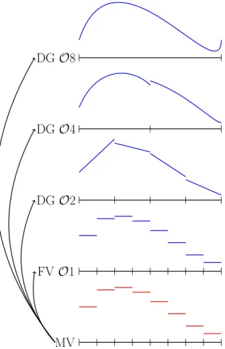
In this paper, the goal is to augment a high order DG method with sub-element shock capturing capabilities to allow the robust simulation of highly supersonic turbulent flows which feature strong shocks, as e.g. in astrophysics, without changing the data dependency footprint. Instead of flagging an element and completely switching from the high order DG scheme to the subcell FV scheme, we aim to smoothly combine different schemes in the flagged element. To achieve this, we firstly interpret the DG element as a collection of available mean value data. As depicted in Fig.1, local reconstructions allow to define a hierarchy of approximation spaces, from pure piecewise constant approximations

(subcell FV) up to a smooth global high order polynomial (DG element), with all piecewise polynomial combinations (sub-element DG) in between. We then associate each possible approximation space with the corresponding FV or DG discretization to define a hierarchy of schemes that is available for the given collection of data.

MV FV O 1 DG O 2 DG O 4 DG O 8

Figure 1: Sketch of the main idea in a one-dimensional setting. Starting with eight mean values (red), we interpret them as a collection of available data. We construct four different approximation spaces (blue): piecewise constant on a subcell grid, piecewise linear and piecewise cubic on a sub-element grid, and the full 7th degree polynomial on the element.

Instead of switching between these different schemes, we aim to smoothly blend them in order to achieve the highest possible accuracy in every DG element. Assuming that the first order subcell FV approximation has enough inherent dissipation to capture shocks in an oscillation free manner, the goal is to give the FV discretization a high enough weight at a shock and then smoothly transition to higher order (sub-element) DG away from the shock. In contrast to the common approaches, where one indicator is used for the whole DG element, we aim to introduce sub-element indicators that are adaptively adjusted inside the DG element. A difficulty that arises when using sub-element indica- tors and an adaptive blending approach is to retain conservation of the final discretization for arbitrary combinations of blending weights.

The final discretization is a blended scheme, where the weights of the different discretizations may vary inside the DG element. To demonstrate this idea, the resulting behavior of the new approach is depicted in Fig. 2 for the example of a Sedov blast wave in 2D. In this particular setup, we start with 8th order DG as our baseline high order discretization.

The grey grid lines indicate the 8th order DG element borders. Re-interpreting the 2D 8th order DG element as8² mean value data, we can construct either a first order FV scheme on8²subcells, a fourth order DG scheme on2², or a second order DG scheme on4²sub-elements. The blending of the four available discretizations is visualized via a weighted blending factor (introduced in equation (57)) in Fig. 2 ranging from1(dark red, basically pure first order FV) up to8(dark blue, basically pure 8th order DG) and all combinations in between.

Figure 2: Visualization of the sub-element adaptive blending approach for the 2D Sedov blast wave, see Sec. 3 for a detailed discussion. The gray grid lines represent the 8th order DG elements. The color represents the blending process, where dark red (value1) corresponds to pure first order FV and dark blue (value8) corresponds to the pure 8th order DG scheme, with all combination in between. Note, that the plotted value is only for illustration and does not correspond to an actual mixed mathematical order of the final discretization. But the value nicely illustrates how even inside a DG element, the discretization is adaptively adjusted.

Clearly, the new approach adaptively changes on a sub-element level with a very localized low order near the shock front, while a substantial part of the high order DG approximation is recovered away from the shock. We refer to the validation and application sections, Sec. 3 and Sec. 4, for a more detailed discussion.

The remainder of the paper is organized as follows: in Sec. 2 we introduce the numerical scheme with the blending of the different discretizations. Sec. 3 include numerical validations and Sec. 4 shows an application of the presented approach with the conclusion given in the last section.

2 The Sub-Element Adaptive Blending Approach

The derivations in sections 2.1-2.6 are done in 1D, where the domain⌦is divided intoQnon-overlappingelements.

Each elementqwith midpointxqand size xqis mapped to the reference space as x( ) =xq+ xq, 2

 1 2,1

2 . (1)

Each element holds a total number of degrees of freedom (DOF)N, where we requireN 2{2^r, r2N}. For the FV method, the element is divided intoNsubcellsof size _N^xq leading to a uniform grid with midpointsµiand interfaces µ_i±¹

2 in the reference space at µi= 1

2 + i N

1

2N and µ_i±¹

2 =µi± i

2N, i= 1, . . . , N. (2) For the sub-element DG scheme of ordern= 2^r< N, r2N, the element is divided into^N_n uniformsub-elementsof size ^{n x}_N ^q, and the mapping of each sub-elementsto its (sub-)reference space reads as

(⇠)^O_s⁽ⁿ⁾= 1 2 +s n

N n

2N +⇠, s= 1, . . . ,N n, ⇠2

 1 2,1

2 . (3)

Fig. 18 in appendix 6.1 provides a visual representation of the reference element and its hierarchical decomposition into sub-elements and subcells.

2.1 Finite Volume Method

Consider the general 1D conservation law

@tu+@xf(u) = 0. (4)

We approximate the exact solutionu(x)in elementqwithNmean values

¯

uq = (¯u1, . . . ,u¯N)^T_q 2R^N, (5)

residing on the uniform subcell grid (2). Then the 1D FV semi-discretization on subcellireads

@tu¯_{i q} = N xq

⇣f^⇤ ( ¯ui)q,(¯ui+1)q f^⇤ (¯ui 1)q,(¯ui)q

⌘, i21, . . . , N, (6)

wheref^⇤ denotes a consistent numerical two point flux. The adjacent values from neighboring elementsq 1and q+ 1are given by(¯u0)q:= (¯uN)q 1and(¯uN+1)q := (¯u1)q+1. We define theFinite Volume Difference Matrix

:=

0 BB B@

1 1 0 · · · 0

0 1 1 ... ...

... ... ... ... 0

0 · · · 0 1 1

1 CC

CA2R^N⇥(N+1), (7)

and rewrite (6) in compact matrix form

@tu¯q = N xq

f_q^⇤, (8)

with the numerical flux vectorf_q^⇤2R^N+1. For later use we split into avolumeand asurfaceoperator:

= ^(V)+ ^(S)= 0 BB B@

0 1 0 · · · 0

0 1 1 ... ...

... ... ... ... 0

0 · · · 0 1 0

1 CC CA+

0 BB B@

1 0 0 · · · 0

0 0 0 ... ...

... ... ... ... 0

0 · · · 0 0 1

1 CC

CA. (9)

Remark:The FV volume operator vanishes when summed along columns, i.e.

1^{T (V)}=0^T, (10)

where1= (1, . . . ,1)^T 2R^N is the vector of ones.

2.2 Discontinuous Galerkin Method

In this section we briefly outline the Discontinuous Galerkin Spectral Element Method (DGSEM) [1, 36]. To derive then-th order DG scheme within sub-elements, (eq. (3)) residing inside elementq, we first rewrite the conservation law (4) into variational form with a test function and apply spatial integration-by-parts to the flux divergence

Z

⌦s

@tuq d⇠= N n xq

✓Z

⌦s

f(uq)@⇠ d⇠ f^⇤(uq) _@⌦

s

◆

. (11)

We choose the test functions as Lagrange functions

`i(⇠) = Yn k=1,k6=i

⇠ ⇠k

⇠i ⇠k

, i= 1, . . . , n, (12)

spanned with the collocation nodes⇠i2⇥ ₁

2,¹₂⇤

, and use the polynomial ansatz u(t;⇠)⇡

Xn i=1

˜

ui(t)`i(⇠) =u˜<sup>T</sup>(t)`(⇠), (13) where

˜

u(t) = ˜u1(t), . . . ,u˜n(t) ^T and `(⇠) = `1(⇠), . . . ,`n(⇠) ^T (14)

are the vectors of nodal coefficients and Lagrange polynomials. We use collocation of the non-linear flux functions with the same polynomial approximation. Numerical quadrature is collocated as well. The nodes are the Gauss- Legendre quadrature nodes. These quadrature nodes and the interpolation polynomials are also illustrated in Fig. 18 in the appendix 6.1.

Inserting everything into (11) gives the semi-discrete weak-form DG scheme M@tu˜s= N

n xq

⇣D^TMf˜s Bf_s^⇤⌘

. (15)

The diagonal mass matrix is

(M)_ij = ij!i, (16)

with associated numerical quadrature weights!i, and the differentiation matrix is (D)_ij=@⇠`j(⇠)_⇠

i. (17)

The DG volume fluxf˜sis computed directly with the nodal valuesu˜sof the polynomial ansatz (13) f˜s=f(˜us) :=⇣

f (˜u1)s , . . . , f (˜un)s

⌘T

2Rⁿ, (18)

and the surface flux vector

f_s^⇤=⇣

f^⇤(˜u⁺_{s 1},u˜_s

| {z }

left sub-element interface

),0, . . . ,0, f^⇤(˜u⁺_s,u˜_s+1

| {z }

right sub-element interface

)⌘^T

2Rⁿ (19)

is constructed with the numerical flux evaluated at DG sub-element boundaries

˜

u⁺_s = (b⁺)^Tu˜s and u˜_s = (b )^Tu˜s, (20) whereb^±are the boundary interpolation operators

b^±=⇣

`1 ±<sup>1</sup>2 , . . . ,`n ±¹2

⌘T

2Rⁿ. (21)

The boundary evaluation operator can be compactly written as

B= 0 B@

`1( <sup>1</sup><sub>2</sub>) 0 · · · 0 `1(¹₂) ... ... ... ... ...

`n( <sup>1</sup><sub>2</sub>) 0 · · · 0 `n(¹₂) 1

CA 2R^n⇥n. (22)

We rewrite (15) and arrive at

@tu˜s= N n xq

⇣Df˜s B f_s^⇤⌘

(23) withD:=M ¹D^TMandB:=M ¹B.

Remark: The DG volume operatorD vanishes when contracted with the vector of quadrature weights !^T :=

(!1, . . . ,!n)^T =1^TM.

!^TD=0^T (24)

Proof:

!^TD=1^TM M ¹D^TM=1^TD^TM= (D1)^TM=0

Here, we use the fact that D1 = 0is equivalent to taking the derivative of the constant functionu(x) = 1, i.e.⇤

@xu(x) =@x1 = 0.

2.3 Projection Operator

We consider a given polynomial of degreen 1with its nodal datau˜2 Rⁿ in a (sub-)element, which we want to project tonµmean values on regular subcells. We define the projection operatorP^(n!nµ)2R^nµ⇥ncomponent-wise via the mean value of the polynomial in the interval of subcellµi,

¯ ui=nµ

Z µ_{i+ 1}

2

µ_i 1 2

˜

u(⇠)d⇠= Xn j=1

˜ ujnµ

Z µ_{i+ 1}

2

µ_i 1 2

`j(⇠)d⇠

| {z }

:=P_ij^(n!nµ)

, i= 1, . . . , nµ. (25)

The integration of the Lagrange polynomial is done exactly with an appropriate quadrature rule.

Remark:Contracting the projection operatorP^(n!nµ)with1nµ := (1, . . . ,1)^T 2R^nµgives:

1^T_nµP^(n!nµ)=nµ!^T. (26) Proof:

nµ

X

i=1

Pij =nµ nµ

X

i=1

Z µ_{i+ 1}

2

µ_i 1 2

`j(⇠)d⇠=nµ

Z µ

nµ+ 12

µ₁ 1 2

`j(⇠)d⇠=nµ

Z ¹₂

1 2

`j(⇠)d⇠=nµ!j (27)

⇤ Remark:Whenn=nµwe succinctly writeP :=P^(n!n).

2.4 Reconstruction Operator

The inverse of the quadratic non-singular projection matrixP^(n!n) can be interpreted as a reconstruction operator fromnmean values tonnodal values of a polynomial with degreen 1:

˜

u=P ¹u¯:=Ru.¯ (28) However, the na¨ıve reconstruction (28) can lead to invalid data such as negative density or energy. Considering a convex set of permissible states for a given conservation law [65] we want to have a limiting procedure which recovers permissible states while still conserving the element mean value. Provided that the element average is a valid state,

hui:= 1

n1^Tu¯ 2 permissible states , (29)

we expand the reconstruction process (28) by the following limiting procedure R^{( )}=1

n 1⌦1^T + R, (30)

with the dyadic product1⌦1^T 2R^n⇥nand the “squeezing” parameter 2[0,1]chosen such that

˜ u^{( )}

node values|{z}

, b^{+ T}u˜^{( )}

| {z }

left boundary

, b ^Tu˜^{( )}

| {z }

right boundary

⇢ permissible states , (31)

where

˜

u^{( )}=R^{( )}u¯=

✓1

n 1⌦1^T + R

◆

¯

u= (1 )1hui+ u,˜ (32) which shows that the extended reconstruction operator preserves the original element average, i.e.

hu˜^{( )}i=hu˜i.

Remark:The expanded reconstruction operator fulfills the following relationships:

!^TR^{( )}=!^TR= 1

n1^T. (33)

Proof:We begin with the second relation. From (26) we know:

1^TP =n!^T

1^TP P ¹=n!^TP ¹=n!^TR 1

n1^T =!^TR.

The first relation follows as

!^TR^{( )}= 1

n !| {z }^T1

=1

⌦1^T + !| {z }^TR

=_n¹1^T

= 1

n1^T =!^TR.

⇤ The specific calculation of the parameter depends on the permissibility constraints of the conservation law at hand.

In section 3.1 we solve the compressible Euler equations where the density⇢and pressurepare positive values. Based on [65] we calculate the squeezing parameter as

= min

✓ h⇢i ✏

h⇢i ⇢min, hpi ✏ hpi pmin,1

◆

, (34)

whereh⇢i,hpiare the element averages (29),⇢min,pminare the minimum values of the unlimited polynomial given in (31) and✏= min(h⇢i,hpi).

Remark:We observed that the indispensable positivity limiting can have a potential negative impact on the robustness of the high order DG scheme, especially for high polynomial degrees. It seems that huge artificial jumps and gradi- ents can be generated at element interfaces. To alleviate this problem it is advisable to only allow small squeezing margins between 5% to 10%. If for example the squeezing parameter falls below 0.95 the reconstructed high order polynomial is decided un-salvageable and the next lower order scheme is considered.

2.5 Single-level Blending

We first focus on the case where only two different discretizations per elementqare blended: a single-level blending of the low order FV scheme and the high order DG scheme

@tuq = (1 ↵q)@tu^(low)_q +↵q@tu^(high)_q .

Note that we do not blend the solutions, but directly the discretizations themselves, i.e. the right hand sides which we denote by@tuq. If both schemes operate with different data representations, appropriate transformations ensure compatibility during the blending process. In our case we use the projection operatorP^(N!N)introduced in section 2.3 to transfer the nodal output of the DG operator to subcell mean values. The input for the DG scheme on the other hand, i.e. the nodal coefficientsu˜q 2 R^N, are reconstructed from the given mean valuesu¯q 2 R^N as described in section 2.4. The na¨ıve single-level blended discretization reads as

@tu¯q= (1 ↵q)@tu¯⁽_q^FV)+↵qP@tu˜⁽_q^DG). Inserting (8) and (23) gives

@tu¯q = (1 ↵q) N xq

f_q^⇤(FV)+↵q

1 xq

P ⇣

Df˜q B f_q^⇤(DG)⌘

. (35)

The fundamental issue of the na¨ıve single-level blending discretization (35) is that it is not conservative if the blend- ing parameter↵q varies from element to element. It turns out that the direct blending of the surface fluxes of both discretizations, namelyfq^⇤(FV)andfq^⇤(DG), leads to a non-conservative balance of the net fluxes across element inter- faces. To remedy this issue the goal is to define unique surface fluxes common to both, the low order and the high order discretization, such that they can be directly blended. We thus compute a blending of the reconstructed interface values to evaluate a unique common surface fluxf_q^⇤. First, we define two interface vectors of lengthN+ 1

u⁺_q := u⁺_q 1

2,(¯u1)q, . . . ,(¯uN 1)q, u⁺_q+1

| {z 2}

prolongated states at FV subcell interfaces

T and u_q := u_q 1

2,(¯u2)q, . . . ,(¯uN)q, u_q+1

| {z 2}

prolongated states at FV subcell interfaces

T, (36)

0 u( )

1

2 1

4 0 ¹

4 1

2

µ1 µ2 µ3 µ4

⇠1 ⇠2 ⇠3 ⇠4

1^st FV subcell 2^ndFV subcell 3^rdFV subcell 4^thFV subcell DG element q

¯ u1

¯ u₂

¯ u₃

¯ u₄

˜ u1

˜ u2

˜ u3

˜ u₄ u_q 1

2

u⁺_q+1 2

˜

u u˜⁺

step function ¯u( ) polynomial ˜u( )

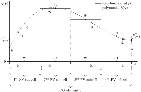
Figure 3: Schematic of four (N = 4) mean values and the reconstructed polynomial on the reference element. The cell boundary valuesu_q 1

2 andu⁺_q+1

2 were calculated with (37) where we assumed a blending factor of↵= 0.75.

where the outermost interface values are given by u_q 1

2 = (1 ↵q) (¯u1)q+↵qu˜_q and u⁺_q+1

2 = (1 ↵q) (¯uN)q+↵qu˜⁺_q. (37) A concrete example for the blended boundary valuesu^±_q±1

2 is shown in Fig. 3.

The common surface fluxf_q^⇤is then evaluated with the interface vectorsu⁺_q andu_q as

f_q^⇤=f^⇤ u⁺_q,u_q 2R^N+1. (38) To make the DG surface operatorBcompatible withf_q^⇤, we adapt the notation by inserting an additional column of zeros

B⁽⁰⁾= 0 BB

@

B11 0 · · · 0 · · · 0 B1N

B21 0 · · · 0 · · · 0 B2N

... ... ... ... ... ... ...

BN1 0 · · · 0 · · · 0 BN N

1 CC

A 2R^N⇥(N+1). (39)

Corollary:Contracting the DG surface operatorB⁽⁰⁾with the quadrature weights!is equivalent to the contraction of the FV surface operator, i.e.

!^TB⁽⁰⁾=1^{T (S)}. (40) Proof:We expand the left side of (40) and write

!^TB⁽⁰⁾ =

XN i=1

!i

`i( ¹₂)

!i

,0, . . . ,0, XN i=1

!i

`i(¹₂)

!i

!

=

XN i=1

`i( ¹₂),0, . . . ,0, XN i=1

`i(¹₂)

!

= ( 1,0, . . . ,0,1) =1^{T (S)}.

⇤ We replacefq^⇤(FV)andfq^⇤(DG) in (35) withf_q^⇤, and additionally, write the DG operators compactly, including the projection operator, as

Dˆ =P D and Bˆ =P B⁽⁰⁾. (41)

The final form of the single-level blended discretization is

@tu¯q= (1 ↵q) N

x f_q^⇤+↵q

1 x

⇣Dˆ f˜q B fˆ _q^⇤⌘

. (42)

Remark:It is easy to see that with↵q= 0for all elementsq, the pure subcell FV discretization is recovered and with

↵q= 1for all elements the blending scheme recovers the pure high order DG method.

Lemma:Given arbitrary blending factors↵q 2Rfor each elementqthe blending scheme (42) is conservative.

Proof:We discretely integrate the single-level blended discretization over all elementsqwith a total number ofQ XQ

q

xq1^T@tu¯q = XQ

q

xq1^Tn

(1 ↵q) N xq

f_q^⇤+↵q

1 xq

⇣Dˆf˜q B fˆ _q^⇤⌘ o . With (9) and (41) we get

XQ q

xq1^T@tu¯q = XQ

q

1^Tn

(1 ↵q)N ^(V)+ ^(S) f_q^⇤+↵q

⇣P Df˜q P B⁽⁰⁾f_q^⇤⌘ o . With properties (10), (24) and (26) the volume terms vanish, i.e.

1^{T (V)}=0^T and 1^TP D=N!^TD=0^T. We reformulate the DG surface term with (26) and (40) as

1^TP B⁽⁰⁾=N!^TB⁽⁰⁾=N1^{T (S)}. The expansion of the telescopic sum only leaves the outermost surface fluxes

XQ q

h (1 ↵q)N1^{T (S)} ↵qN1^{T (S)}i f_q^⇤=

XQ q

N1^{T (S)}f_q^⇤

= N⇣

f_{1 1}^⇤ + f_N+1^⇤ _Q⌘

= 0,

which represent the change due to physical boundary conditions. For instance in case of periodic boundary conditions,

these two fluxes would cancel to zero. ⇤

This concludes the description of the single-level blending scheme.

2.6 Multi-level Blending

As mentioned in the introduction, the general idea is the construction of ahierarchyof discretizations, with lower order DG schemes on sub-elements. In principle, it is thus possible to define a multi-level blending discretization, where the low order FV scheme is blended with DG variants of different approximation order. This multi-level extension is driven by the desire to retain as much ’high order DG accuracy’ as possible, especially on a sub-element level.

For the discussion, we consider a specific example setup with a DG element with polynomial degreeNp = 7. The data of this DG element is collected in form ofN = 8mean values on a regular subcell grid. Our goal is to blend a first order subcell FV scheme, a second and fourth order sub-element DG scheme and the full eight order DG scheme.

The construction of the individual schemes follows the discussion in the previous sections 2.1, 2.2, and 2.5. In this section, the extension to a multi-level blending approach is presented.

We get the first data interpretation and its corresponding discretization by directly using the mean values of elementq as a first order approximation space with no reconstruction at all

¯

u^O_q⁽¹⁾:=u¯q = (¯u1,u¯2, . . . ,u¯8)^T_q.

Next, we interpret the eight mean values as four second order DG sub-elements. The reconstruction matrixR^O(2) 2 R^2⇥2transforms two adjacent mean values to two nodal values

˜

u^O_q⁽²⁾=⇣

(˜u1)^O(2)₁ ,(˜u2)^O(2)₁

| {z }

O(2) sub-element

, . . . ,(˜u1)^O(2)₄ ,(˜u2)^O(2)₄

| {z }

O(2) sub-element

⌘T q =h

1₄⌦R^O(2)i

¯

uq. (43)

The fourth and eight order approximations are constructed analogously as

˜

u^O(4)_q =⇣

(˜u1)^O₁⁽⁴⁾, . . . ,(˜u4)^O₁⁽⁴⁾

| {z }

O(4) sub-element

,(˜u1)^O₂⁽⁴⁾, . . . ,(˜u4)^O₂⁽⁴⁾

| {z }

O(4) sub-element

⌘^T

q =h

1₂⌦R^O(4)i

¯

uq, (44) and

˜

u^O(8)_q =⇣

˜

u^O₁⁽⁸⁾, . . . ,u˜^O₈⁽⁸⁾

| {z }

O(8) sub-element

⌘^T

q =h

1₁⌦R^O(8)i

¯

uq, (45)

withR^O(4) 2 R^4⇥4 andR^O(8) 2 R^8⇥8. Here we used the Kronecker product⌦in conjunction with the identity matrix1_n =diag(1, . . . ,1)2 R^n⇥n in order to generate appropriate block-diagonal matrices. Fig. 18 in appendix 6.1 illustrates the hierarchy of the approximation spaces for this example.

We correspond the approximation spaces with the respective discretizations

@tu¯^O(1)_q = 8 xq

f^⇤

@tu¯^O_q⁽²⁾= 4 xq

⇢h1₄⌦Dˆ^O(2)i

f˜_q^O(2) h

1₄⌦Bˆ^O(2)i(0)

f_q^⇤ ,

@tu¯^O_q⁽⁴⁾= 2 xq

⇢h1₂⌦Dˆ^O(4)i

f˜_q^O(4) h

1₂⌦Bˆ^O(4)i(0)

f_q^⇤ , (46)

@tu¯^O(8)_q = 1 xq

⇢h1₁⌦Dˆ^O(8)i

f˜_q^O(8) h

1₁⌦Bˆ^O(8)i⁽⁰⁾ f_q^⇤ ,

where the DG volume fluxes are computed with the respective polynomial (sub-)element reconstructions of orders n={2,4,8}:

f˜_q^O(n)=f⇣

˜ u^O_q⁽ⁿ⁾⌘

. Similar to (39) the DG surface operators⇥1_N/n⌦Bˆ^O(n)⇤

had to be slightly adapted in order to be compatible with the common surface fluxf^⇤. We list the modified boundary evaluation matrices in the appendix 6.2. Finally, all four candidate discretizations are blended starting from the lowest order up to the highest order discretization

@tu¯⁰⁰⁰_q :=@tu¯^O_q⁽¹⁾,

,! @tu¯⁰⁰_q =⇣

1 ↵^O(2)_q ⌘

@tu¯⁰⁰⁰_q +↵^O(2)_q @tu¯^O(2)_q ,

,! @tu¯⁰_q=⇣

1 ↵^O_q⁽⁴⁾⌘

@tu¯⁰⁰_q +↵^O_q⁽⁴⁾ @tu¯^O_q⁽⁴⁾, (47) ,! @tu¯q=⇣

1 ↵^O_q⁽⁸⁾⌘

@tu¯⁰_q+↵^O_q⁽⁸⁾ @tu¯^O_q⁽⁸⁾,

where denotes the component-wise multiplication with the vector of blending parameters. Each DG sub-element computes its own blending factor according to the local data, i.e. we get 4 blending factors for theO(2)variant, 2 blending factors forO(4)and 1 forO(8)

↵^Oq⁽²⁾= ⇣

↵^O₁⁽²⁾,↵₂^O(2),↵^O₃⁽²⁾,↵^O₄⁽²⁾⌘^T

q ⌦ (1,1)^T,

↵^Oq⁽⁴⁾= ⇣

↵₁^O(4),↵^O₂⁽⁴⁾⌘T

q ⌦ (1,1,1,1)^T,

↵^Oq⁽⁸⁾= ↵^{O(8) T}_q ⌦ (1,1,1,1,1,1,1,1)^T. The actual strategy for the blending factors is described in the next section 2.7.

Again, as discussed in the case of a single-blending approach in section 2.5, special care is needed to preserve the conservation of the final discretization. Expanding on the idea in the single-level case, we aim to compute unique surface fluxes for each discretization with a uniquely defined interface value at sub-element or subcell interfaces. We

evaluate all high order DG polynomials at the FV subcell interfacesu^±Oq ⁽ⁿ⁾2R^N u^±O_q ⁽¹⁾:=u¯^O_q⁽¹⁾, u^±O_q ⁽²⁾=h

1₄⌦I^±O(2)i

˜ u^O_q⁽²⁾, u^±O_q ⁽⁴⁾=h

1₂⌦I^±O(4)i

˜

u^O_q⁽⁴⁾, u^±O_q ⁽⁸⁾=h

1₁⌦I^±O(8)i

˜ u^O_q⁽⁸⁾,

where the interpolation operatorI^±O(n) 2 R^n⇥n prolongates to the embedded FV subcell interfacesµ^O(n)_i±1/2 of the respective DG sub-element, i.e.

⇣I^±O(n)⌘

ij=`^O(n)_j ⇣ µ^O(n)_i±1/2⌘

, i, j= 1, . . . , n. (48) In Fig. 18 in appendix 6.1 two representatives ofµ^O_i±⁽ⁿ⁾_1/2 are shown which are aligned at the dotted vertical lines, indicating the interfaces of the FV subcells.

We start with the first order interpolation and stack on top the next levels of orders via convex blending u^±_q ⁰⁰⁰⁰ :=u^±O_q ⁽¹⁾

,! u^±_q ⁰⁰⁰=h

1 ↵^O_q⁽²⁾i

u^±_q ⁰⁰⁰⁰+↵^O_q⁽²⁾ u^±O_q ⁽²⁾

,! u^±_q ⁰⁰=h

1 ↵^O_q⁽⁴⁾i

u^±_q ⁰⁰⁰+↵^O_q⁽⁴⁾ u^±O_q ⁽⁴⁾

,! u^±_q ⁰ =h

1 ↵^O_q⁽⁸⁾i

u^±_q ⁰⁰+↵^O_q⁽⁸⁾ u^±O_q ⁽⁸⁾.

To arrive at a complete vector of interface values we append the element interface values from the left and right neighborsq 1andq+ 1.

u⁺_q =⇣ left neighbor

z }| { u⁺_N ⁰_{q 1},

internal boundaries

z }| { u⁺₁, . . . , u⁺_N ⁰_q⌘T

, u_q =⇣

u₁, . . . , u_N ⁰_q,

| {z }

internal boundaries

u₁ ⁰_q+1

| {z }

right neighbor

⌘T

.

These new common interface values allow us to evaluate a common surface flux (38) at each interface, which is again the key to preserve conservation in the final discretization. This concludes the description of the multi-level blending scheme.

2.7 Calculation of the Blending Factor↵

A good shock indicator for high order methods is supposed to recognize discontinuities, such as weak and strong shocks, in the solution early on and mark the affected elements for proper shock capturing. On the other hand, the indicator should avoid to flag non-shock related fluid features such as shear layers and turbulent flows. There are numerous indicators available for DG schemes [50, 15, 14, 60, 2, 9, 66].

In this work we want to construct an a-priori indicator which relies on the readily available information within each element provided by the multi-level blending framework introduced in section 2.6. The principal idea is to compare a measure of smoothness of the different order reconstructions with each other. Smooth, well-resolved flows are expected to yield rather similar solution profiles compared to data that contain strong variations.

The smoothness measure q^O(n)within elementqof then-th order reconstructionu˜^Oq⁽ⁿ⁾is inferred from theL¹-norm of its first derivative. For example, if we want to calculate the blending factor↵^Oq⁽⁸⁾for the eighth order we compute

O(8)

q =

Z ¹₂

1 2

@⇠u˜^O_q⁽⁸⁾(⇠) d⇠ (49)

and

O(4)

q =⇣ _O(4)

1

⌘

q+⇣ _O(4)

2

⌘

q = Z 0

1 2

@⇠

⇣u˜^O(4)₁ ⌘

q(⇠) d⇠+ Z ¹₂

0

@⇠

⇣u˜^O(4)₂ ⌘

q(⇠) d⇠

utilizing information from the top-level eighth order element and its two fourth order sub-elements. The integrals are evaluated with appropriate quadrature rules. Then the blending factor is calculated by comparing the smoothness of the different orders as

↵^O(8)_q = 1 cutoff 0

@0,⌧A

0

@

O(8)

q O(4)

q

max q^O(4), ^Oq⁽⁸⁾,1 ⌧S

1 A,1

1

A, (50)

where cutoff(xlower, x, xupper) = min(max(xlower, x), xupper) and with two parameters ⌧A,⌧S > 0. The design of equation (50) ensures that↵^Oq⁽ⁿ⁾is always within the unit interval and that for very small q^O(n)the indicator does not get hypersensitive due to floating point truncation. If not noted otherwise we set the amplification parameter to

⌧A = 100and the sensitivity parameter⌧S = 0.05. The latter parameter has the biggest influence on the behavior of the indicator and its value demarcates the lower bound where it does not interfere with the convergence tests conducted in section 3. In order to capture all troubling flow features we independently apply the indicator (50) on all primitive state variables and select the smallest of the resulting blending factors. The calculations of the two fourth order blending factors⇣

↵^O(4)₁ ⌘

q and⇣

↵^O(4)₂ ⌘

q are done within each sub-element independently together with their respective second order smoothness measures⇣ _O(2)

s

⌘

q,s= 1, . . . ,4.

For piecewise linear polynomials, the indicator (50) is not applicable. Instead, we directly use the squeezing parameter obtained from the positivity limiter in (30), i.e.↵^Os⁽²⁾ := s^O(2),s= 1, . . . ,4.

Remark:The indicator (50) is also used for the single-level blending scheme.

2.8 Sketch of the Algorithm

In the last part of this section, a sketch of the algorithm for the blending framework is presented. We present a general outline of the necessary steps for the 1D single-blending scheme evolved with a multi-stage Runge-Kutta time stepping method. We enter at the beginning of a Runge-Kutta cycle and do the following.

(I) Reconstruct the polynomialu˜qfrom the given mean valuesu¯qfor each elementqas in (28).

(II) If the reconstructed polynomialu˜q contains non-permissible states, see (31), then calculate the limited version

˜

u^{( )}q as in (30)

(III) If the squeezing parameter q is below Lthen set↵q := 0else compute the blending factor↵q via (50) from theunlimitedpolynomialu˜q.

(IV) Compute the boundary values u^±_q via (37) and exchange alongside zone boundaries in case of distributed computing.

(V) Determine the common surface fluxf_q^⇤via (38).

(VI) Calculate the right-hand-side@tu¯q:

. If the blending factor↵qabove↵Hthen compute@tu¯q with the DG-only scheme.

. Else if the blending factor↵qbelow↵Lthen compute@tu¯qwith the FV-only scheme.

. Else compute@tu¯qwith the single-level blending scheme (42).

(VII) Forward in time to the next Runge-Kutta stage and return to step (I).

The switching thresholds are set to↵H := 0.99and↵L:= 0.01and the limiter threshold to L:= 0.95. Note that the algorithm only applies the blending procedure where necessary in order to maintain the overall performance of the scheme.

This concludes the presentation of the 1D blending scheme. The description of the blending scheme on 3D Cartesian meshes as well as the algorithm outline for the multi-level blending scheme can be found in appendix 6.3 and 6.4.

3 Validation

For the computational investigations, the multi-level algorithm with the explicit SSP-RK(5,4) time integrator [59]

is implemented in a Fortran-2008 prototype code with a hybrid parallelization strategy based on MPI and OpenMP.

Management of the AMR and load balancing is provided by^P4^EST, a highly efficient Octree library [4]. The maximal time step for dimensionsd= 1,2,3is estimated by the CFL condition

t:=CF Lmin

q

xq

2^{d 1}(2N 1) ¯q,max, (51)

whereCF L:= 0.8,N := 8is the number of mean values in each direction of the elementqand¯_q,maxis an estimate of the maximum eigenvalue given in (55). For the numerical interface fluxesf^⇤, we use the Harten-Lax-Leer (HLL) approximate Riemann solver [29] with Einfeldt signal speed estimates [16].

3.1 Governing Equations

We consider the compressible Euler equations

@t⇢+r·(⇢v) = 0,

@t(⇢v) +r· ⇢vv^T +p1 =0, (52)

@tE+r·⇣

v(E+p)⌘

= 0,

with the vector of conserved quantitiesu= (⇢,⇢v,E)^T, where⇢denotes the density,vthe velocity, andEthe total energy. We assume a perfect gas equation of state and compute the pressure as

p(u) = ( 1)h

E ⇢

2v^Tvi

. (53)

If not stated otherwise we choose = 1.4. The set of permissible states is given by

permissible states = 8u ⇢>0^p(u)>0 . (54) For the CFL condition (51) the maximum eigenvalue is evaluated on all mean valuesu¯qof elementq. Given dimension d={1,2,3}it reads as

¯_q,max= max

i,d

✓

(¯vd)i + r p¯i

¯

⇢i

◆

, i= 1, . . . , N^dmax. (55)

3.2 Convergence Test

We use the manufactured solution method [52] and validate the 3D multi-level blending scheme on a periodic cube of unit length (L= 1) where the resolution of the mesh is incrementally doubled. We define our manufactured solution in primitive state variables as

⇢(t;x, y, z) = 1.0 + 0.35 sin

✓2⇡(x t) L

◆

+ 0.24 cos

✓2⇡(y t) L

◆

+ 0.1 sin

✓2⇡(z t) L

◆ ,

v(t;x, y, z) = (0.1,0.2,0.3)^T, (56)

p(t;x, y, z) = 1.0 + 0.23 cos

✓2⇡(x t) L

◆

+ 0.19 sin

✓2⇡(y t) L

◆

+ 0.2 cos

✓2⇡(z t) L

◆ .

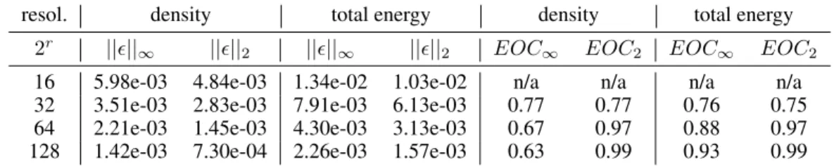
The final time of the simulation is T = 2 and the center of the domain is refined to introduce non-conforming interfaces in the computational domain. We determine theL¹- andL²-norms of the errors in the density and total energy. Tables 1 to 4 list the results for the first, second, fourth and eighth order multi-level blending schemes. The initial conditions and the source term of our manufactured solution (56) is in all cases evaluated and applied on the mean values via an appropriate quadrature rule to maintain high order. The results confirm, that the discretizations behave as designed in this assessment.

Table 1: Experimental order of convergence of the first-order FV variant within the 3D multi- level blending framework.

resol. density total energy density total energy

2^r ||✏||1 ||✏||² ||✏||1 ||✏||² EOC₁ EOC2 EOC₁ EOC2

16 5.98e-03 4.84e-03 1.34e-02 1.03e-02 n/a n/a n/a n/a

32 3.51e-03 2.83e-03 7.91e-03 6.13e-03 0.77 0.77 0.76 0.75 64 2.21e-03 1.45e-03 4.30e-03 3.13e-03 0.67 0.97 0.88 0.97 128 1.42e-03 7.30e-04 2.26e-03 1.57e-03 0.63 0.99 0.93 0.99 Table 2: Experimental order of convergence of the second order DG variant within the 3D multi-level blending framework.

resol. density total energy density total energy

2^r ||✏||1 ||✏||² ||✏||1 ||✏||² EOC₁ EOC2 EOC₁ EOC2

16 1.46e-03 5.38e-04 2.21e-03 9.35e-04 n/a n/a n/a n/a

32 4.59e-04 9.29e-05 6.63e-04 1.97e-04 1.67 2.53 1.74 2.25 64 1.11e-04 1.77e-05 1.48e-04 4.26e-05 2.04 2.39 2.17 2.21 128 2.63e-05 3.88e-06 3.09e-05 9.72e-06 2.08 2.19 2.25 2.13 Table 3: Experimental order of convergence of the fourth order DG variant within the 3D multi-level blending framework.

resol. density total energy density total energy

2^r ||✏||1 ||✏||² ||✏||1 ||✏||² EOC₁ EOC2 EOC₁ EOC2

16 1.10e-04 6.45e-05 3.20e-04 1.83e-04 n/a n/a n/a n/a

32 7.86e-06 4.33e-06 2.19e-05 1.33e-05 3.80 3.90 3.87 3.79 64 5.18e-07 2.59e-07 1.31e-06 7.59e-07 3.92 4.07 4.07 4.13 128 3.45e-08 1.82e-08 7.75e-08 4.29e-08 3.91 3.83 4.07 4.15 Table 4: Experimental order of convergence of the eighth order DG variant within the 3D multi-level blending framework. Here we setCF L:= 0.1, as the time integration method is only fourth order accurate.

resol. density total energy density total energy

2^r ||✏||1 ||✏||² ||✏||1 ||✏||² EOC₁ EOC2 EOC₁ EOC2

16 2.77e-07 1.65e-07 7.77e-07 4.55e-07 n/a n/a n/a n/a

32 2.77e-09 1.00e-09 6.72e-09 2.41e-09 6.65 7.36 6.85 7.56 64 1.73e-11 3.48e-12 4.15e-11 1.04e-11 7.32 8.17 7.34 7.86 128 8.06e-14 1.87e-14 1.85e-13 6.74e-14 7.74 7.54 7.81 7.27

3.3 Conservation Test

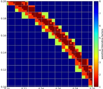
The goal in this assessment is to demonstrate that the multi-level-blending discretization is conservative for all choices of blending factors. To do so, we adapt the same setup as in section 3.2 but deactivate the source term. The center of the domain is refined to introduce non-conforming interfaces in the computational domain. Additionally, as a stress test, the blending factors are randomly chosen and changed after each Runge-Kutta stage. As there are multiple blending factors at a given spatial location, we consider the following weighted blending factor

¯

↵=nh⇣

1 ↵^O(2)⌘

+ 2↵^O(2)i ⇣

1 ↵^O(4)⌘

+ 4↵^O(4)o ⇣

1 ↵^O(8)⌘

+ 8↵^O(8), (57) to illustrate the distribution of the blending factors in Fig.4. Note the limiting cases↵¯ = 1for pure FV and↵¯= 8for the eighth order DG scheme.

The simulation runs toT = 300performing more than a quarter million timesteps. The result of the test is shown in Fig. 5 where we plot in log-scale the absolute value of thechange of bulk@t¯_total(t), integrated over the whole domain,

@t¯_total(t) = XQ

q

1

|⌦q| Z

⌦q

@t¯(t)d⌦. (58)

Qis the total number of elements and|⌦q| = xq yq zq is the volume per element. The results show that the conservation error lies within the range of 64 bit (double precision) floating point truncation and hence confirm that the multi-level blending discretization is fully conservative up to machine precision errors.

Figure 4: Conservation test of the 3D multi-level blending scheme: Slice through the computational domain showing weighted blending factor↵¯according to (57) on a Cartesian non-conforming mesh with refinement levels 3 to 5. The black lines depict the boundaries of the corresponding 8th order DG elements.

Figure 5: Conservation test of the 3D multi-level blending scheme: Evolution of the integrated change of bulk log₁₀(|@t¯_total|)(eq. (58)) of each conservative state variable.