The Discontinuous Galerkin method

(1)

The Discontinuous Galerkin method

Heiner Igel

Department of Earth and Environmental Sciences Ludwig-Maximilians-University Munich

1

(2)

Outline

Introduction Motivation History

The Discontinuous Galerkin Method in a Nutshell Ingredients

Solution to Scalar Advection Equation

The Discontinuous Galerkin Method Put To Action

(3)

Introduction

(4)

Motivation

• Efficiently solving the elastic wave equation on tetrahedral grids

• Easy implementation of local time stepping

• High accuracy of frictional boundary

conditions for dynamic rupture problems

(5)

History

• Developed in the Los Alamos National Laboratories for the problem of neutron transport by Reed 1973 formulated on triangular meshes

• In the late eighties Cockburn connected discontinuous Galerkin method with high-order Runge-Kutta-type time integration schemes (Cockburn et al., 2000)

• First application to elastic wave propagation was published by Kaeser and Dumbser, 2006

• Kaeser et al., 2008 carried out a detailed analysis of the convergence properties of the discontinuous Galerkin method

• The local time-stepping approach by Dumbser et al., 2007b circumvents the problem of oversampling large parts of the model and thereby reducing the overall computations.

• De la Puente et al., 2009b reported a first analysis of scaling and synchronization of the discontinuous Galerkin method which raised the interest of the computational science community in Munich to optimize it.

4

(6)

History

(7)

History

4

(8)

History

(9)

History

4

(10)

History

(11)

The Discontinuous Galerkin Method in a Nutshell

All concepts that have been discussed previously enter in this method 1 Finite-difference extrapolation using e.g. the Euler scheme 2 Calculation of element-based stiffness and mass matrices

3 Flux calculations at the element boundaries as encountered in the finite-volume method

4 Exact nodal interpolation based on Lagrange polynomials 5 Numerical integration schemes using collocation points

5

(12)

Wave Equation

1st order wave equation

ρ∂

_t

v = ∂

_x

σ + f

∂

_t

σ = µ∂

_x

v Matrix-vector form

∂

t

Q + A∂

x

Q = f

(13)

Wave Equation

where σ = σ

xy

= σ

yx

representing the only non-zero stress component, and implicitly assuming space-time dependencies, Q = (v , σ) is the vector of unknowns and A contains the coefficients of the equation given by

A = 0 −1/ρ

−µ 0

! .

= ⇒ Linear hyperbolic system, having the same form as the classic advection equation

7

(14)

The Discontinuous Galerkin Method in a Nutshell

• The Ansatz is to multiply the equation by an arbitrary test function combined with describing the unknown fields with the same set of basis functions (Galerkin principle).

• At the element boundaries the unknown fields can be discontinuous.

• Communication between the elements is achieved through a flux scheme

based on solutions of the Riemann problem.

(15)

The Discontinuous Galerkin Method in a Nutshell

The wavefield inside each element is described by La- grange polynomials exactly interpolating at appropriate collocation points. At each time step, a flux term F has to be evaluated at all element boundaries. The extrapolation scheme of the discontinuous Galerkin method can be expressed as

∂

t

Q

^k

(t) = (M

^k

)

⁻¹

(K

^k

Q

^k

(t) − (F

_l^k

− F

_r^k

)Q

^k

(t)) where Q(t) is the vector of unknowns, M and K are the elemental mass and stiffness matrices, respectively, and F

r,l

are the flux terms at the left and right boundaries. The upper index k denotes the element (source term is omitted).

9

(16)

The Discontinuous Galerkin Method in a Nutshell

Implications of a boundary flux and no global system of equations to solve:

1 Obtaining a fully explicit scheme which lends itself to an element-based parallelization scheme

2 Choice of element size is arbitrary, it has no impact on the solution algorithm (h-adaptivity)

3 The polynomial order in each element can be arbitrarily chosen and no impact on the algorithm (p-adaptivity)

4 Considering the boundary points twice to calculate the fluxes implies an

increase in the number of degrees of freedom that of course gets worse

with increasing dimensionality

(17)

Ingredients

(18)

Source-free version of the coupled elastic wave equation in 1D

∂

t

σ − µ∂

x

v = 0

∂

t

v − 1

ρ ∂

x

σ = 0 Matrix notation

∂

t

Q + A∂

_x

Q = 0

where Q = (σ, v ) is the vector of unknowns and matrix A contains the parameters A = 0 −µ

−

¹_ρ

0 !

(19)

The Wave equation as Hyperbolic System

In the case of a quadratic matrix A with shape m × m, this leads to an eigenvalue problem. If we were able to obtain eigenvalues λ

p

such that

Ax

_p

= λ

p

x

_p

, p = 1, ..., m we get a diagonal matrix of eigenvalues

Λ =





 λ

₁

. ..

λ

_m







and the corresponding matrix R containing the eigenvectors x

_p

in each column R = (x

₁

|x

₂

| . . . |x

_p

)

12

(20)

The Wave equation as Hyperbolic System

The Jacobian matrix A can now be expressed with the definitions A = RΛR

⁻¹

Λ = R

⁻¹

AR . Applying these definitions to the wave equation

R

⁻¹

∂

t

Q + R

⁻¹

RΛR

⁻¹

∂

x

Q = 0 and introducing the solution vector W = R

⁻¹

Q results in

∂

t

W + Λ∂

x

W = 0 .

(21)

The Wave equation as Hyperbolic System With λ

_1,2

= p

µ/ρ = ±c, where c corresponds to the shear velocity, the eigenvectors can be obtained

r

_1,2

= ±ρc 1

!

interestingly enough containing as elements values of the seismic impedance Z = ρc that are relevant for the reflection behaviour of seismic waves. Thus the matrix R (and its inverse) are

R = Z −Z

1 1

!

, R

⁻¹

= 1 2Z

1 Z

−1 Z

! .

14

(22)

The Wave equation as Hyperbolic System

The wave equation in the rotated eigensystem can be stated as

∂

_t

w

₁

w

₂

!

+ −c 0

0 c

!

∂

_x

w

₁

w

₂

!

= 0

with the simple general solution w

_1,2

= w

_1,2⁽⁰⁾

(x ± ct), where the upper index 0 stands for the initial condition (i.e., waveform that is advected). The initial condition also fullfills W

⁽⁰⁾

= R

⁻¹

Q

⁽⁰⁾

, we can therefore relate the so-called characteristic variables w

_1,2

to the initial conditions of the physical variables as

w

₁

(x , t) = 1

2Z (σ

⁽⁰⁾

(x + ct) + Zv

⁽⁰⁾

(x + ct )) w

₂

(x , t) = 1

2Z (−σ

⁽⁰⁾

(x − ct ) + Zv

⁽⁰⁾

(x − ct))

(23)

The Wave equation as Hyperbolic System

To obtain the final analytical solution for velocity v and stress σ using Q = RW as σ(x , t) = 1

2 (σ

⁽⁰⁾

(x + ct ) + σ

⁽⁰⁾

(x − ct )) + Z

2 (v

⁽⁰⁾

(x + ct ) − v

⁽⁰⁾

(x − ct)) v (x , t) = 1

2Z (σ

⁽⁰⁾

(x + ct) − σ

⁽⁰⁾

(x − ct )) + 1

2 (v

⁽⁰⁾

(x + ct ) + v

⁽⁰⁾

(x − ct)) . In compact form, the solution can be expressed as

Q(x , t) =

m

X

p=1

w

p

(x, t)r

p

16

(24)

Solution to Scalar Advection Equation

Denoting q (x , t) for the unknown scalar solution and a for the given (possibly space dependent) advection (wave) velocity to obtain the source-free wave equation

∂

_t

q(x , t ) + a ∂

_x

q(x , t) = 0

The physical domain of each element is denoted by D

_k

with left and right boundaries x

_l^k

and x

_r^k

, respectively. Note the varying element sizes (h-adaptivity).

(25)

Solution to Scalar Advection Equation

The k elements are non-overlapping which implies a higher number of degrees of freedom. The solution vector in 1D is

q

_N_p

=







q

₁¹

q

₁²

. . . q

ⁿ₁

q

₂¹

q

₂²

. . . q

ⁿ₂

.. . .. . . .. .. . q

_N¹_p

q

_N²_p

. . . q

ⁿ_N_p







where N

_p

is the number of points per element and n the overall number of elements. The collocation points are Gauss-Lobatto-Legendre stored as

x

Np

=







x

₁¹

x

₁²

= x

_N¹_p

. . . x

₁ⁿ

x

₂¹

x

₂²

. . . x

₂ⁿ

.. . .. . . .. .. . x

_N¹_p

= x

₁²

x

_N²_p

. . . x

_Nⁿ_p





 .

18

(26)

Solution to Scalar Advection Equation

The global solution requires the adoption of flux concepts. Therefore a special sign is introduced that links the element-level to the global solution as

q(x , t) ≈ q

_h

(x , t) =

n

M

k=1

q

_h^k

(x , t) where L

indicates global assembly, n is the overall number of elements and h is

the size of element k .

(27)

Weak formulation

To obtain the weak formulation of the scalar advection equation we multiply it

∂

_t

q(x , t) + a ∂

_x

q(x , t) = 0

with a general test function φ

_j

(x ), integrate over the k-th element domain D

_k

to

obtain Z

Dk

∂

t

q(x , t)φ

_j

(x )dx + Z

Dk

a∂

x

q(x , t)φ

_j

(x )dx = 0

20

(28)

Weak formulation

And partially integrate replacing the term containing the space derivative by Z

D_k

a∂

_x

q(x , t)φ

_j

(x)dx = [aq(x , t)φ

_j

(x )]

^x_x^r_l

− Z

Dk

aq(x , t)∂

x

φ

_j

(x )dx

where x

r

and x

_l

are the right and left boundaries of element k , and we assume

constant velocity a inside the element.

(29)

Weak formulation

What does the rule of partial integration look like with more than one dimension? The definition is known as

Z

Ω

∂

x_i

uvd Ω = Z

Γ

uvn

_i

d Γ

− Z

Ω

u∂

_x_i

vd Ω

where u, v are arbitrary space-dependent functions, Ω denotes the entire volume, Γ its boundary, and n

_i

is a vector normal to the boundary.

22

(30)

Weak formulation

Putting this into the advection equation we obtain for element k Z

D_k

∂

_t

q(x , t)φ

_j

(x )dx − Z

D_k

aq(x , t)∂

_x

φ

_j

(x)dx

= − [aq(x , t)φ

_j

(x )]

^x_x^r_l

Replacing the unknown field q(x, t) by a finite polynomial representation in terms

of a weighted sum over Lagrange polynomials inside each element k of order N

denoted as `

_i

(x), i = 1, . . . , N + 1 defined in the interval x ∈ [−1, 1].

(31)

Weak formulation

With the exact interpolation property of the Lagrange polynomials at the Gauss-Legendre-Lobatto collocation points x

_i

, here illustrated for an arbitrary function y

_i

= y (x

_i

)

y

_i

=

Np

X

j=1

y

_j

`

_j

(x

_i

) =

Np

X

j=1

y

_j

δ

_ij

we obtain for element k

q(x , t)|

_x=x_i

=

Np

X

i=1

q

_i

(t) `

i

(x )

where N

p

indicates that in each element the polynomial order may vary, x = x

_i

are the collocation points.

24

(32)

Weak formulation

In addition we also replace the test function by Lagrange polynomials. Combining this we yield

Z

D_k

∂

t Np

X

i=1

q

_i

(t)`

_i

(x)`

_j

(x )dx − Z

D_k

a

Np

X

i=1

q

_i

(t)`

_i

(x)∂

_x

`

_j

(x )dx and after re-ordering (omitting space dependencies of polynomials)

Np

X

i=1

Z

D_k

`

i

(x )`

j

(x )dx

∂

t

q

_i

(t) − Z

D_k

a`

_i

(x )∂

x

`

j

(x )dx

q

_i

(t)

(33)

Weak formulation

Recognizing the elemental mass M

ij

and stiffness K

ij

matrices in this equation. Assuming implicit matrix-vector operations we obtain

M ∂

_t

q (t ) − K

^T

q(t) where the matrices are given by

M

ij

= Z

Dk

`

_i

(x )`

_j

(x)dx K

_ij

=

Z

Dk

a`

_i

(x )∂

_x

`

_j

(x )dx

assuming constant velocity a inside element k . Note that the lower index D

k

indicates that we are still in physical space and we have to map to the local coordinate system.

26

(34)

Elemental Mass and Stiffness Matrices

The matrices (nodal or modal approach) for arbitrary test functions φ

_i

(x ) are defined by

M

_ij

= Z

Dk

φ

_i

(x )φ

_j

(x ) dx K

_ij

= a

Z

D_k

φ

i

(x )∂

x

φ

j

(x ) dx

containing integrals over (derivatives of) the test functions φ(x ). Replacing the integrals by a weighted sum over the function values f (x

_i

) at carefully chosen points x

_i

inside the elements

Z

Ω

f (x ) dx ≈

N

X

i=1

w

_i

f (x

_i

)

(35)

Elemental Mass and Stiffness Matrices

We need to map our physical coordinates into an element-based system. In 1D this is quite simple using as local variable ξ and transforming via

x

^k

(ξ) = x

_l^k

+ (1 + ξ)

2 dx ξ ∈ [−1, 1]

where x

_l^k

and x

_r^k

are the left and right physical boundaries of element k . In general the mapping of the differential used to evaluate integrals is called the Jacobian defined for element k as

J

^k

= dx

d ξ , J

^k

= x

_r^k

− x

_l^k

1 − (−1) = h

^k

2 where h

^k

is the size of element k .

28

(36)

Elemental Mass and Stiffness Matrices

For the elemental matrices we obtain for general test functions M

_ij

=

Z

Dk

φ

_i

(ξ)φ

_j

(ξ)J

^k

d ξ K

_ij

= a

Z

D_k

φ

_i

(ξ)∂

_ξ

((J

^k

)

⁻¹

)J

^k

φ

_j

(ξ) d ξ

= a Z

D_k

φ

_i

(ξ)∂

_ξ

φ

_j

(ξ)d ξ

(37)

Elemental Mass and Stiffness Matrices

Finally, we can replace the test function with the Lagrange polynomials of order N

_p

leading to the definition of the mass and stiffness matrices

M

_ij

= Z

1

−1

`

_i

(ξ)`

_j

(ξ) J

^k

d ξ =

Np

X

m=1

w

_m

`

_i

(x

_m

)`

_j

(x

_m

) J

^k

=

Np

X

m=1

w

_m

δ

im

δ

jm

J

^k

=







w

_i

J

^k

if i = j 0 if i 6= j

30

(38)

Elemental Mass and Stiffness Matrices

K

_ij

= Z

1

−1

`

_i

(ξ)∂

_x

`

_j

(ξ) d ξ =

Np

X

m=1

a w

_m

`

_i

(x

_m

)∂

_x

`

_j

(x

_m

)

=

Np

X

m=1

a w

m

δ

_im

∂

x

`

_j

(x

m

)

=a w

_i

∂

x

`

_j

(x

_i

) .

(39)

The Flux Scheme

The key task in the discontinuous Galerkin scheme concerns the question what values to allocate to the points at the element boundaries. This involves the use of flux schemes.

32

(40)

The Flux Scheme

Starting with the r.h.s. of this equation Z

Dk

∂

_t

q(x , t)φ

_j

(x )dx − Z

Dk

aq(x , t)∂

_x

φ

_j

(x)dx

= − [aq(x , t)φ

_j

(x )]

^x_x^r_l

The originial form holds also for higher dimensions

Z

∂D_k

a q(x, t)φ

_j

(x ) n dx

where n = ±1 denotes the vector normal to the boundary, in 1D taking the values

n = −1 and n = 1 at the left and right boundaries.

(41)

The Flux Scheme

Replacing the space-dependent part of q(x , t ) by a sum over Lagrange polynomials to obtain

Np

X

i=1

Z

∂Dk

`

_j

(x ) `

_i

(x) a q

i

(t ) n dx

and also replacing the arbitrary test function with the same function. The orthogonality of the Lagrange polynomials and the fact that we are integrating over the surface ∂D

_k

leads to

Np

X

i=1

(`

_i

(x

_r^k

) `

_j

(x

_r^k

)(a q(x

_r^k

))

^∗

− `

_i

(x

_l^k

) `

_j

(x

_l^k

)(a q(x

_l^k

))

^∗

)

= `

_j

(x

_r^k

)(a q(x

_r^k

))

^∗

− `

_j

(x

_l^k

)(a q(x

_l^k

))

^∗

where we introduced the starred terms (a q(x

_r,l^k

))

^∗

that are the values at the element boundaries.

34

(42)

The Flux Scheme

Therefore, we introduce the general flux vector with elements F

_j

(a, q

^k

(x , t)), j = 1, .., N

_p

as

F

_j

(a, q

^k

(x , t)) = [`

_j

(x ) (a q(x , t))

^∗

]

^x_x^r^kk l

In vector form

F =





 F

₁

0 .. . 0 F

_N_p







=







−(a q(x , t))

^∗

(x

_l^k

) 0

.. . 0 (a q(x, t))

^∗

(x

_r^k

)







.

(43)

The Flux Scheme

At the left boundary the outside value in element k − 1 is denoted with "‘+"’ and the value inside element k with "‘-"’. The starred value q ∗ (x

_l^k

) is the flux that needs to be defined as a function of the boundary values of the adjacent elements.

36

(44)

The Flux Scheme

Taking the average of the values from both sides of the boundaries - also called the central flux - can be expressed as

F

₁^c

= 1

2 a

^k

(q(x

_r^k⁻¹

, t) + q(x

_l^k

, t)) F

_N^c_p

= 1

2 a

^k

(q(x

_r^k

, t) + q(x

_l^k+1

, t)) The simplemost, stable choice is the so called upwind flux

F

₁^up

=







a

^k

q(x

_l^k

) if a

^k

≤ 0 a

^k⁻¹

q(x

_r^k⁻¹

) if a

^k−1

> 0 F

_N^up

p

=







a

^k⁺¹

q(x

_l^k⁺¹

) if a

^k⁺¹

≤ 0

a

^k

q(x

_r^k

) if a

^k

> 0

(45)

The Flux Scheme

Centered and upwind fluxes can be formulated in a compact way. This formulation reads

F

₁

= −a 1

2 (q(x

_l^k

) + q(x

_r^k−1

)) − |a|

2 (1 − α)(q(x

_r^k⁻¹

) − q(x

_l^k

)) F

_N_p

= a 1

2 (q(x

_r^k

) + q(x

_l^k+1

)) + |a|

2 (1 − α)(q(x

_r^k

) − q(x

_l^k+1

)) where α = 0 corresponds to the upwind flux and α = 1 to the centered flux scheme.

38

(46)

The Discontinuous Galerkin

Method Put To Action

(47)

The Discontinuous Galerkin Method Put To Action

In matrix notation we yielded for one element

M∂

_t

q(t) − K

^T

q(t) = −F (a, q(t)) requiring an extrapolation scheme of the form

∂

_t

q(t) = M

⁻¹

(K

^T

q(t) − F (a, q(t)))

where F (a, q(t)) is the flux vector as defined above. We seek to extrapolate the system from some initial conditions and obtain using the simple Euler method for each element

q(t

_n+1

) ≈ q(t

n

) + dt h

M

⁻¹

(K

^T

q(t

n

) − F (a, q(t)) i

where for the flux scheme F() we use the upwind approach.

₃₉

(48)

The Discontinuous Galerkin Method Put To Action

Employing a high-order extrapolation procedure known as predictor-corrector method (or Heun’s method, or two-stage Runge-Kutta method). At time step t

_i

using time increment dt

k

₁

= f (t

_i

, y

_i

)

k

₂

= f (t

_i

+ dt , y

_i

+ dtk

₁

) y

_i+1

= y

_i

+ 1

2 dt(k

₁

+ k

₂

)

(49)

The Discontinuous Galerkin Method Put To Action

The matrix-vector form of the discontinuous Galerkin method. The system of questions at an elemental level is illustrated by plotting the absolute matrix/vector values. N = 3, N

_p

= N + 1 = 4

41

(50)

The Discontinuous Galerkin Method Put To Action

% Initialize vectors, matrices Minv = zeros(N+1,N+1,ne);

K = zeros(N+1,N+1,ne);

q = zeros(N+1,ne);

(...) for k=1:ne, for i=1:N+1,

Minv(i,i,k)=1./(w(i)*J(k);

end end (...) for k=1:ne, for i=1:N+1, for j=1:N+1,

K(i,j,k)=a(k)*w(i)*l1d(j,i);

end end

The most important initialization step is the

calculation of the elemental matrices, mass

M and stiffness K . The following code part

illustrates a possible implementation looping

through all elements ne and calculating these

matrices as a function of the Jacobian J(k ) =

h

^k

/2 where h

^k

is the size of element k :

(51)

The Discontinuous Galerkin Method Put To Action

% Flux calculation F = zeros(N+1,ne);

(...) for k=1:ne,

F(1,k)= -a*(q(1,k)+q(N+1,k-1))/2 - abs(a)*(1-alpha)/2*(q(N+1,k-1)-q(1,k));

F(N+1,k)= a*(q(N+1,k)+q(1,k+1))/2 + abs(a)*(1-alpha)/2*(q(N+1,k)-q(1,k+1));

end

The flux vector has to be calculated new for each time step (or intermediate step when using high-order extrapolation schemes) as it depends on the current values of the wavefield q. alpha can be used to change the flux scheme from central (alpha = 1) to upwind (alpha = 0).

43

(52)

The Discontinuous Galerkin Method Put To Action

The element-wise system of equations can be extrapolated by the Euler scheme as

% Time extrapolation for it = 1:nt,

(...)

% Initialize flux vectors F (...) for k=1:ne,

q(:,k) = q(:,k) + dt .* (Minv(:,k) * (K(:,k)’*q(:,k)-F(:,k)));

end (...) end

where nt is the overall number of time steps, dt is the global time increment, and

ne is the number of elements. Note that can directly update the solution vector q

without intermediate storage at different time level(s).

(53)

The Discontinuous Galerkin Method Put To Action

A high-order extrapolation scheme like the predictor-corrector method can be implemented as

% Time extrapolation for it = 1:nt,

(...)

% Predictor corrector scheme

% Initialize flux vectors F for all k (...)

% First step (predictor) for i=1:k,

k1(:,k)= Minv(:,k) * (K(:,k)’*q(:,k)-F(:,k));

end (...)

% Initialize flux vectors F for q+dt*k1 (...)

% Second step (corrector) for i=1:k,

k2(:,k)= Minv(:,k) * (K(:,k)’*(q(:,k)+dt*k1(:,k))- F(:,k));

end (...)

% Update for i=1:k,

q(:,k)= q(:,k) + dt (k1(:,k) + k2(:,k));

end (...) end

45

(54)

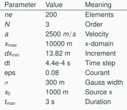
Example

Table 1: Simulation parameters for 1D discontinuous Galerkin advection Parameter Value Meaning

ne 200 Elements

N 3 Order

a 2500 m/s Velocity

x

max

10000 m x-domain

dx

min

13.82 m Increment

dt 4.4e-4 s Time step

eps 0.08 Courant

σ 300 m Gauss width

x

0

1000 m Source x

t

max

3 s Duration

−1/σ²(x−x )²

(55)

Example

47

(56)

Summary

• The discontinuous Galerkin method is a finite-element type method. The main difference is that the solution fields are not continuous at the element boundaries.

• The elemental mass and stiffness matrices are formulated very similar to the classic finite-element schemes. However, they are never assemble to a global system of equations. Therefore no large system matrix needs to be inverted.

• Elements are linked by a flux scheme, similar to the finite volume method. This scheme leads to an entirely local algorithm in the sense that all calculations are carried out at an elemental level. Communication happens only to direct neighbours.

• The discontinuous Galerkin scheme can easily to higher orders, keeping the local nature of the solution scheme. This leads to high efficiency when parallelizing the scheme.

(57)

Summary

• The solution fields can be extended using nodal and modal approaches. Modal approaches are preferred for tetrahedral schemes. Nodal solutions are preferred for hexahedral meshes.

• The discontinuous behaviour at the element boundaries and the associated discretization of the element boundaries increases the number of degrees of freedom compared to other methods.

• The flexibility with polynomial order, element size, local time stepping leads to a formidable problem when parallelizing a discontinuous Galerkin method: load balancing the computational task is not easy! Solution to this problem requires tight cooperation with computational scientists.

• In seismology, the discontinuous Galerkin method is useful for problem with highly complex geometries (by using tetrahedral meshes) and for problem with non-linear internal boundary conditions (e.g., dynamic ruputure problems).

49

(58)

Comprehensive Questions

1. What were the key points that led to the development of the discontinuous Galerkin method in seismology?

Discuss the pros and cons of the method compared to finite-element type methods and the finite-difference method.

2. Explain qualitatively the difference between nodal and modal approaches.

3. Explain why the discontinuous Galerkin method lends itself to parallel implementation on supercomputer hardware.

4. What isp−andh−adaptivity? Why is it straight forward to have this adaptivity with the discontinuous Galerkin method and not with others? Give examples in seismology where this adaptivity can be exploited and why.

5. What is local time-stepping? For what classes of Earth models and/or problems in seismology might it be useful?

6. What is the problem that arises on computers when using algorithms with h-/p-adaptivity and local time stepping?

7. What is meant by conservative and non-conservative properties in the context of advection problems?

(59)

Theoretical Problems

8. Show that the advection problem∂tq+a∂xq=0 has a hyperbolic form.

9. The coupled 1D wave equation for longitudinal velocityvand pressurepcan be formulated with compressibilityKand densityρas

∂tp+K∂xv=0

∂tv+1

ρ∂xp=0.

Formulate the Jacobian matrix of the coupled system of equations and calculate its eigenvalues.

10. Show that the rule of partial integration corresponds to Gauss’ theorem in higher dimensions (assuming on of the functions under the integral to be unity). Explain the relevance of this for the discontinuous Galerkin method.

11. Reformulate the nodal discontinuous Galerkin solution allowing the velocity to be variable inside the element (Note: Compare with the spectral-element formulation).

12. Show that settingα=0 leads to the upwind flux scheme.

13. Search in the literature for theclassical4-term Runge-Kutta method. Formulate a pseudo-code for the scalar advection problem for this extrapolation scheme.

51

(60)

Programming Exercises

14. Using the sample codedg1dfind numerically the Courant limit (for a fixed time extrapolation totmax), keeping all other parameters constant, increasing the global spatial orderNof the scheme.

15. Formulate an upwind finite-difference scheme for the scalar advection problem and write a computer programm. Discuss the diffusive behaviour.

16. Modify the sample codedg1dsuch that each element can have its own polynomial order (p-adaptivity) and size (h−adaptivity). (Suggestion: Initialize the shape of the solution and other matrices using the maximum number of degrees of freedomN_max^p ).

17. Extend the sample codedg1dfor the scalar advection problem to the 4-term Runge-Kutta method.

Compare the accuracy of the method with the lower order extrapolation scheme as a function of spatial orderNinside the elements.

(61)

Programming Exercises

18. Formulate the analytical solution to the advection problem and plot it along with the numerical solution in dg1deach time you visualize it during extrapolation. Formulate an error between analytical and numerical result. Analyze the solution error as a function of propagation distance for the Euler scheme and the predictor-corrector scheme.

19. Explore thep−andh−adaptivity of the discontinuous Galerkin method in the following way. Using an appropriate Gaussian function defined on the entire physical domain decrease the element size by a factor of 5 towards the center of the domain. Find an appropriate variation of the order inside the elements to obtain a reasonable computational scheme (in the sense that the grid point distance does not vary too much). Hint: Use high order schemes at the edges of the physical domain and low(est) order schemes at the centre of the domain.

53