Two-phase Natural Convection Dusty Nanofluid Flow

No. 578 November 2017

Two-phase Natural Convection Dusty Nanofluid Flow

S. Siddiqa, N. Begum, M. A. Hossain, R. S. R. Gorla, A. A. A. A. Al-Rashad

ISSN: 2190-1767

Two-phase Natural Convection Dusty Nanofluid Flow

Sadia Siddiqa

^∗,1

, Naheed Begum

^‡

, M. A. Hossain

^§

, Rama Subba Reddy Gorla

^†

, Abdullah A. A. A. Al-Rashad

^[

∗

Department of Mathematics, COMSATS Institute of Information Technology, Kamra Road, Attock, Pakistan

‡

Institute of Applied Mathematics (LSIII), TU Dortmund, Vogelpothsweg 87, D-44227, Dortmund, Germany

§

UGC Professor, Department of Mathematics, University of Dhaka, Bangladesh

†

Department of Mechanical & Civil Engineering, Purdue University Northwest, Westville, IN 46391 USA

Department of Automotive and Marine Engineering Technology, College of Technological Studies, The Public Authority for Applied Education and Training, Kuwait

1 Abstract

An analysis is performed to study the two-phase natural convection flow of nanofluid along a vertical wavy surface. The model includes equations expressing conservation of total mass, momentum and thermal energy for two-phase nanofluid. Primitive variable formulations (PVF) are used to transform the dimensionless boundary layer equations into a convenient coordinate system and the resulting equations are integrated numerically via implicit fi- nite difference iterative scheme. The effect of controlling parameters on the dimensionless quantities such as skin friction coefficient, rate of heat transfer and rate of mass transfer is explored. It is concluded from the present analysis, that the diffusivity ratio parameter, N

_A

and particle-density increment number, N

B

have pronounced influence on the reduction of heat transfer rate.

Keywords: Natural convection, Nanofluid, Two-phase, Dusty fluid, Wavy surface.

2 Introduction

The analysis of nanofluids have received a notable attention because of their tremendous spectrum of applications including sterilization of medical suspensions, nanomaterial pro- cessing, automotive coolants, microbial fuel cell technology, polymer coating, intelligent building design, microfluid delivery devices and aerospace tribology. The term nanofluid, first coined by Choi [1], refers to a liquid containing a dispersion of submicron solid particles (nanoparticles) having higher thermal conductivity in a base fluid. It is noteworthy that these nanoparticles are taken ultrarefine (i.e., length of order 1-50nm), so that nanoflu- ids appear to behave more like a single-phase fluid than a solid-liquid suspension. The nanoparticles used in nanofluids are usually made of chemically stable metals, oxides, car- bides, nitrides, or non-metals, and the base fluid is generally a conductive fluid, such as water, ethylene glycol (or other coolants), oil (and other lubricants), polymer solutions, bio-fluids and other common fluids. Because of the enhanced heat transfer characteristics and useful applications, numerous investigations have been made on nanofluids under var- ious physical circumstances. In this context, book by Das et al. [2] and review papers in

1

Corresponding Authors.

Email: saadiasiddiqa@gmail.com, r.gorla@csuohio.edu

[3]-[8] presents comprehensive discussion of published work on convective heat transfer in nanofluids.

The investigations on flow of fluids with suspended particles have attracted the attention of numerous researchers due to their practical applications in various problem of atmospheric, engineering and physiological fields [9]. Farbar and Morley [10] were the first to analyze the gas-particulate suspension on experimental grounds. After that, Marble [12]

studied the problem of dynamics of a gas containing small solid particles and developed the equations for gas-particle flow systems. Singleton [13] was the first to study the boundary layer analysis for dusty fluid and later on, the dynamics of two-phase flow was investigated by numerous authors under different physical circumstances [14]-[20].

It is noteworthy to mention here that irregular surfaces, say, vertical or horizontal wavy surfaces have been considered vastly in the literature [21]-[27]. Through these anal- ysis, it has been reported that such surfaces serves practically in engineering applications (for instance in solar collectors, grain storage containers, industrial heat exchangers and condensers in refrigerators). Although the single-phase flow of nanofluids over flat and/or wavy geometries have been considered extensively in the literature, no work has been re- ported on the problem of effect of solid inert (dust) particles on heat and mass transfer of two-phase nanofluid flows along irregular surfaces. The goal of this work is to develop nu- merical computational techniques which can be applied to two-phase dusty nanofluid flows along vertical wavy surface. The mathematical model considered in present problem is a dusty fluid model proposed by Saffman [11], which handles the discrete phase (particles) and the continuous phase (fluid) as two continua occupying the same space. In our work, the nanoparticles are assumed to move due to such phenomena as Brownian motion and thermophoresis and are carried by the flow of the base fluid. Furthermore, water is taken as continuous base fluid that contains dust particles in it. Our purpose is to investigate the combined effect of surface roughness element and dust particles on the flow and heat transfer phenomena for the class of nanofluids. The Navier-Stokes and energy equations are coupled with nanoparticle volume fraction, dusty phase and amplitude of surface wavi- ness to describe the phenomenon systematically. Taking Grashof number Gr

_L

to be very large, the boundary layer approximation is invoked leading to a set of non-similar parabolic partial differential equations whose solution is obtained through implicit finite difference method. From the present analysis, we will interrogate whether the presence of dust par- ticles in nanofluids affects the physical characteristics associated with the wavy surfaces or not? The computational data is presented graphically in the form of wall shear stress, heat transfer rate and mass transfer rate by varying several controlling parameters. In addition, streamlines, isotherms, velocity and temperature profiles are plotted to observe the flow pattern within the boundary layer.

3 Flow Analysis

A two-dimensional natural convection flow of two-phase dusty nanofluid is modeled along a heated vertical wavy surface. The boundary layer analysis outlined below allows the shape of the wavy surface, ¯ y

_w

= ¯ σ (¯ x), to be arbitrary, but our detailed numerical work will assume that the surface exhibits sinusoidal deformations. Therefore, the shape of wavy surface profile is assumed to pursue the following pattern:

¯

y

w

= ¯ σ (¯ x) = ¯ a sin 2π x ¯

L

(1)

where ¯ a is the amplitude of the transverse surface wave and L is the characteristic length associated with the wave. Overbars denotes the dimensional quantities. The surface of vertical wavy plate is maintained at a constant temperature T

w

, which is higher than the ambient fluid temperature, T

∞

. The assumption of two-phase flow has been extensively analyzed in the past (for details see Refs. [11], [19]), and the equations describing the com- plete description of the convective flow along vertical surface can be written in dimensional form as:

For fluid phase:

∂¯ u

∂¯ x + ∂¯ v

∂ y ¯ = 0 (2)

ρ

f

¯ u ∂ u ¯

∂¯ x + ¯ v ∂¯ u

∂ y ¯

= − ∂ p ¯

∂¯ x +µ

f

∇

²

u+ρ ¯

f

gβ(T −T

_∞

)(1−φ

_∞

)−g(ρ

_np

−ρ

_f

)(φ−φ

_∞

)+ ρ

p

τ

m

(¯ u

p

−¯ u) (3) ρ

_f

¯ u ∂¯ v

∂ x ¯ + ¯ v ∂ v ¯

∂ y ¯

= − ∂ p ¯

∂¯ y + µ

_f

∇

²

¯ v + ρ

_p

τ

m

(¯ v

_p

− v) ¯ (4)

ρ

_f

c

_f

¯ u ∂T

∂ x ¯ + ¯ v ∂T

∂ y ¯

= κ

_f

∇

²

T + (ρc)

np

D

B

∇φ.∇T + D

T

T

∞

∇T.∇T

+ ρ

p

c

s

τ

_T

(T

p

− T ) + ρ

_p

τ

m

{(¯ u

p

− u) ¯

²

+ (¯ v

p

− ¯ v)

²

} (5)

¯ u ∂φ

∂ x ¯ + ¯ v ∂φ

∂ y ¯ = D

B

∇

²

φ + D

T

T

∞

∇

²

T (6)

For particle phase:

∂¯ u

p

∂ x ¯ + ∂ v ¯

p

∂¯ y = 0 (7)

ρ

_p

¯ u

_p

∂¯ u

_p

∂ x ¯ + ¯ v

_p

∂ u ¯

_p

∂ y ¯

= − ∂ p ¯

_p

∂¯ x − ρ

_p

τ

m

(¯ u

_p

− u) ¯ (8)

ρ

p

¯ u

p

∂¯ v

p

∂ x ¯ + ¯ v

p

∂¯ v

p

∂ y ¯

= − ∂ p ¯

p

∂ y ¯ − ρ

p

τ

_m

(¯ v

p

− v) ¯ (9) ρ

_p

c

_s

¯ u

_p

∂T

_p

∂ x ¯ + ¯ v

_p

∂T

_p

∂ y ¯

= − ρ

_p

c

_s

τ

T

(T

_p

− T ) (10)

where (¯ u, v), ¯ T , φ, ¯ p, ρ

_f

, c

_f

, β κ

_f

, µ

_f

are respectively the velocity vector in the (¯ x, y) ¯ direction, temperature, concentration of nanoparticles, pressure, density, specific heat at constant pressure, volumetric expansion coefficient, thermal conductivity and dynamic vis- cosity of the suspension of nanofluid. Similarly, (¯ u

_p

, v ¯

_p

), T

_p

, ¯ p

_p

, ρ

_p

and c

_s

corresponds to the velocity vector, temperature, pressure, density and specific heat for the particle phase. In addition, g the gravitational acceleration, τ

m

(τ

_T

) the momentum relaxation time (thermal relaxation time) for dust particles, φ

_w

the nanoparticle volume fraction near the surface, φ

∞

the nanoparticle volume fraction at outer edge of boundary layer region, ρ

np

the den- sity of the nanoparticles, D

_B

the Brownian diffusion coefficient and D

_T

the thermophoretic diffusion coefficient.

The fundamental equations stated above are to be solved under appropriate boundary con-

ditions to determine the flow fields of the fluid and the dust particles. Therefore, the

boundary conditions for the problem under considerations are:

For fluid phase:

¯

u(¯ x, y ¯

_w

) = ¯ v(¯ x, y ¯

_w

) = T (¯ x, y ¯

_w

) − T

_w

= φ(¯ x, y ¯

_w

) − φ

_w

= 0

¯

u(¯ x, ∞) = T (¯ x, ∞) − T

∞

= φ(¯ x, ∞) − φ

w

= 0 (11) For particle phase:

¯

u

_p

(¯ x, y ¯

_w

) = ¯ v

_p

(¯ x, y ¯

_w

) = T

_p

(¯ x, y ¯

_w

) − T

_w

= 0

¯

u

p

(¯ x, ∞) = T

p

(¯ x, ∞) − T

∞

= 0 (12) In order to transform all the above-mentioned quantities in Eqs. (2)-(12) in uniform order of magnitude, the following continuous dimensionless variables have been employed:

x = x ¯

L , y = y ¯ − σ(¯ ¯ x)

L Gr

^1/4_L

, (¯ u, u ¯

p

) = ν

_f

Gr

_L^1/2

L (u, u

p

), (¯ v, ¯ v

p

) − σ

x

(¯ u, u ¯

p

) = ν

_f

Gr

_L^1/4

L (v, v

p

), a = a ¯

L , (¯ p, p ¯

_p

) = Gr

_L

ρ

_f

ν

_f²

L

²

(p, p

_p

), (θ, θ

_p

) = (T, T

p

) − T

∞

T

_w

− T

∞

, C = φ − φ

∞

φ

_w

− φ

∞

, σ = σ ¯ L , σ

_x

= d¯ σ

d¯ x = dσ

dx , Gr

_L

= gβ(1 − φ

∞

)(T

_w

− T

∞

)L

³

ν

_f²

, N r = (ρ

np

− ρ

_f

)(φ

w

− φ

∞

)

ρ

_f

β(1 − φ

∞

)(T

_w

− T

∞

) , τ = (ρc)

_np

(ρc)

_f

Pr = ν

_f

α , N

A

= D

T

(T

w

− T

∞

)

D

B

T

∞

(φ

w

− φ

∞

) , N

B

= τ (φ

w

− φ

∞

), Ln = ν

_f

D

B

, Ec = ν

_f²

Gr

_L

L

²

(T

w

− T

∞

)c

p

(13) By incorporating Eq. (13), the dimensional continuity, momentum and temperature equa- tions for both phases will be transformed in underlying form.

For the fluid phase:

∂u

∂x + ∂v

∂y = 0 (14)

u ∂u

∂x + v ∂u

∂y = − ∂p

∂x − σ

x

Gr

^1/4_L

∂p

∂y

+ 1 + σ

²_x

∂

²

u

∂y

²

+ θ − N rC + D

ρ

α

d

(u

p

− u) (15) σ

_x

u ∂u

∂x + v ∂u

∂y

+ u

²

σ

_xx

= −Gr

_L^1/4

∂p

∂y + σ

_x

1 + σ

_x²

∂

²

u

∂y

²

+ D

_ρ

α

_d

σ

_x

(u

_p

− u) (16) u ∂θ

∂x + v ∂θ

∂y = 1 + σ

_x²

"

1 Pr

∂

²

θ

∂y

²

+ N

B

Ln ∂C

∂y

∂θ

∂y

+ N

A

N

B

Ln ∂θ

∂y

2

#

+ 2

3Pr D

ρ

α

d

(θ

p

− θ) +D

ρ

α

d

Ec 1 + σ

²_x

(u

p

− u)

²

(17) u ∂C

∂x + v ∂C

∂y = 1 + σ

²_x

Ln

∂

²

C

∂y

²

+ N

A

∂

²

θ

∂y

²

(18) For particle phase:

∂u

p

∂x + ∂v

p

∂y = 0 (19)

u

_p

∂u

p

∂x + v

_p

∂u

p

∂y = − ∂p

p

∂x + σ

_x

Gr

^1/4

∂p

p

∂y − α

_d

(u

_p

− u) (20)

σ

_x

u

_p

∂u

_p

∂x + v

_p

∂u

_p

∂y

+ u

²_p

σ

_xx

= −Gr

^1/4

∂p

_p

∂y − α

_d

σ

_x

(u

_p

− u) (21) u

p

∂θ

_p

∂x + v

p

∂θ

_p

∂y = − 2

3γPr α

d

(θ

p

− θ) (22)

In the above system of equations, (u, v) are (x, y) components of the velocity field, p the pressure, θ the dimensionless temperature and C the nanoparticle concentration in bound- ary layer region. In the above expressions, Gr

_L

, Pr, Ec, N r and Ln are respectively the Grashof number, Prandtl number, Eckrect number, buoyancy ratio parameter and nanopar- ticle Lewis number. Furthermore, modified diffusivity ratio and particle-density increment are respectively denoted by N

_A

and N

_B

and τ the ratio of heat capacity of nanofluid to the heat capacity of the base fluid. The dimensionless mathematical expressions for the interaction of two-phases are gives as:

γ = c

_s

c

f

, τ

_T

= 3

2 γτ

_m

Pr, D

_ρ

= ρ

_p

ρ

f

, α

_d

= L

²

τ

_m

ν

_f

Gr

^1/2_L

(23) where, γ, D

ρ

, α

_d

are respectively symbolizing the specific heat ratio of the mixture, mass concentration of particle phase and the dust parameter. It is important to mention here that for different mixtures, the interaction term γ may vary between 0.1 and 10.0 [9]. It can also be observed that for α

_d

= 0.0, the flow is purely governed by the natural convection in the absence of the dusty particles (i.e., carrier phase only). It should be noted that Eqs. (15) and (20) indicates the pressure gradient along y direction is of O(Gr

_L^−1/4

) , which implies that the lower order of pressure gradient along x direction can be determined from the inviscid flow solution. However, this pressure gradient is zero, since there is no externally induced free stream. It can be further noted from Eqs. (15) and (20) that the terms Gr

^1/4_L

∂p/∂y and Gr

^1/4_L

∂p

_p

/∂y are of O(1) and can be determined by the left-hand side of these equations. By solving the Eqs. (15)-(16) and (20)-(21) simultaneously, the resulting equations for carrier as well as particle phase can be in the following form:

u ∂u

∂x + v ∂u

∂y + σ

x

σ

xx

(1 + σ

_x²

) u

²

= 1 + σ

_x²

∂

²

u

∂y

²

+ (θ − N rC)

(1 + σ

_x²

) + D

ρ

α

_d

(u

p

− u) (24) u

p

∂u

p

∂x + v

p

∂u

p

∂y + σ

x

σ

xx

(1 + σ

²_x

) u

²_p

= −α

_d

(u

p

− u) (25) The dimensionless form of boundary conditions is:

For fluid phase:

u(x, 0) = v(x, 0) = θ(x, 0) − 1 = C(x, 0) − 1 = 0

u(x, ∞) = θ(x, ∞) = C(x, ∞) = 0 (26) For particle phase:

u

p

(x, 0) = v

p

(x, 0) = θ

p

(x, 0) − 1 = 0

u

_p

(x, ∞) = θ

_p

(x, ∞) = 0 (27)

For numerical treatment of our problem, we have to employ the implicit finite difference

together with Thomas Algorithm. For this, first we will introduce the following transfor-

mations to reduce the system of boundary layer equations into some convenient form:

x = X, y = Y x

¹⁴

, (u, u

p

) = x

¹²

(U, U

p

), (v, v

p

) = x

⁻¹⁴

(V, V

p

), (θ, θ

p

) = (Θ, Θ

p

), C = C (28) By incorporating the transformation defined in Eq. (28), the above system of dimensionless boundary layer equations can be further mapped into the non-conserved form as follows:

For fluid phase:

1

2 U + X ∂U

∂X − Y 4

∂U

∂Y + ∂V

∂Y = 0 (29)

1

2 + Xσ

_X

σ

_XX

1 + σ

_X²

!

U

²

+ XU ∂U

∂X +

V − Y U 4

∂U

∂Y = 1 + σ

_X²

∂

²

U

∂Y

²

+ (Θ − N rC) 1 + σ

_X²

+D

_ρ

α

_d

X

^1/2

(U

_p

− U )

(30)

XU ∂Θ

∂X +

V − Y U 4

∂Θ

∂Y = (1 + σ

²_X

)

"

1 Pr

∂

²

Θ

∂Y

²

+ N

_B

Ln

∂C

∂Y

∂Θ

∂Y

+ N

_A

N

_B

Ln

∂Θ

∂Y

2

#

+D

_ρ

α

_d

(1 + σ

_X²

)EcX

^3/2

(U

_p

− U )

²

+ 2

3Pr X

^1/2

(Θ

_p

− Θ)

(31) XU ∂C

∂X +

V − Y U 4

∂C

∂Y = 1 + σ

_X²

Ln

∂

²

C

∂Y

²

+ N

_A

∂

²

Θ

∂Y

²

(32) For particle phase:

1

2 U

_p

+ X ∂U

_p

∂X − 1 4 Y ∂U

_p

∂Y + ∂V

_p

∂Y = 0 (33)

1

2 + Xσ

_X

σ

_XX

1 + σ

²_X

!

U

_p²

+ XU

_p

∂U

_p

∂X +

V

_p

− 1 4 Y U

_p

∂U

_p

∂Y = −α

_d

X

^1/2

(U

_p

− U ) (34) XU

p

∂Θ

p

∂X +

V

p

− 1 4 Y U

p

∂Θ

p

∂Y = − 2

3γPr α

d

X

^1/2

(Θ

p

− Θ) (35) The transformed boundary conditions can be written as:

U (X, 0) = V (X, 0) = Θ(X, 0) − 1 = C(X, 0) − 1 = U

p

(X, 0) = V

p

(X, 0) = Θ

p

(X, 0) − 1 = 0 U (X, ∞) = U

_p

(X, ∞) = Θ(X, 0) = Θ

_p

(X, ∞) = C(X, ∞) = 0

(36)

4 Solution Methodology

The nonlinear interaction among the continuity, momentum and energy equations of carrier and disperse phase, given in Eqs. (29) to (36), is handled numerically with the aid of implicit finite difference method which implies Thomas algorithm as a solver. Since the equations are parabolic in X, therefore the solutions can be marched in the downstream direction. The computational domain is discretized over the entire boundary layer region.

Keeping numerical stability in view, two-point central difference and backward difference

quotients are respectively used for diffusion and convective terms. The resulting system

of algebraic equations can be cast into a tri-diagonal matrix equation which is solved via

Thomas algorithm. This algorithm works on the following pattern:

1. Set the suitable boundary conditions.

2. Solve the unknowns U, U

p

, C, Θ, Θ

p

at Y = 0. It means that these unknowns satisfy the convergence criteria.

3. Solve for the next step Y

j

= Y

j−1

+ ∆Y by using the solution position.

4. The computations are iterated until the unknown quantities meet the convergence criteria at the stream-wise position.

5. Repeat step 2-4 for X maximum.

In the computation procedure, continuity equation of the carrier and the particle phase are used to obtain normal velocity component V and V

p

respectively by using the following discretization:

V

_i,j

= V

i,j−1

+ 1

4 Y (U

_i,j

− U

i,j−1

) − 1

2 4Y U

_i,j

− 1 2

X4Y

4X (U

_i,j

− U

i−1,j

+ U

i,j−1

−U

_i−1,j−1

)

(37)

V

pi,j

= V

pi,j−1

+ 1

4 Y U

pi,j

− U

pi,j−1

− 1

2 4Y U

_pi,j

− 1 2

X4Y

4X U

pi,j

− U

pi−1,j

+ U

pi,j−1

−U

_pi−1,j−1

(38) At present, rectangular computational domain is used with grid point distribution at equal spacing. The computations are started at X

_i

= 0.01 and then marched in down-stream direction by taking uniform grids. Implicit finite difference scheme is unconditionally stable and compatible and hence ensures convergence.

As the knowledge of drag force in terms of skin friction is a prime factor to apprehend the behavior of any fluid/gas machinery system or component. Therefore, the physical quantity, namely, skin friction, is of significant importance both scientifically and experimentally. In addition to skin friction, it is also important to investigate the behavior of the heat as well as mass transfer rate, in terms of Nusselt number coefficient and Sherwood number coefficient, respectively. These quantities are much significant from engineering point of view, as rate of heat transfer can be served to improve specifically the efficiency and shape of many equipments in aerodynamics. The values of these dimensionless coefficients can be calculated from the following mathematical relations:

τ

w

= C

f

(Gr

L

/X)

^−1/4

= 1 + σ

_X²

1/2

∂U

∂Y

Y=0

Q

w

= N u (Gr

L

/X)

^−1/4

= − 1 + σ

²_X

1/2

∂Θ

∂Y

Y=0

M

w

= Sh (Gr

L

/X)

^−1/4

= − 1 + σ

²_X

1/2

∂C

∂Y

Y=0

(39)

5 Results and Discussions

The main purpose of present analysis is to understand the behavior of two-phase dusty

nanofluid along a vertical wavy surface. We performed two-dimensional simulations in

order to obtain solutions of mathematical model presented in terms of primitive variables

given in Eqs. (29)-(36) from the two-point implicit finite difference method. Numerical results are reported for the overall effectiveness of mass concentration of dust particles and nanoparticles in base fluid (water) moving along a transverse geometry. Particularly, the solutions are established for the water-based dusty nanofluid (i.e., Pr = 7.0, D

ρ

= 10.0 and γ = 0.1). The parametric values for water particulate suspension are taken from study of Apazidis [28]. While the numerical computations are performed by setting the values of other parameters as: N r = 0.0, 0.1, N

A

= 0.0, 2.0, 5.0, 10.0, N

B

= 0.0, 2.0, 5.0, 10.0, Ln = 100.0, α

_d

= 0.1, 0.01, Ec = 0.0, 1.0 and a = 0.2, 0.3, 0.5, 0.8. For verification, simulated results are compared with the published results and it is found that the solutions obtained by Yao [21] can be recovered by setting a = 0.1, 0.3, Pr = 1.0, α

_d

= 0.0 N

A

= N

B

= N r = 0.0 and D

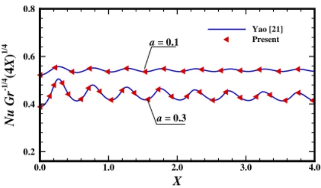
_ρ

= 0.0. This comparison is appeared in Fig. 2 and results matches well with each other and shows good accuracy.

The influence of buoyancy ratio parameter, N r, on skin friction coefficient, τ

w

, heat transfer coefficient, Q

_w

and mass transfer coefficient, M

_w

is illustrated in Fig. 3.

For comparison, the effect of N r on water-based nanofluid without dust particles (i.e., D

ρ

= 0.0) is also presented. It is also important to mention here that the parameter N r is responsible for the coupling between the dimensionless nanoparticle concentration and momentum equation (see Eq. (30)). It can be visualize from Fig. 3(a) that the skin friction coefficient for dusty as well as clear fluid remains almost invariant under the variations of parameter N r. However, variations are recorded for rate of heat transfer as well as for mass transfer coefficient by magnifying the value of buoyancy parameter, N r (see Figs. 3(b) and 3(c)). The effect of, N r, on average, is to reduce the Q

w

and M

w

for clear as well as dusty fluid. But the plots in Fig. 3(b) reveals the fact that the rate of heat transfer is extensively promoted by loading the dust particles into the base fluid (i.e., D

_ρ

= 10.0). Such behavior is expected because the base fluid gains the thermal energy from the dust particles collision which ultimately promote the rate of heat transfer near the vicinity of wavy plate. Higher the values of D

_ρ

, the greater will be the rate of heat transfer. On the other hand, D

_ρ

has a retarding influence on the rate of mass transfer and therefore M

w

is sufficiently reduced when D

ρ

is penetrated into the mechanism. As expected, higher concentration of dust particles causes the mass transfer rate to reduce near the axis of flow.

The results for water-based nanoparticulate suspension are represented in terms of τ

w

, Q

w

and M

w

in Fig. 4. In this figure mass concentration parameter D

ρ

characterizes the influence of particles on their surroundings together with the effect of Eckrect number Ec.

The skin friction coefficient, τ

w

remain uniform for overall range of D

ρ

and Ec (see Fig.

4(a)). However, a large enhancement in the heat transfer rate, Q

w

and a little reduction in the rate of mass transfer coefficient, M

_w

is recorded when mass concentration parameter and Eckrect number increases (see Figs. 4(b) and 4(c)). It is already mentioned that, for the heat transfer rate, the dusty water gains some thermal energy from particles and consequently the temperature gradient for the carrier fluid increases. By loading the dust particles together with higher values of Ec, causes the carrier fluid to be more condense which leads to decrease the rate of mass transfer in stream-wise direction. Moreover, it is intersecting to note that, the non-zero values of Ec only increase (decrease) the rate of heat transfer (rate of mass transfer) for non-zero values of D

_ρ

. It can be concluded from the present study that the Eckrect number Ec has a dominating influence on water particulate suspension as compared to clear fluid.

Fig. 5 is plotted to visualize the effect of amplitude of wavy surface on the distri-

bution of physical quantities, namely, τ

w

, Q

w

and M

w

. The change in surface contour is

followed by raise and fall of the curves. It can be visualize from Fig. 5(a), that the influ-

ence of amplitude a, on average, is to reduce the rate of skin friction. Similar behavior is recorded for the rate of heat transfer (see Fig. 5(b)). As a whole, the rate of heat transfer, Q

w

, reduces when the amplitude of the sinusoidal waveform increases. When the amplitude of wavy surface increases, the shape of the wave gradually changes from sinusoidal waveform to the unusual shape. The reduction in the magnitude of the temperature gradient hap- pened due to the simultaneous influence of centrifugal and buoyancy force. Furthermore, we notice that the change in rate of heat transfer is more pronounced for larger values of the amplitude a and this factor acts as a retarding force for heat transfer coefficient. As expected, the surface having large amplitude causes a reduction in rate of mass transfer (see Fig. 5(c)). It can be seen from Fig. 5(c), that M

w

is maximum for small values of a and depicts a clear decline by increasing the amplitude of wavy surface from 0.3 to 0.8. This may happen due to the fact that the geometry having a transverse nature offers more resistance to water particulate suspension and ultimately the rate of mass transfer decreases.

Fig. 6 anticipates the influence of modified diffusivity ratio parameter, N

_A

, on the distribution of skin friction coefficient, rate of heat transfer and rate of mass transfer coefficient. The graph in Fig. 6(b) shows a clear decline in the values of heat transfer coefficient. It is interesting to note that N

_A

not only reduce the rate of heat transfer but also affect the amplitude of the curves representing Q

_w

. The rate of heat transfer is maximum for N

A

= 0.0 and reduced drastically for non-zero values of modified diffusivity ratio parameter. This is expected because the viscous diffusion rate increases due to an increase in N

_A

which results in significant reduction in Q

_w

. On the other hand, skin friction coefficient and mass transfer coefficient are enhanced for higher values of N

A

as depicted in Figs. 6(a) and 6(c). Specifically, Fig. 6(c) reveals that the effect of N

_A

on mass transfer coefficient is more pronounced for higher values of N

_A

.

The influence of particle-density increment number, N

B

, is observed in Fig. 7. The figure depicts an interesting behavior of N

_B

on (a) τ

_w

, (b) Q

_w

and (c) M

_w

. It is evident from Fig. 7 that except the heat transfer coefficient, all quantities shows a pronounced inclined for increasing values of particle-density increment parameter. By increasing the particle density, the fluid near the surface will undergoes more resistance to flow and produces more frictional forces in boundary layer region, which ultimately enhance the skin friction coefficient(see Fig. 7(a)). As expected to see from Fig. 7(b) that the rate of heat transfer depicted by Q

_w

shows a significant decline by intensifying N

_B

. This may happen because of the presence of the nanoparticles in the base fluid results in a zig-zag motion of the particles, which leads to collisions within the fluid as the particles interact hence increased heat production. Thus, an enhancement in values of particle-density increment number, N

_B

causes more collisions which generate more heat and thus the rate of heat transfer is reduced at the surface of the vertical plate. The non-zero values of N

B

drastically reduce the amplitude of the curve depicting the quantity, Q

w

. Furthermore, it can be seen from Fig. 7(c), that the rate of mass transfer is very low for N

_B

= 0.0, and extensively promoted by increasing the values of N

B

.

Figure 8 is plotted to see the contribution of amplitude of wavy surface, a on velocity

and temperature distribution of dusty water. It can be clearly seen that surface roughness

factor has a notable influence on (U, U

p

) and (Θ, Θ

p

). The velocity profiles, (U, U

p

) suffi-

ciently decreases by magnifying the values of a. This may happens because of the fact that

the frictional forces become more influential due to the geometry having large amplitude,

and the velocity of the dusty water sufficiently decreases between the crusts and troughs

of the wavy pattern (see Fig. 8(a)). while on the other hand, a acts like a supportive

driving force that accelerates the water particulate suspension flow, and, as a result, the

temperature for both phases, (Θ, Θ

p

), within the boundary layer increases significantly (see Fig. 8(b)). The plots for temperature profiles for both, carrier as well as particle phase, quickly approaches to its asymptotic value for a = 0.2, as compared to a = 0.3. It can be concluded that amplitude factor causes a delay for temperature profiles to attain their limiting values into the boundary layer region.

Representative velocity profiles and temperature profiles for carrier as well as dusty phase under the effect of modified diffusivity ratio parameter, N

A

and particle-density increment parameter N

_B

are respectively plotted in Figs. (9) and (10). It can be seen from Fig. 9 that U , U

_p

, Θ and Θ

_p

tends to increase by owing an increase in the values of modified diffusivity ratio parameter. However, it is interesting to see that the velocity as well as temperature profiles for particle phase is always less than the corresponding profiles for fluid phase. This may happens due to the presence of inert-particles in fluid, as they resist the flow and produce friction, which leads to a reduction in the magnitude of U

_p

and Θ

_p

. Thus, it can be concluded that U

_p

and Θ

_p

decays quickly and attain their asymptotic behavior as compared to U and Θ. Similarly, large values of particle-density increment parameter, N

B

accelerates the fluid flow and ultimately promotes the velocity and temperature profiles for both phases (see Fig. 10). It is clear from Fig. 10(a) that the peaks of velocity curves in which non-zero values of N

_B

are considered are relatively high. The non-zero values of particle-density increment parameter, N

B

acts as a delaying factor for velocity and temperature profile of both phases to attain their limiting values in boundary layer regime.

In order to illustrate the influence of mass concentration of dust particles parame- ter, D

_ρ

on streamlines and isotherms for water particulate suspension, Fig. 11 is plotted.

These quantities help in visualizing and accessing the performance of the flow velocity and temperature fields of dusty fluid moving along the wavy surface. For comparison, suspen- sion without particle cloud (pure water) is also presented in Fig. 11. As expected that by loading the dust particles, the velocity of dusty fluid reduces significantly as compared to clear fluid (see Fig. 11(a)). While on the other hand, isotherms in Fig. 11(b) indicates that presence of dust particles have a notable influence on temperature distribution as isotherms get stronger for dusty water. When particles are loaded extensively, (i.e., D

_ρ

= 10.0), the inter-collisions of particles generates thermal energy in the base fluid, which ultimately increases the overall temperature into the boundary layer region.

6 Conclusion

The present analysis aims to compute the numerical results of boundary layer flow of water-

based dusty nanofluid along a vertical wavy surface. Primitive variable formulations are

adopted to transform the dimensionless boundary layer equations into a convenient form,

and then the resulting nonlinear system of boundary layer equations are iteratively solved

step-by-step by using implicit finite difference method along with tri-diagonal solver. Nu-

merical results gives a clear insight towards understanding the response of roughness of the

surface. Effect of various emerging parameters are explored by expressing their relevance

on skin friction coefficient, rate of heat transfer and rate of mass transfer. Velocity and

temperature distributions are also plotted for carrier as well as particle phase. From this

analysis, it is observed that modified diffusivity ratio parameter, N

_A

and particle-density

increment number, N

_B

, has pronounced effect in reduction of heat transfer rate whereas

reverse behavior is recorded in skin friction and rate of mass transfer under the influence

of N

_A

and N

_B

. Moreover, the rate of heat transfer is extensively promoted by loading the mass concentration parameter, D

_ρ

.

References

[1] Choi, S., Enhancing thermal conductivity of fluids with nanoparticles, in: D. A.

Siginer, H. P. Wang (Eds.), Development and Applications of Non-Newtonian Flows, ASME FED-231/MD, 66, 1995, 99-105.

[2] Das, S. K., Choi, S. U., Yu, W., Pradet, T., Nanofluids: Science and Technology, John Wiley & Sons, New Jersey, 2007.

[3] Buongiorno, J., Convective transport in nanofluids, ASME J. Heat Transfer, 128, 2006, 240-250.

[4] Wang, X. Q., Mujumdar, A., A review on nanofluids-Part I: Theoretical and numerical investigations, Braz. J. Chem. Eng., 25, 2008, 613-630.

[5] Kaka¸ c, S., Pramuanjaroenkij, A., Review of convective heat transfer enhancement with nanofluids, Int. J. Heat Mass Tran., 52, 2009, 3187-3196.

[6] Lee, J. H., Lee, S. H., Choi, C. J., Jang, S. P., Choi, S. U. S., A review ofthermal conductivity data, mechanics and models for nanofluids, Int. J. Micro-Nano Scale Transp., 1, 2010, 269-322.

[7] Wong, K. F. V., Leon, O. D., Applications of nanofluids: current and future, Adv.

Mech. Eng., 11, 2010, 519-659.

[8] Begum, N., Siddiqa, S., Hossain, M. A., Nanofluid bioconvection with variable ther- mophysical properties, J. Mol. Liq., 231, 2017, 325-332.

[9] Rudinger, G., Fundamentals of gas-particle flow, Elsevier Scientific Publishing Co., Amsterdam, 1980.

[10] Farbar, L., Morley, M. J., Heat transfer to flowing gas-solid mixtures in a circular tube, Ind. Eng. Chem., 49, 1957, 1143-1150.

[11] Saffman, P. G., On the stability of laminar flow of a dusty gas, J. Fluid Mech., 13, 1962, 120-128.

[12] Marble, F. E., Dynamics of a gas containing small solid particles, combustion and propulsion, 5th AGARD colloquium, Pergamon press, 1963.

[13] Singleton, R. E., Fluid mechanics of gas-solid particle flow in boundary layers, Ph.D.

Thesis, California Institute of Technology, 1964.

[14] Gireesha, B. J., Bagewadi, C. S., Prasannakumar, B. C., Study of unsteady dusty fluid Flow through rectangular channel in Frenet Frame Field system, Int. J. Pure Appl. Math., 34, 2007, 525-534.

[15] Gireesha, B. J., Bagewadi, C. S., Prasannakumar, B. C., Pulsatile flow of an unsteady

dusty fluid through rectangular channel, Commun. Nonlinear Sci. Numer. Simulat.,

14, 2009, 2103-2110.

[16] Manjunatha, P. T., Gireesha, B. J., Prasannakumar, B. C., Thermal analysis of con- ducting dusty fluid flow in a porous medium over a stretching cylinder in the presence of non-uniform source/sink, International journal of mechanical and materials engi- neering, 2014, 1-13.

[17] Prasannakumar, B. C., Gireesha, B. J., Manjunatha, P. T., Melting phenomenon in MHD stagnation point flow of dusty fluid over a stretching sheet in the presence of thermal radiation and non-uniform heat source/sink, Int. J. Comput. Methods Eng.

Sci Mech., 16, 2015, 265-274.

[18] Bagewadi, C. S., Venkatesh, P., Shashikumar, N. S., Prasannakumar, B. C., Boundary layer flow of dusty fluid over a radiating stretching surface embedded in a thermally stratified porous medium in the presence of uniform heat source, Nonlinear Engineer- ing, 6, 2017, 31-41.

[19] Siddiqa, S., Begum, N., Hossain, M. A., Massarotti, N., Influence of thermal radiation on two-phase flow along a vertical wavy frustum of a cone, Int. Commun. Heat Mass, 76, 2016 63-68.

[20] Siddiqa, S., Begum, N., Hossain, M. A., Gorla, R. S. R., Thermal Maragoni convection of two-phase dusty fluid flow along a vertical wavy surface, J. Appl. Fluid Mech., 10, 2017, 509-517.

[21] Yao, L. S., Natural convection along a vertical wavy surface, J. Heat Transfer, 105, 1983, 465-468.

[22] Rees, D. A. S., Pop, I., Free convection induced by a vertical wavy surface with uniform heat flux in a porous medium, J. Heat Transfer, 117, 1995, 545-550.

[23] Pop, I., Natural convection of a darcian fluid about a wavy cone, Int. Commun. Heat Mass, 21, 1994, 891-899.

[24] Pop, I., Na, T. Y., Natural convection from a wavy cone, Appl. Sci. Res., 54, 1995, 125-136.

[25] Pop, I., Na, T. Y., Natural convection over a vertical wavy frustum of a cone, J.

Nonlinear Mechanics, 34, 1999, 925-934.

[26] Siddiqa, S., Begum, N., Hossain, M. A., Gorla, R. S. R., Natural convection flow of a two-phase dusty non-Newtonian fluid along a vertical surface, Int. J. Heat Mass Tran., 113, 2017, 482-489.

[27] Siddiqa, S., Begum, N., Hossain, M. A., Compressible Dusty Fluid along a Vertical Wavy Surface, Appl. Math. Comput., 293, 2017, 600-610.

[28] Apazidis, N., Temperature distribution and heat transfer in a particle-fluid flow past

a heated horizontal plate, Int. J. Multiphas. Flow, 16, 1990, 495-513.

X Nu Gr-1/4 (4X)1/4

0.0 1.0 2.0 3.0 4.0

0.2 0.4 0.6 0.8

Yao [21]

Present a = 0.1

a = 0.3

Fig. 2 Local Nusselt number coefficient for a = 0.1, 0.3, while D

_ρ

= 0.0, Pr = 1.0, α

d

= 0.0, N r = 0.0, N

A

= N

B

= 0.0 and γ = 1.0.

X τw

0.0 0.5 1.0 1.5 2.0 2.5

0.2 0.4 0.6 0.8 1.0 1.2

Nr = 0.0, D_ρ = 0.0 Nr = 0.0, Dρ = 10.0 Nr = 0.1, Dρ = 0.0 Nr = 0.1, D_ρ = 10.0

(a X

Qw

0.0 0.5 1.0 1.5 2.0

0.10 0.11 0.12 0.13 0.14

Nr = 0.0, D_ρ = 0.0 Nr = 0.0, Dρ = 10.0 Nr = 0.1, Dρ = 0.0 Nr = 0.1, Dρ = 10.0

(

X Mw

0.0 0.5 1.0 1.5 2.0

2.0 2.2 2.4 2.6 2.8

Nr = 0.0, D_ρ = 0.0 Nr = 0.0, D_ρ = 10.0 Nr = 0.1, D_ρ = 0.0 Nr = 0.1,

Fig. 3(a) τ

_w

, (b) Q

_w

and (c) M

_w

for N r = 0.0, 0.1, D

_ρ

= 0.0, 10.0 while Pr = 7.0,

γ = 0.1, α

_d

= 0.01, Ec = 1.0, N

_A

= 5.0, N

_B

= 10.0, Ln = 100.0 and a = 0.3.

X τw

0.0 0.5 1.0 1.5 2.0 2.5

0.2 0.4 0.6 0.8 1.0 1.2

Ec = 0.0, D_ρ = 0.0 Ec = 0.0, D_ρ = 10.0 Ec = 1.0, D_ρ = 0.0 Ec = 1.0, D_ρ = 10.0

(a X

Qw

0.0 0.5 1.0 1.5 2.0 2.5

0.10 0.11 0.12 0.13 0.14 0.15

Ec = 0.0, D_ρ = 0.0 Ec = 0.0, D_ρ = 10.0 Ec = 1.0, D_ρ = 0.0 Ec = 1.0, D_ρ = 10.0

(b)

X Mw

0.0 0.5 1.0 1.5 2.0

2.0 2.2 2.4 2.6

Ec = 0.0, D_ρ = 0.0 Ec = 0.0, D_ρ = 10.0 Ec = 1.0, D_ρ = 0.0 Ec = 1.0, D_ρ

Fig. 4(a) τ

w

, (b) Q

w

and (c) M

w

for Ec = 0.0, 1.0, D

ρ

= 0.0, 10.0 while Pr = 7.0, γ = 0.1, α

_d

= 0.01, N r = 0.1, N

A

= 5.0, N

B

= 10.0, Ln = 100.0 and a = 0.3.

X τw

0.0 0.5 1.0 1.5 2.0 2.5

0.0 0.2 0.4 0.6 0.8 1.0

a = 0.3 a = 0.5 a = 0.8

(a X

Qw

0.0 0.5 1.0 1.5 2.0 2.5

0.06 0.08 0.10 0.12 0.14 0.16

a = 0.3 a = 0.5 a = 0.8

(b

X Mw

0.0 0.5 1.0 1.5 2.0 2.5

1.0 1.5 2.0 2.5

a = 0.3 a = 0.5 a = 0.8

(c)

Fig. 5(a) τ

w

, (b) Q

w

and (c) M

w

for a = 0.3, 0.5, 0.8 while D

ρ

= 10.0 Pr = 7.0,

γ = 0.1, α

_d

= 0.01, Ec = 1.0, N r = 0.1, N

A

= 5.0, N

B

= 10.0 and Ln = 100.0.

X τw

0.0 0.5 1.0 1.5 2.0 2.5

0.2 0.4 0.6 0.8 1.0 1.2

N_A = 0.0 N_A = 5.0 N_A = 10.0

(a X

Qw

0.0 0.5 1.0 1.5 2.0 2.5 3.0

0.0 0.1 0.2 0.3 0.4

NA = 0.0 N

X Mw

0.0 0.5 1.0 1.5 2.0 2.5

1.5 2.0 2.5

3.0 NA = 0.0

NA = 5.0 NA = 10.0

(c)

Fig. 6(a) τ

w

, (b) Q

w

and (c) M

w

for N

A

= 0.0, 5.0, 10.0 while D

ρ

= 10.0 Pr = 7.0, γ = 0.1, α

_d

= 0.01, Ec = 1.0, N r = 0.1, N

B

= 10.0, Ln = 100.0 and a = 0.3.

X τw

0.0 0.5 1.0 1.5 2.0 2.5

0.2 0.4 0.6 0.8 1.0

N_B = 0.0 N_B = 5.0

X Qw

0.0 0.5 1.0 1.5 2.0 2.5 3.0

0.0 0.2 0.4 0.6

NB = 0.0 N

X Mw

0.0 0.5 1.0 1.5 2.0 2.5 3.0

1.0 1.5 2.0 2.5

NB = 0.0 NB = 5.0 NB = 10.0

(c)

Fig. 7(a) τ

w

, (b) Q

w

and (c) M

w

for N

B

= 0.0, 5.0, 10.0 while D

ρ

= 10.0 Pr = 7.0,

γ = 0.1, α

_d

= 0.01, Ec = 1.0, N r = 0.1, N

A

= 5.0, Ln = 100.0 and a = 0.3.

Y U, Up

0.0 2.0 4.0 6.0 8.0 10.0 12.0 14.0

0.00 0.06 0.12 0.18

a = 0.2 a = 0.3 U

Up

(a) Y

Θ, Θp

0.0 2.0 4.0 6.0 8.0 10.0 12.0 14.0

0.0 0.2 0.4 0.6 0.8 1.0

a

Fig. 8(a) Velocity and (b) temperature profiles for a = 0.2, 0.3, while D

_ρ

= 10.0, Pr = 7.0, γ = 0.1, α

d

= 0.1, Ec = 1.0, N

A

= 5.0, N

B

= 5.0, Ln = 100.0, N r = 0.1 and

X = 10.0.

Y U, Up

0.0 2.0 4.

Y Θ, Θp

0.0 2.0 4.0 6.0 8.0 10.0

0.0 0.2 0.4 0.6 0.8 1.0

NA = 0.0 NA = 5.0

(b)

Θp

Fig. 9(a) Velocity and (b) temperature profiles for N

_A

= 0.0, 5.0, while D

ρ

= 10.0, Pr = 7.0, γ = 0.1, α

d

= 0.1, Ec = 1.0, N

B

= 5.0, a = 0.2, Ln = 100.0,

N r = 0.1 and X = 10.0.

Y U, Up

0.0 2.0 4.0 6.0 8.0 10.0

0.00 0.05 0.10 0.15

NB = 0.0 NB = 5.0 U

Up

(a Y

Θ, Θp

0.0 2.0 4.0 6.0 8.0 10.0

0.0 0.2 0.4 0.6 0.8 1.0

NB = 0.0 NB = 5.0

(b)

Θp

Fig. 10(a) Velocity and (b) temperature profiles for N

_B

= 0.0, 5.0, while D

ρ

= 10.0, Pr = 7.0, γ = 0.1, α

d

= 0.1, Ec = 1.0, N

A

= 2.0, a = 0.2, Ln = 100.0,

N r = 0.1 and X = 10.0.

X

Y

1.0 2.0 3.0 4.0 5.0

0.0 5.0 10.0 15.0 20.0 25.0 30.0

(a)

Water with particles (D_ρ = 10.0) Pure water (D_ρ = 0.0)

X

Y

0.5 1.0 1.5 2.0 2.5 3.0 3.5

0.0 2.0 4.0 6.0 8.0 10.0

(b)

Pure water (D_ρ = 0.0) Water with particles (D_ρ = 10.0

Fig. 11(a) Streamlines and (b) Isotherms for D

ρ

= 0.0, 10.0, Pr = 7.0, γ = 0.1,

α

_d

= 0.01, Ec = 1.0, N

_A

= 5.0, N

_B

= 10.0, Ln = 100.0, a = 0.3 and N r = 0.1.