Two-Phase Dusty Fluid Flow Along a Cone with Variable Properties

No. 566 May 2017

Two-Phase Dusty Fluid Flow Along a Cone with Variable Properties

S. Siddiqa, N. Begum, Md. A. Hossain,

N. Mustafa, R. S. R. Gorla

Two-Phase Dusty Fluid Flow Along a Cone with Variable Properties

Sadia Siddiqa ^∗ , Naheed Begum ^§ , Md. Anwar Hossain ^‡ , Naeem Mustafa ^∗∗ , Rama Subba Reddy Gorla ^{† ,1}

∗ Department of Mathematics, COMSATS Institute of Information Technology, Kamra Road, Attock, Pakistan

§ Institute of Applied Mathematics (LSIII), TU Dortmund, Vogelpothsweg 87, D-44221 Dortmund, Germany

‡ UGC Professor, University of Dhaka, Dhaka, Bangladesh

∗∗ Principal Scientist, Theoretical Physics Division, PINSTECH, P.O. NILORE, Islamabad, Pakistan,

† Department of Mechanical Engineering, University of Akron, Akron, Ohio 44325 USA Abstract: In this paper numerical solutions of a two-phase natural convection dusty fluid flow are presented. The two-phase particulate suspension is investigated along a vertical cone by keeping variable viscosity and thermal conductivity of the carrier phase. Compre- hensive flow formations of the gas and particle phases are given with the aim to predict the behavior of heat transport across the heated cone. The influence of i) air with particles, water with particles and oil with particles are shown on shear stress coefficient and heat transfer coefficient. It is recorded that sufficient increment in heat transport rate can be achieved by loading the dust particles in the air. Further, distribution of velocity and tem- perature of both the carrier phase and the particle phase are shown graphically for the pure fluid (air, water) as well as for the fluid with particles (air-metal and water-metal particle mixture).

Keywords: Natural Convection, Dusty Fluid, Two-Phase, Variable Viscosity, Variable Thermal Conductivity, Vertical Cone

1 Introduction

The analysis of the flow of fluids with suspended particles or gas-particle mixture have re- ceived notable attention due to its practical applications in various problem of atmospheric, engineering and physiological fields. Solid rocket exhaust nozzles, combustion chambers, blast waves moving over the Earth’s surface, conveying of powdered materials, fluidized beds, environmental pollutants, petroleum industry, purification of crude oil and other tech- nological fields are some of the practical applications of dusty fluids (see [1]). Farbar and Morley [2] were the first to analyze the gas-particulate suspension on experimental grounds.

Saffman [3] reported the stability of laminar flow and formulated the governing equations for the flow of dusty fluid. After that, Marble [4] studied the problem of dynamics of a gas containing small solid particles and developed the equations for gas-particle flow systems.

Singleton [5] was the first to study the boundary layer analysis for dusty fluid and later on, the dynamics of two-phase flow was investigated by [6]. A more recent analysis for natural convection flow of a dusty fluid along a vertical surface has been considered by Siddiqa et al.

1

Corresponding author.

Email: rama.gorla@yahoo.com

[7]). They obtained the numerical solutions for the wide range of Prandtl number Pr (Here Pr = (c _p µ _∞ )/κ _∞ ; where c _p the specific heat at constant pressure, µ _∞ and κ _∞ the dynamic viscosity and thermal conductivity of fluid in free stream region, respectively) starting from 0.7 to 1000.0.

It is worthy to mention that all the above analysis were made on the assumption that both the viscosity and thermal conductivity of the fluid are uniform. But, the flu- ids having significant role in the theory of lubrication, for instance, do not correspond to uniform nature of viscosity and thermal conductivity since the heat generated by the internal friction and the corresponding rise in temperature deliberately alter these proper- ties. In addition, many problems in engineering occur at very high temperatures and hence the knowledge of viscosity effects on the convective heat transfer becomes very important for the design of the pertinent equipment. For instance, the viscosity of water increases by about 240% when the temperature decreases from 500 ^◦ C(µ = 0.000548kgm ^{− 1} s ^{− 1} ) to 100 ^◦ C(µ = 0.00131kgm ^{− 1} s ^{− 1} ). Several studies, have introduced temperature dependent properties and reported significant influence of these properties over the flow characteris- tics. For instance, Kays and Grawford [10] presented a variety of mathematical formulas between the temperature and physical properties of fluids by keeping various practical sit- uations in mind. It has been found that for a fluid, both the thermal conductivity and viscosity varies linearly with the corresponding changes in temperature. Considering this fact, Charraudeau [11] suggested the linear form of fluid viscosity and thermal conductivity through two semi-empirical formulas:

µ = µ _∞ [

1 + ϵ(T − T _∞ ) T _w − T _∞

]

κ = κ _∞ [

1 + γ(T − T _∞ ) T _w − T _∞

]

(1) where T the temperature of the fluid, T w the temperature of the surface of cone and T _∞ the ambient fluid temperature. Further, µ _∞ and κ _∞ are the viscosity and thermal conductivity of the ambient fluid and ϵ and γ are respectively the viscosity variation parameter and thermal conductivity variation parameter. Some authors, for example, Hossian et al. [12], Hossain and Munir [13] and Siddiqa et al. [14] reported the effects of variable properties by using (1), under different physical circumstances. In present analysis as well, both the viscosity and thermal conductivity variations of the carrier fluid are exploited through the proposed form of Charraudea [11].

In this paper consideration has been given to the effects of temperature dependent viscosity and thermal conductivity of dusty fluid on laminar natural convection flow along a vertical heated cone. Such problems found their applications in many industrial problems where temperature dependent properties of dusty fluid is a subject of practical interest.

Coordinate transformation (primitive variable formulation) is employed to transform the

two-phase boundary layer model into a convenient form. Since the equations (22-28) are

coupled and nonlinear therefore solutions are obtained numerically by applying two point

implicit finite difference method. Numerical results of the two-phase problem are displayed

in the form of wall shear stress, heat transfer rate, streamlines, isotherms by varying several

controlling parameters.

2 Formulation of the Problem

We have considered dusty fluid which is originally at rest along a vertical heated solid cone.

Initially, the system is having a uniform temperature T _∞ . Suddenly, the surface of the cone y = 0 is heated to a temperature T + ∆T and natural convection starts due to this. The x-axis is taken along the surface of the cone, whereas y-axis is in the direction normal to the surface as shown in Fig. 1. In our detailed numerical work, the fluid viscosity and thermal conductivity are taken as a linear function of temperature (given in Eq. 1). Under the assumptions given in Siddiqa et al. [7], the governing system of equations pertinent to the problem are given by (see Ref. [3], [7]-[9]):

For the fluid phase:

∂(ˆ r u) ˆ

∂ x ˆ + ∂(ˆ r v) ˆ

∂ y ˆ = 0 (2)

ρ (

ˆ u ∂ u ˆ

∂ x ˆ + ˆ v ∂ u ˆ

∂ y ˆ )

= − ∂ p ˆ

∂ x ˆ + ∇ .(µ ∇ u) + ˆ ρgβ (T − T _∞ ) cos ϕ + ρ _p τ m

(ˆ u _p − u) ˆ (3) ρ

( ˆ u ∂ˆ v

∂ x ˆ + ˆ v ∂ˆ v

∂ y ˆ )

= − ∂ p ˆ

∂ˆ y + ∇ .(µ ∇ ˆ v) − ρgβ (T − T _∞ ) sin ϕ + ρ p

τ _m (ˆ v p − v) ˆ (4) ρc _p

( ˆ u ∂T

∂ˆ x + ˆ v ∂T

∂ˆ y )

= ∇ .(κ ∇ T ) + ρ _p c _s τ T

(T _p − T ) (5)

For the particle phase:

∂(ˆ r u ˆ _p )

∂ x ˆ + ∂(ˆ r v ˆ _p )

∂ y ˆ = 0 (6)

ρ p

( ˆ u p

∂ˆ u p

∂ x ˆ + ˆ v p

∂ u ˆ p

∂ y ˆ )

= − ∂ p ˆ p

∂ˆ x − ρ p

τ _m (ˆ u p − u) ˆ (7) ρ _p

( ˆ u _p ∂ v ˆ _p

∂ x ˆ + ˆ v _p ∂ˆ v _p

∂ y ˆ )

= − ∂ p ˆ _p

∂ y ˆ − ρ _p τ m

(ˆ v _p − v) ˆ (8)

ρ p c s

( ˆ u p

∂T p

∂ x ˆ + ˆ v p

∂T p

∂ y ˆ )

= − ρ p c s

τ _T (T p − T ) (9)

where (ˆ u, ˆ v), T , ˆ p, ρ, c p , β κ, µ are respectively the velocity vector in the (ˆ x, y) direction, ˆ temperature, pressure, density, specific heat at constant pressure, volumetric expansion coefficient, thermal conductivity and coefficient of dynamic viscosity of the fluid/carrier phase. Similarly, (ˆ u p , v ˆ p ), T p , ˆ p p , ρ p and c s corresponds to the velocity vector, temperature, pressure, density and specific heat for the particle phase. ⃗ g = (g cos ϕ, g sin ϕ) is the gravi- tational acceleration along the (ˆ x, y) directions respectively, ˆ ϕ the half angle and ˆ r = ˆ x sin ϕ the local radius of the cone. Likewise, τ m (τ T ) is the momentum relaxation time (thermal relaxation time) during which the velocity (temperature) of the particle phase relative to the fluid is reduced to 1/e times its initial value. The fundamental equations stated above are to be solved under appropriate boundary conditions to determine the flow fields of the fluid and the dust particles. Therefore, boundary conditions for the gas phase are:

ˆ

u(ˆ x, 0) = ˆ v(ˆ x, 0) = T (ˆ x, 0) − T w = 0

u(ˆ x, ∞ ) = T (ˆ x, ∞ ) − T _∞ = 0 (10)

Boundary conditions for the particle phase are:

ˆ

u p (ˆ x, 0) = ˆ v p (ˆ x, 0) = T p (ˆ x, 0) − T w = 0 ˆ

u p (ˆ x, ∞ ) = T p (ˆ x, ∞ ) − T _∞ = 0 (11) T w is the constant temperature of the heated cone which is higher than the ambient fluid temperature T _∞ . The above system of governing equations is transformed into a dimen- sionless system of equations by using the following transformation:

(u, u p ) = L

ν _∞ Gr ^{− 1/2} (ˆ u, u ˆ p ), (v, v p ) = L

ν _∞ Gr ^{− 1/4} (ˆ v, v ˆ p ), (Θ, Θ p ) = (T, T p ) − T _∞ T _w − T _∞ , x = x ˆ

L , y = y ˆ

L Gr ^1/4 , r = r ˆ

L , (p, p _p ) = L ²

ρν _∞ ² Gr (ˆ p, p ˆ _p ), Gr = gβ(T _w − T _∞ ) cos ϕL ³

ν _∞ ² , Pr = µ _∞ c _p

κ _∞ , ν _∞ = µ _∞ ρ

(12)

System of Eqs. (2)-(11) becomes:

∂(ru)

∂x + ∂(rv)

∂y = 0 (13)

u ∂u

∂x + v ∂u

∂y = − ∂p

∂x + ϵ ∂u

∂y

∂θ

∂y + (1 + εθ) ∂ ² u

∂y ² + D _ρ α _d (u _p − u) + θ (14) u ∂θ

∂x + v ∂θ

∂y = 1 Pr

(

(1 + γθ) ∂ ² θ

∂y ² + γ ( ∂θ

∂y ) 2

− 2

3 D ρ α _d (θ − θ p ) )

(15)

∂(ru p )

∂x + ∂(rv p )

∂y = 0 (16)

u _p ∂u _p

∂x + v _p ∂u _p

∂y = − ∂p _p

∂x − α _d (u _p − u) (17) u _p ∂θ _p

∂x + v _p ∂θ _p

∂y = − 2

3ωPr α _d (θ _p − θ) (18)

The boundary conditions for the gas phase becomes:

u(x, 0) = v(x, 0) = θ(x, 0) − 1 = 0

u(x, ∞ ) = θ(x, ∞ ) = 0 (19)

Similarly, for the particle phase boundary conditions can be written as:

u _p (x, 0) = v _p (x, 0) = θ _p (x, 0) − 1 = 0

u _p (x, ∞ ) = θ _p (x, ∞ ) = 0 (20)

The interaction terms between the two phases (carrier phase and particle phase) are ex- pressed as follows:

ω(= c s /c p ) is the specific heat ratio of the mixture. For different gas-particle combinations, ω may vary between 0.1 and 10.0, and in such cases, either the temperature or the velocity tends to reach equilibrium faster (see [1]).

D _ρ (= ρ _p /ρ) is mass concentration of particle phase or the ratio of densities of the fluid and

the dust particles.

τ T = 1.5ωτ m P r is the relation between thermal relaxation time (τ T ) and velocity relaxation time (τ _m ); indicating that τ _T is obeying the Stokes law. It should be noted that, for most gases, the Prandtl number, Pr is near 2/3 and the specific heat mixture parameter (ω) is typically near one, which means that for this particular situation temperature and velocity relaxation become equivalent.

Finally, α _d = L ² /ντ _m Gr ^1/2 is the parameter depending on the relaxation time of the par- ticles and the buoyancy force. It can be observed that for α _d = 0 the flow governs by the natural convection in the absence of the dusty particles.

Before applying the numerical scheme, following set of continuous transformations are introduced:

(u, u p ) = x

(U, U p ), (v, v p ) = x ⁻

(V, V p ), (θ, θ p ) = x ⁿ (Θ, Θ p ) y = x

Y, X = α _d x

(21) Eqs. (13)-(20) becomes:

3 + n

2 U + 1 − n 2 X ∂U

∂X − 1 − n 4 Y ∂U

∂Y + ∂V

∂Y = 0 (22)

1 + n

2 U ² + 1 − n

2 XU ∂U

∂X + (

V − 1 − n 4 Y U

) ∂U

∂Y = (1+ϵΘ) ∂ ² U

∂Y ² +ϵ ∂U

∂Y

∂Θ

∂Y +Θ − D ρ X(U − U p ) (23) nUΘ + 1 − n

2 XU ∂Θ

∂X + (

V − 1 − n 4 Y U

) ∂Θ

∂Y = 1

Pr [

(1 + γΘ) ∂ ² Θ

∂Y ² + γ ( ∂Θ

∂Y ) ₂

− 2

3 D ρ X (Θ − Θ p )

] (24)

3 + n

2 U p + 1 − n 2 X ∂U p

∂X − 1 − n 4 Y ∂U p

∂Y + ∂V p

∂Y = 0 (25)

1 + n

2 U _p ² + 1 − n

2 XU _p ∂U p

∂X + (

V _p − 1 − n 4 Y U _p

) ∂U _P

∂Y = − X(U _p − U ) (26) nU p Θ p + 1 − n

2 XU p

∂Θ _p

∂X + (

V p − 1 − n 4 Y U p

) ∂Θ _p

∂Y = − 2X

3ωPr (Θ p − Θ) (27) The boundary conditions to be satisfied are:

U (X, 0) = V (X, 0) = Θ(X, 0) − 1 = U p (X, 0) = V p (X, 0) = Θ p (X, 0) − 1 = 0

U (X, ∞ ) = U _p (X, ∞ ) = Θ(X, 0) = Θ _p (X, ∞ ) = 0 (28) The coupled system of non linear partial differential Eqs. (22)-(27) is solved numerically by using an implicit, iterative tri-diagonal finite difference scheme. The brief description of the numerical scheme is given in Appendix A. In the next section, numerical solutions obtained for the present model are graphed and discussed as well.

3 Numerical Results and Discussion

Present analysis is performed for natural convection flow of dusty fluid along a semi-infinite

vertical flat cone. Equations (22)-(27) under the conditions (28) have been solved nu-

merically using the finite difference method together with the Thomas algorithm. All the

numerical computations are carried out in Fortran 77 code. The quantities of physical in- terest are surface shear stress and the rate of heat transfer which may be attained with the help of following relations:

Q _w = N uGr ^{− 1/4} ( X

α d

)

2−2n

= − (1 + γ ) ( ∂Θ

∂Y )

Y =0

τ _w = C _f Gr ^{− 3/4} ( X

α d

)

2−2n

= (1 + ϵ) ( ∂U

∂Y )

Y =0

(29)

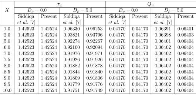
The present numerical results are also validated through comparison with two studies avail- able in literature. It is observed that the our model present the solutions of Pop and Na [16] if P r = 0.72, ϕ = 10 ^◦ , D ρ = 0.0, ϵ = 0.0, γ = 0.0, n = 0.0. The results for the above set of data are presented graphically in Fig. 2. Similarly, solutions of Siddiqa et al. [7] are obtained in Table 1 for dusty fluid by fixing the parameters as D _ρ = 0.0, 5.0, n = 0.0, 1.0, P r = 0.005 and γ = 1.0. The angle ϕ is zero in order to get the solutions of [7]. It is clear from the Fig. 2 and Table 1 that both solutions agree very well with the present study.

Table 1: Numerical values of τ _w and Q _w for D _ρ = 0.0, 5.0, n = 0.0, P r = 0.005, γ = 1.0

X

τ w Q w

D _ρ = 0.0 D _ρ = 5.0 D _ρ = 0.0 D _ρ = 5.0

Siddiqa Present Siddiqa Present Siddiqa Present Siddiqa Present

et al. [7] et al. [7] et al. [7] et al. [7]

1.0 1.42523 1.42524 0.96330 0.96253 0.04170 0.04170 0.06391 0.06401 2.0 1.42523 1.42524 0.93821 0.93796 0.04170 0.04170 0.06398 0.06403 5.0 1.42523 1.42524 0.92274 0.92267 0.04170 0.04170 0.06401 0.06404 6.0 1.42523 1.42524 0.92100 0.92094 0.04170 0.04170 0.06402 0.06404 7.0 1.42523 1.42524 0.91976 0.91971 0.04170 0.04170 0.06402 0.06404 7.5 1.42523 1.42524 0.91926 0.91926 0.04170 0.04170 0.06402 0.06404 8.0 1.42523 1.42524 0.91882 0.91878 0.04170 0.04170 0.06402 0.06404 8.5 1.42523 1.42524 0.91844 0.91840 0.04170 0.04170 0.06402 0.06404 9.0 1.42523 1.42524 0.91809 0.91806 0.04170 0.04170 0.06402 0.06404 9.5 1.42523 1.42524 0.91779 0.91776 0.04170 0.04170 0.06402 0.06404 10.0 1.42523 1.42524 0.91751 0.91749 0.04170 0.04170 0.06402 0.06404

Numerical results are presented for a wide range of Prandtl number Pr (from 0.7 to 1000.0). Variation of wall shear stress, Nusselt number coefficient, velocity profile and temperature profile are obtained for various values of representative parameters. Follow- ing are some practical examples that helps in considering the orders of magnitude of the dimensionless numbers which form the coefficients of the momentum and energy equations (see Apazidis [15]).

• metal particles in gas: D _ρ = 10 ⁴ , Pr = 0.7, ω = 0.45.

• metal particles in water: D _ρ = 10, Pr = 7.0, ω = 0.1.

• metal particles in oil: D ρ = 10, Pr = 1000.0, ω = 0.3.

The numerical values of τ w and Q w for ϵ = 0.0, 5.0, n = 0.0, 1.0, γ = 5.0, Pr = 5.0, ω = 0.5 and D _ρ = 20.0 are entered in Table 2. Numerical values of τ _w (Q _w ) at Y = 0 indicate that slip velocity (heat flux rate) increases (decreases) due to the increment in ϵ from 0.0 to 5.0.

The quantitative data clearly shows the influence of power index n on τ w and Q w . In case of τ _w , the numeric values reduces in magnitude when n increases from 0.0 to 1.0, while on the other hand opposite behavior is recorded for Q _w . The numerical solutions are discussed Table 2: Numerical values of τ w and Q w for ϵ = 0.0, 5.0, n = 0.0, 1.0, γ = 5.0, Pr = 5.0, ω = 0.5, D _ρ = 1000.0

X

τ w Q w τ w Q w

n = 0.0 n = 1.0

ϵ = 0.0 ϵ = 5.0 ϵ = 0.0 ϵ = 5.0 ϵ = 0.0 ϵ = 5.0 ϵ = 0.0 ϵ = 5.0 1.0095 0.15572 0.26991 10.19567 7.67404 0.13906 0.24027 12.72770 9.51374 2.0090 0.15451 0.26845 10.20298 7.67485 0.13779 0.23858 12.83279 9.54633 3.0085 0.15412 0.26797 10.20609 7.67436 0.13734 0.23805 12.86656 9.56141 4.0080 0.15392 0.26777 10.20617 7.67693 0.13715 0.23774 12.88276 9.56335 5.0075 0.15383 0.26761 10.21004 7.67654 0.13700 0.23752 12.88870 9.56334

for the mixture of gas, water and oil with metal particles. Graphical presentation of τ _w and Q _w is given in Fig. 3 for air particle and water particle mixtures. It is worth mentioning that the curves in which air is acting as a carrier fluid exhibits considerable change due to the presence of metal particles as compared to water particulate suspension. In Fig. 3(a), it can be seen that skin friction decreases by increasing the value of mass concentration parameter D _ρ . Such behavior is expected because the carrier fluid loses kinetic and thermal energy by interacting with the dust particles and this leads to reduction of velocity of carrier fluid as compared to pure fluid case. Ultimately the velocity gradient for the carrier fluid decreases at the surface of the cone. It is evident from the Fig. 3(b) that Nusselt number coefficient drastically increases by increasing the mass concentration parameter D _ρ for air particulate suspension. Here the dusty air gains some thermal energy from particles and the temperature of the carrier fluid increases. Consequently, the temperature gradient for the carrier fluid increases. On contrary, the graphical representation for water particulate suspension depicts that the Q w almost remains invariant when D ρ penetrated into the mechanism.

Interestingly, the effect of D _ρ on τ _w and Q _w for oil particulate suspension is reverse when compared to air and water particulate suspensions. Fig. 4 is depicting the contam- ination of oil by metal particles. For comparison, suspension without particle cloud (pure oil) is also presented. The magnitude of τ w (Q w ) drastically increases (decreases) when oil contains metal particles. Furthermore, the behavior of oil mixture on Fig. 4(b) is notice- able since heat transfer rate, Q _w , becomes negative. It happens because hot stream due to buoyancy rises and most probably the temperature of the carrier fluid becomes higher than the temperature at the surface of the cone and it results in negative heat transfer rate.

Streamlines and isotherms are also drawn in Fig. 5 and 6 respectively for air partic-

ulate suspension and water particulate suspension. These quantities help in visualizing and

accessing the performance of the flow velocity and temperature fields of dusty fluid moving

along a vertical cone. For comparison, suspension without particle cloud (pure air/water) is also presented. As expected that by loading the metal particles, the velocity of dusty fluid reduces significantly as compared to clear fluid (pure air/water) as shown in Fig. 5(a) and 6(a). More interestingly, the influence of D ρ on temperature distribution for both phases for air particulate suspension in Fig. 5(b) is notable. When particles are loaded extensively, the relative velocity between the two phases reduces and relaxation time for energy transfer also decreases and ultimately temperature lags between the mixture components become smaller. The thermal boundary layer becomes thinner due to the large temperature lags between the phases. On contrary, isotherms in Fig. 6(b) is revealing the fact that for the two-phase and single phase, curves are very close to each other. It indicates that presence of metal particles do not have much influence on temperature distribution when the carrier fluid is water.

4 Conclusion

This paper aims to compute numerical results of two-phase boundary layer flow of dusty fluid along a vertical heated cone. Primitive variable formulations are adopted to transform the dimensionless boundary layer equations into convenient form and then the resulting nonlinear system of boundary layer equations are iteratively solved step by step by using implicit finite difference method along with tri-diagonal solver. The problem is investigated to predict the characteristics of natural convection dusty fluid flow having variable fluid properties. Results are interpreted by considering base fluid/continuous fluid as water, air and oil, while particle cloud contains metal as a solid phase. The key observation from the present analysis is that inclusion of dust particles in water and air extensively promote the heat transfer rate, particulary, Q _w boosts up when the carrier fluid is air. It is also found that the effect of particle loading is to reduced the wall shear parameter for air and water, but on the other hand, drag forces increases when the participating fluid is oil. The solutions present some features which were not encountered when the fluid properties are taken as uniform. The results of the study may be of some interest to the researchers of the field of chemical engineers and it can be further extended for the generalized three dimensional case.

Appendix A: The discretization procedure is carried out by incorporating two-point back- ward difference formulae for all the first order derivatives with respect to X as:

( ∂Ω

∂X )

i,j

= Ω i,j − Ω i − 1,j

∆X

Similarly, derivatives with respect to Y are replaced by central difference quotients of the form:

( ∂Ω

∂Y )

i,j

= Ω i,j+1 − Ω i,j − 1

∆Y where

Ω _i,j = Ω(X _i , Y _j ) Y _j = (j − 1)∆Y for j = 1, 2, 3...N

Y _∞ = Y _N X _i = (i − 1)∆X for i = 1, 2, 3...M

Here Ω i,j denotes the dependent variable U , U p , Θ, Θ p , and i, j are the node locations along the X and Y directions, respectively. The system of equations is cast into a tridiagonal matrix equation of the form:

A _i,j Ω _{i,j − 1} + B _i,j Ω _i,j + C _i,j Ω _i,j+1 = D _i,j where

Ω _i,j =



 

 U Θ U _p Θ p



 

 A _i,j =



 



A 11 0 0 0

0 A ₂₂ 0 0

0 0 A ₃₃ 0

0 0 0 A 44



 

 B _i,j =



 



B 11 B 12 B 13 B 14

0 B ₂₂ B ₂₃ B ₂₄ 0 0 B ₃₃ B ₃₄

0 0 0 B 44



 



C i,j =



 



C ₁₁ 0 0 0

0 C ₂₂ 0 0

0 0 C 33 0

0 0 0 C ₄₄



 

 D i,j =



 

 D ₁ D ₂ D 3

D ₄



 

 Ω 1 =



 

 0 1 0 1



 

 Ω N =



 

 0 0 0 0



 



An algorithm that can be used to obtain the solution Ω _i,j at a certain stream-wise distance X is given as:

Ω _i,j = − E _i,j Ω _i,j+1 + F _i,j 1 ≤ j ≤ N − 1 where

E 1 = E N =



 



0 0 0 0 0 0 0 0 0 0 0 0 0 0 0 0



 

 , F 1 =



 

 1 1 1 1



 

 , F N =



 

 0 0 0 0



 

 E j = (B j − A j E j − 1 ) ^{− 1} C j 2 6 j 6 N − 1 F j = (B j − A j E j − 1 ) ^{− 1} (D j − A j F j − 1 ) 2 6 j 6 N − 1

Based on the information available at the i ^th nodal point, the dependent variables Ω j are predicted at i + 1 ^th stage.

References

[1] Rudinger, G., Fundamentals of gas-particle flow, Elsevier Scientific Publishing Co., Amsterdam, 1980.

[2] Farbar, L. and Morley, M. J., Heat transfer to flowing gas-solid mixtures in a circular tube, Ind. Eng. Chem., 49, 1957, 1143-1150.

[3] Saffman, P. G., On the stability of laminar flow of a dusty gas, J. Fluid Mech., 13, 1962, 120-128.

[4] Marble, F. E., Dynamics of a gas containing small solid particles, combustion and

propulsion, 5th AGARD colloquium, Pergamon press, 1963.

[5] Singleton, R. E., Fluid mechanics of gas-solid particle flow in boundary layers, Ph.D.

Thesis, California Institute of Technology, 1964.

[6] Michael, D. H. and Miller, D. A., Plane parallel flow of a dusty gas, Mathematica, 13, 1966, 97-109.

[7] Siddiqa, S., Hossain, M. A. and Saha, S. C., Two-phase natural convection flow of a dusty fluid, Int. J. Numer. Methods Heat Fluid Flow, 25, 2015, 1542-1556.

[8] Siddiqa, S., Begum, N., Hossain, M. A., Massarotti, N., Influence of thermal radiation on contaminated air and water flow past a vertical wavy frustum of a cone, Int.

Commun. Heat Mass, 76, 2016, 63-68.

[9] Siddiqa, S., Hina, G., Begum, N., Saleem, S., Hossain, M. A., Gorla, R. S. R., Nu- merical and analytical solution of nanofluid bioconvection due to gyrotactic microor- ganisms along a vertical wavy cone, Int. J. Heat Mass Transfer, 101, 2016, 608-613.

[10] Kays, W. M., and Grawford, M. E., Convective Heat and Mass Transfer, McGraw Hill, New York, 1980.

[11] Chrraudeau, J., Influence de gradients de proprieties physiques en convection force application au cas du tube, Int. J . Heat Mass Transfer, 18, 1975, 87-95.

[12] Hossain, M. A., Munir , M. S., and Takhar, H.S., Natural convection flow of a viscous fluid about a truncated cone with temperature dependent viscosity, Acta Mechanica, 140, 2000, 171-181.

[13] Hossain, M. A., Munir, M. S., and Rees, D. A. S., Flow of viscous incompressible fluid with temperature dependent viscosity and thermal conductivity past a permeable wedge with uniform surface heat flux, Int. J .Therm. Sci., 39, 2000, 635-644.

[14] Siddiqa, S., Begum, N., Hossain, M. A., Radiation effects from an isothermal vertical wavy cone with variable fluid properties, Appl. Math. Comput., 289, 2016, 149-158.

[15] Apazidis, N., Temperature distribution and heat transfer in a particle-fluid flow past a heated horizontal plate, Int. J. Multiphase Flow, 16, 1990, 495-513.

[16] Pop, I., Na, T-Y, Natural convection from a wavy cone, Applied Scientific Research,

54, 1995, 125-136.

Fig. 1 Schematic of the problem.

X

Nu/Gr.25

0.0 1.0 2.0 3.0 4.0

0.00 0.25 0.50 0.75 1.00 1.25 1.50

Present Pop and Na [16]

Fig. 2 Nusselt number coefficient for P r = 0.72, ϕ = 10 ^◦ D ρ = 0.0, γ = 0.0, ϵ = 0.0

and n = 0.0.

Y τw

0.0 5.0 10.0 15.0 20.0

0.2 0.4 0.6 0.8 1.0

Pure air Air with particles Pure water Water with particles

(a) Y

Qw

0.0 5.0 10.0 15.0 20.0

1.0 2.0 3.0 4.0

Pure air Air with particles Pure water Water with particles

(b)

Fig. 3(a) Skin friction and (b) Nusselt number coefficients for air and water particle flow with D ρ = 10000.0(air), 10.0(water), P r = 0.7(air), 7.0(water),

γ = ϵ = 0.5, ω = 0.45(air), 0.1(water) and n = 0.0.

X τw

5.0 10.0 15.0 20.0

0.0 25.0 50.0 75.0 100.0 125.0

Pure oil Oil with particles

(a) X

Qw

0.0 5.0 10.0 15.0 20.0

-500000.0 -400000.0 -300000.0 -200000.0 -100000.0 0.0

Pure oil Oil with particles

(b)

Fig. 4(a) Skin friction and (b) Nusselt number coefficients for oil particle flow with D ρ = 10.0, P r = 1000.0, γ = ϵ = 0.5, ω = 0.3 and n = 0.0.

x

y

5.0 10.0 15.0 20.0

0.0 10.0 20.0

30.0 ^16.4115.63

14.85 14.07 13.29 12.50 11.72 10.94 10.16 9.38 8.60 7.81 7.03 6.25 5.47 4.69 3.91 3.13 2.34 1.56 0.78 0.03 0.02 0.02 0.02 0.02 0.01 0.01 0.01 0.01 0.00

Air with particles (D_ρ =10000.0) Pure air (D_ρ =0.0)

(a) x

y

5.0 10.0 15.0 20.0

0.0 2.0 4.0 6.0

8.0 ^0.95

0.90 0.85 0.80 0.75 0.70 0.65 0.60 0.55 0.50 0.45 0.40 0.35 0.30 0.25 0.20 0.15 0.10 0.05

Air with particles (D_ρ =10000.0) Pure air (D_ρ =0.0)

(b)

Fig. 5(a) Streamlines and (b) Isotherms for air particle flow with

D _ρ = 0.0, 10000.0, P r = 0.7, γ = ϵ = 0.5, ω = 0.45, and n = 0.0.

x

y

0.0 5.0 10.0 15.0 20.0

0.0 10.0 20.0

30.0 ^4.1

3.8 3.6 3.3 3.0 2.7 2.4 2.1 1.8 1.5 1.2 0.9 0.6 0.3 0.0

Water with particles (D_ρ= 10.0) Pure water (D_ρ =0.0)

(a) x

y

0.0 0.0

5.0 5.0

10.0 10.0

15.0 15.0

20.0 20.0

1.0 2.0 3.0 4.0

0.90 0.80

0.70 0.60 0.50 0.40 0.31

0.23 0.16 0.10 0.06

Water with particles (D_ρ= 10.0) Pure water (D_ρ =0.0)

(b)

Fig. 6(a) Streamlines and (b) Isotherms for water particle flow with

D ρ = 0.0, 10.0, P r = 7.0, γ = ϵ = 0.5, ω = 0.1, and n = 0.0.