Conﬁnement, Chiral Symmetry Breaking, and Axial Anomaly from Domain Formation at Intermediate Resolution

(1)

arXiv:hep-ph/0103279v4 2 Jul 2001

Confinement, Chiral Symmetry Breaking, and Axial Anomaly from Domain Formation at Intermediate Resolution

Ralf Hofmann Max-Planck-Institut f¨ ur Physik

Werner-Heisenberg-Institut F¨ ohringer Ring 6, 80805 M¨ unchen

Germany

MPI-PhT 2001-07 May 2001

Based on general renormalization group arguments, Polyakov’s loop-space formalism, and recent analytical lattice arguments, suggesting, after Abelian gauge fixing, a description of pure gluody- namics by means of a Georgi-Glashow like model, the corresponding vacuum fields are defined in a nonlocal way. Using lattice information on the gauge invariant field strength correlator in full QCD, the resolution scale Λ

b

, at which these fields become relevant in the vacuum, is determined. For SU(3) gauge theory it is found that Λ

b

∼ 2.4 GeV, 3.1 GeV, and 4.2 GeV for (N

F

= 4, m

q

= 18 MeV), (N

F

= 4, m

q

= 36 MeV), and pure gluodynamics, repectively. Implications for the operator product expansion of physical correlators are discussed. It is argued that the emergence of mag- netic (anti)monopoles in the vacuum at resolution Λ

b

is a direct consequence of the randomness in the formation of a low entropy Higgs condensate. This implies a breaking of chiral symmetry and a proliferation of the axial U(1) anomaly at this scale already. Justifying Abelian projection, a decoupling of non-Abelian gauge field fluctuations from the dynamics occurs. The condensation of (anti)monopoles at Λ

c

< Λ

b

follows from the demand that vacuum fields ought to have vanishing action at any resolution. As monopoles condense they are reduced to their cores, and hence they become massless. Apparently broken gauge symmetries at resolutions Λ

c

< Λ ≤ Λ

b

are restored in this process.

1. INTRODUCTION

The question of how confinement happens in Quantumchromodynamics (QCD) [1] is an old one. An appealing

proposal due to ’t Hooft and Mandelstam [2] is the dual superconductor picture of the QCD vacuum. In this scenario

the formation and subsequent condensation of Abelian magnetic monopole degrees of freedom at low resolution leads

to a linearly confining potential between heavy color charges for distances larger than the resolution. Unfortunately,

in QCD there are nor fundamental monopoles neither are there classical solutions of finite action exhibiting long-lived

magnetic monopoles [4]. A possibility of defining magnetic monopoles by the point-like singularities of a (partial)

Abelian gauge fixing [3] renders the monopoles to be gauge variant objects. On the other hand, lattice simulations

working in Abelian gauges and subsequent projection onto Abelian fields reproduce the bulk of the tension σ of the

confining string between static color charges. Moreover, within Abelian projection it is claimed that the generation

of the string tension is mostly due to the monopole dynamics. The purpose of this work is to develop a framework in

which ad hoc Abelian projection is not needed to explain the low energy features of QCD. Rather, it will turn out to be

a consequence of the dynamics of suitable vacuum fields. Thereby, the old idea of a dynamical origin of Higgs fields in

pure gauge theories [5], general renormalization group arguments, and the recently advocated expressibility of Abelian

gauge fixed pure lattice QCD in terms of an adjoint Higgs model [6] serve as motivations. To define a chiral field and

an adjoint scalar (hencefore referred to as Higgs field), which are relevant for the vacuum dynamics at intermediate

resolution, we appeal to Polyakov’s loop-space approach to gluodynamics [9]. Both fields are defined in a nonlocal way

as functional integrals over (degenerate) loops with a common base point x. The extension of these loops is determined

by their invisibility at resolution Λ

b

, that is, the locality of the so-defined fields. The resulting field possesses zero

curvature. In order to find the scale Λ

b

at which classical Higgs-field configurations become relevant in the vacuum

one can make contact with the gauge invariant field strength correlator [7]. This quantity has been measured in full

QCD and SU(3) gluodynamics on a lattice [11,12]. The formation of magnetic monopoles, and hence the onset of

chiral symmetry breaking [24] and the axial U(1) anomaly, are argued to be a consequence of the randomness of Higgs

condensation at this scale. Condensation of monopoles is observed with probes of momentum Λ

c

< Λ

b

. It follows from

the ignorance of translational symmetry breaking in relevant, classical configurations at higher resolution and the fact

that vacuum fields viewed at any resolution have to have a small action. Monopoles then are reduced to their cores,

(2)

and hence they become massless. As already stated by Polyakov [25], the process of monopole condensation (and hence the confinement of color charge) goes together with the restoration of the apparently broken gauge symmetry.

The paper is set up as follows: In the next section nonlocal definitions of vacuum describing fields in terms of fundamental field strength are made. Thereby, the fundamental fields live on (degenerate) loops of common base point x which are required to be invisible at resolution Λ

b

. Because of its chiral definition the connection on the loop has vanishing curvature at this resolution. The definition of the Higgs field is in analogy to that of the chiral field.

Section 3 establishes the connection between Higgs VEV and the gauge invariant field strength correlator [7]. From this and the use of lattice results the scale Λ

b

is evaluated numerically. The largeness of this scale as compared to the perturbatively determined mass scale Λ

QCD

of the theory may influence the theoretical side of QCD sum rules [15] (vacuum average of operator product expansion (OPE)). In Section 4 it is argued for pure SU(2) gluodynamics (for simplicity) that the random condensation of the Higgs field implies the formation of (topologically unstable) domain boundaries of positive energy density. This, in turn, means that the energy density within the domains must be negative to maintain vanishing action. Regions, where three or more domains come together are of exceptionally high positive energy and therefore exceptionally high instability. From topological arguments we obtain magnetic (anti)monopoles at points where four or more domains meet. An immediate consequence of the presence of magnetic (anti)monopoles is the breaking of chiral symmetry and the proliferation of the axial U(1) anomaly at the (large) resolution Λ

b

when including dynamical quarks in the theory. The condensation of (anti)monopoles, as it is observed at lower resolution, follows from the fact that the Higgs condensate and the (anti)monopole gauge fields are weakly varying and the failure to resolve the domain walls. (Anti)monopole condensation is equivalent to the restoration of apparently broken gauge and translational symmetries and goes together with the formal masslessness of these objects. Section 5 summarizes the results and gives the conclusions.

2. DEFINITION OF VACUUM FIELDS

For the definition of low energy fields, which potentially describe the vacuum, we appeal in this section to Wilson’s ideas about the grain coarsing of spacetime [8] and to Polyakov’s approach to gauge field dynamics in terms of chiral fields [9]. At resolution Λ

b

the partition function Z

Λb

of a theory, defined in terms of local fields φ

Λb

and an action S

Λb

, is the same as the partition function Z at resolution Λ → ∞ , defined in terms of local fields φ and the continuum action S

Z

Λb

= X

φΛb

exp ( − S

Λb

) = X

φ

exp ( − S ) = Z . (2.1)

Fields φ

Λ_b

summed over in Z

Λ_b

fluctuate at length scales | x − y | ≥ Λ

⁻_b¹

and higher. In the case of gauge theories the classical continuum action has to be extended by a gauge fixing term and the corresponding Faddeev-Popov determinant. Due to (2.1) the definition of relevant fields at resolution Λ

b

in terms of continuum fields involves some kind of averaging over (euclidean) volumes of size ∼ Λ

⁻_b⁴

. Therefore, we expect this definition to be nonlocal. Since an analytical grain coarsing leading to S

Λb

is unfeasible some guess on the definition of the relevant fields must be made. Here, we use the ideas of ref. [9] about stringy objects in gauge theories to define local fields at resolution Λ

b

. The basic quantity is the (euclidean) Wilson loop W (C) of contour C with base point x

W (C) ≡ P exp[

Z

C

dy

µ

A

µ

] , (2.2)

where P demands path ordering, and the contour C is parametrized by a dimensionless variable s which may conve- niently be chosen to measure the normalized length of the curve. Hence, we have

y

µ

(s = 0) = y

µ

(s = 1) = x

µ

. (2.3)

Note that our fundamental gauge field A

µ

is defined to be an anti-selfadjoint operator. It is obtained by multiplying the gauge field in perturbative definition by − ig, where g is the gauge coupling.

The anti-selfadjoint connection a

µ

(s, C ) on the loop C is defined to be a chiral field:

a

µ

(s, C ) ≡ δW (C)

δy

µ

(s) W

⁻¹

(C)

= S(x, y(s))F

µν

(y(s)) dy

ν

(s)

ds S(y(s), x) (2.4)

(3)

where W

⁻¹

(C) is the Wilson loop defined by (2.2) when running through the countour C backwards, F

µν

≡ ∂

ν

A

µ

−

∂

µ

A

ν

+ [A

µ

, A

ν

], and

S(x, y(s)) ≡ P exp[

Z

y(s)

x

dy

µ

A

µ

] . (2.5)

Using the Yang-Mills equations, it was shown in [9] that a

µ

(s, C ) has vanishing curvature on the loop δa

µ

(s, C)

δy

ν

(s

^∗

) − δa

ν

(s

^∗

, C )

δy

µ

(s) + [a

µ

(s, C ), a

ν

(s

^∗

, C )] = 0 (2.6) for s

^∗

≤ s. Furthermore, one has

δa

µ

(s, C )

δy

µ

(s) = 0 . (2.7)

To implement grain coarsing we define on the operator level at resolution Λ

b

a local, anti-selfadjoint field α

µ

(x) as follows:

α

µ

(x) ≡

Z

^{y(1) =}x

y(0) =x max|y(s)−x| ≤Λ−1

b

D y Z

1

0

ds a

µ

(s, C )

=

Z

^{y(1) =}^x

y(0) =x max|y(s)−x| ≤Λ−1

b

D y Z

1

0

ds S(x, y(s))F

µν

(y(s)) dy

ν

(s)

ds S(y(s), x) , (2.8)

where a normalization factor, which gives α

µ

the canonical mass dimension 1, has been absorbed into the integration measure D y(s). So (2.8) defines a local field α

µ

(x) by integrating the chiral loop field a

µ

(s, C) over all loops which do not leave a sphere of radius Λ

⁻_b¹

about the base point x. This is the implementation of the demand that the field α

µ

is local at resolution Λ

b

. Note that α

µ

transforms homogeneously under gauge transfromations of the fundamental field A

µ

.

In order to make contact with the lattice measurement of the gauge invariant field strength correlator [7] it will turn out later that we have to constrain the functional integration over all loops to an integration over (nearly) degenerate loops constituted by (nearly) straight lines connecting the base point x with points on the sphere and vice versa.

Evaluating the partition function at resolution Λ

b

, this seems to be reasonable as long as the relevant configurations

¹

α

µ

do not vary much over distances ∼ Λ

⁻_b¹

. We will denote this constrained functional integration by a measure D

^′

y.

y(s)

y(s*) C

C

1

2

Λ_b⁻¹ x

FIG. 1. A parallel transport arising from the commutator term in (2.11).

1

We do not notationally distinguish between operators and classical fields at resolution Λ

b

.

(4)

A properties similar to (2.6) belonging to the loop field a

µ

(s, C ) is inherited by the local field α

µ

(x) if only contributions from one and the same loop are considered in the commutator term. The analogue of (2.7) is always valid. This can be seen as follows: On the one hand, we have

∂ ˜

ν

α

µ

(x) =

Z

y(1)=x

y(0)=x

D

^′

y Z

1

0

ds Z

1

0

ds

^∗

δa

µ

(s, C )

δy

κ

(s

^∗

) ∂ ˜

xν

y

κ

(s

^∗

)

=

Z

y(1)=x

y(0)=x

D

^′

y Z

1

0

ds Z

1

0

ds

^∗

δa

µ

(s, C ) δy

κ

(s

^∗

) δ

κν

=

Z

y(1)=x

y(0)=x

D

^′

y Z

1

0

ds Z

1

0

ds

^∗

δa

µ

(s, C )

δy

ν

(s

^∗

) . (2.9)

On the other hand, disregarding cross terms from distinct lines (see Fig. 1) in the commutator [α

µ

(x), α

ν

(x)], we have

[α

µ

(x), α

ν

(x)] =

Z

y(1)=x

y(0)=x

D

^′

y Z

1

0

ds Z

1

0

ds

^∗

[a

µ

(s, C ), a

ν

(s

^∗

, C)] . (2.10) Hence, we obtain

∂ ˜

ν

α

µ

(x) − ∂ ˜

µ

α

ν

(x) + [α

µ

(x), α

ν

(x)] = 0 , ∂ ˜

µ

α

µ

(x) = 0 , (2.11) which shows that α

µ

is a vacuum field. Note the difference between the derivatives ∂ and ˜ ∂. The former operates on vanishing distances while the latter resolves only distances of the order Λ

⁻_b¹

.

Having constructed at resolution Λ

b

a field α

µ

(x), which is pure gauge, it is natural to ask what other field operators relevant for the vacuum description one can define in the above spirit. If there is a resolution Λ

b

from which on the vacuum drastically changes its appearance, this transition must be described by a scalar quantity φ. Moreover, imposing Abelian gauges, the potential reformulation of the YM action into a Georgi-Glashow model, as advertised in ref. [6], and an old consideration by Kleinert [5] suggest that this scalar field is an adjoint one. Mass dimension four is the lowest possible for the definition of a scalar in terms of field strength. So we define

²

φ

²

(x) ≡ φ

^a

(x)φ

^b

(x) t

a

2 t

b

2 ≡ −

Z

y(1)=x

y(0)=x

D

^′

y Z

1

0

ds F

µν

(x)S(x, y(s))F

µν

(y(s)) S(y(s), x) , (2.12) where t

a

denote the generators of the gauge group in the fundamental representation (tr t

a

t

b

= 2δ

ab

), and a normal- ization factor, which gives φ the canonical mass dimension 1, has been absorbed into the integration measure D

^′

y.

Note that although already φ(x) transforms homogeneously under gauge transformations of the fundamental fields, as does the r.h.s. of (2.12), it is necessary to have the square of φ on the l.h.s. to avoid a contradiction when taking the color trace and the vacuum average on both sides of the equation. Definition (2.12) can be rewritten as

φ

²

(x) = − λ(x) Z

|z−x|≤Λ⁻¹_b

d

⁴

z F

µν

(x)S(x, z)F

µν

(z) S(z, x) . (2.13) The scalar singlet factor λ(x) is of mass dimension two. Taking the color trace and the vacuum average of the r.h.s.

of (2.13), a genuine x dependence of λ signals the breaking of translational invariance at resolution Λ

b

due to the so- defined classical field configuration φ

^a

φ

^a

. In Section 4 this will be argued to happen due to the random condensation of φ. Note that in the vacuum average of the r.h.s. of (2.13) only physical fluctuations of the fundamental fields which are of “hardness” ≥ Λ

b

contribute in an essential way to the spacetime integral. Only these fluctuations contribute sizably to the correlator at the respective distance | z − x | . This is a realization of Wilson’s “integrating out higher scales”.

2

We have F

µν

(y(s))

^dy_ds^µ^(s)^dy_ds^ν^(s)

= 0 = F

µµ

(y(s)). Thus a definition of φ in terms of a single field strength tensor and only

tangential vectors is impossible. On the other hand, a scalar construction involving a bilocal product of field strength does not

necessitate the use of tangential vectors.

(5)

3. EVALUATION OF THE SCALE Λ

B

To estimate the scale Λ

b

we consider the gauge invariant quantity obtained by taking the trace and the vacuum average on both sides of (2.13). The result can be written as follows

h φ

^a

φ

^a

i = − 2 × λ(x) Z

|z−x|≤Λ⁻¹_b

d

⁴

z tr h F

µν

(x)S(x, z)F

µν

(z) S(z, x) i

≡ 2 × λ(x) Z

|z−x|≤Λ⁻¹_b

d

⁴

zF

µν,µν

(z

²

)

≡ 2 × λ(x) Z

|z−x|≤Λ⁻¹_b

d

⁴

z

12[D(w

²

) + D

1

(w

²

)] + 6w

²

∂

_w²

D

1

(w

²

) , (3.14)

where w ≡ z − x. The last line is due to ref. [7] where the invariants D and D

1

have been introduced in a parametrization of the gauge invariant field strength correlator F

µν,µν

(z

²

). Moreover, the same generators t

^a

/2 have been used on the l.h.s. and r.h.s. of (3.14).

Although there has been a very interesting analytical investigation of F

µν,µν

(z

²

) in terms of vacuum fields saturated by constrained instanton solutions [10] we appeal to direct lattice information in the present work. Measurements of D and D

1

on a lattice with gauge group SU(3) and N

F

= 4 dynamical fermions of the common physical masses m

q

∼ 18 MeV and m

q

∼ 36 MeV at a lattice resolution of a ∼ 0.11 fm have been performed in ref. [11]. We will refer to these cases as (i) and and (ii), respectively. In refs. [12] D and D

1

were measured for pure SU(3) gluodynamics.

This case will be referred to as (iii). It should be mentioned at this point that dynamical quarks to a certain extend spoil the zero curvature property of the field α

µ

(x) in pure gluodynamics since the sourceless Yang-Mills equations have been used to derive (2.6).

The following functions were fitted:

D(w

²

) = A

0

exp[ −| w | /λ

A

] + a

0

| w |

⁴

exp[ −| w | /λ

a

] , D

1

(w

²

) = A

1

exp[ −| w | /λ

A

] + a

1

| w |

⁴

exp[ −| w | /λ

a

] . (3.15)

In terms of an operator product expansion (OPE) of the correlator F

µν,µν

it is apparent that the terms in (3.15) containing | w |

⁻⁴

are chiefly due to renormalon-free (that is unsummed) perturbative contributions

³

[11]. Since the formation of composites is a genuinely nonperturbative feature and since the definition (3.14) would be ill if one carried along the power-law like behavior we restrict ourselves to the purely exponential decay of the correlator. It is an easy exercise to perform the z integration in (3.14). The result is

Z

|z−x|≤Λ⁻¹_b

d

⁴

zF

µν,µν

(z

²

) = 2π

²

12[A

1

+ A

0

] 6λ

⁴_A

− λ

A

exp[ − 1/(Λ

b

λ

A

)](Λ

⁻_b³

+ 3Λ

⁻_b²

λ

A

+ 6Λ

⁻_b¹

λ

²_A

+ 6λ

³_A

)

− 3 A

1

λ

A

24λ

⁵_A

− λ

A

exp[ − 1/(Λ

b

λ

A

)](Λ

⁻_b⁴

+ 4Λ

⁻_b³

λ

A

+ 12Λ

⁻_b²

λ

²_A

+ 24λ

⁴_A

)

.

(3.16) To estimate the scale Λ

b

we demand

h φ

^a

φ

^a

i (x) ≡ ρ = 2 × λ(x) Z

|z−x|≤Λ⁻¹_b

d

⁴

z F

µν,µν

, (3.17)

where due to the translationally invariant integral in (3.17) ρ(x) is proportional to λ(x). The ambiguity of the local magnitude of λ(x) in the definition (2.12) is then parametrized in terms of the dimensionless quantity ξ ≡

^ρ_λ

. By means of (3.17) we obtain the following implicit definition of the function Λ

b

= Λ

b

(ξ)

3

To zeroth order in α

s

one obtains D(w

²

) = 0 and D

1

(w

²

) =

_π2^4g|w|²⁴

[13].

(6)

f (ξ, Λ

b

(ξ)) ≡ ξ − 2 × Z

|z−x|≤Λ⁻¹_b

d

⁴

zF

µν,µν

= 0 . (3.18)

To numerically evaluate this equation we take the central values from [11] and [12] for the parameters λ

⁻_A¹

, A

1

, A

0

which, when expressed in physical units, are

(i) : λ

⁻_A¹

= 0.588 GeV , A

0

= 2.367 × 10

⁻²

GeV

⁴

, A

1

= 2.72 × 10

⁻³

GeV

⁴

; (ii) : λ

⁻_A¹

= 0.689 GeV , A

0

= 4.966 × 10

⁻²

GeV

⁴

, A

1

= 6.49 × 10

⁻³

GeV

⁴

;

(iii) : λ

⁻_A¹

= 0.895 GeV , A

0

= 1.957 × 10

⁻¹

GeV

⁴

, A

1

= 4.1 × 10

⁻²

GeV

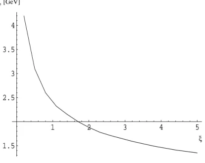
⁴

. (3.19) The first observation is that for all cases (i)–(iii) the large range of ξ values 0.2 ≤ ξ ≤ 5.0 there is a unique zero of f (ξ, Λ

b

) in Λ

b

. Second, the function Λ

b

(ξ) varies rather slowly (see Fig. 2). For example, for (i) a factor 25 in ξ implies a factor ∼ 3.1 in Λ

b

. Apart from the arguments of Section 2, this seems to give additional support to the definition (3.14).

1 2 3 4 5

1.5 2.5 3 3.5 4

Λ

ξ [GeV]

b

FIG. 2. The resolution scale Λ

b

as a function of ξ for the case (i).

Naturally, the formation scale of a Higgs condensate roughly coincides with the value of this condensate. We will use this fact in Section 4 to argue that Abelian projection is dynamical for resolutions ≤ Λ

b

. Resorting to ξ ∼ 1

⁴

, we have

(i) : Λ

b

(ξ ∼ 1) ∼ 2.4 GeV ; (ii) : Λ

b

(ξ ∼ 1) ∼ 3.1 GeV ; (iii) : Λ

b

(ξ ∼ 1) ∼ 4.2 GeV . (3.20) The most realistic case (i) corresponds to a condensation scale which is much higher than perturbatively determined scales Λ

QCD

which, depending on the number of active quark flavors and the renormalization scheme, range between 200–500 MeV. It is tempting to extrapolate to more realistic, that is, smaller quark masses. However, since N

F

= 4 and equal quark masses were assumed we feel that the uncertainty of such an extrapolation is too high for a conclusive statement. Hopefully, the results of more realistic lattice data simulations will soon become available. From (i) and (ii) in (3.20) it is clear that even at small quark mass m

q

the condensation scale Λ

b

depends rather strongly on it.

If the condensation scale Λ

b

in realistic QCD is higher than 1 GeV one would expect the standard operator product expansion (OPE) used in QCD sum rules [15] to be affected. At this scale one usually evaluates QCD sum rules [15]. There, the power corrections to a gauge invariant current correlator, introduced via the vacuum average of

4

This corresponds to the demand that Higgs condensation is described by a single scale Λ

b

.

(7)

the corresponding OPE, start at dimension four. This is a consequence of the perturbative calculation of Wilson coefficients. If there is a condensation of a Higgs field at the typical sum rule scale, as it is suggested by the above, the description of the non-perturbative QCD vacuum solely in terms of averages over local operators constructed from fundamental fields may not be sufficient since a composite scalar φ creates power corrections ∼ h φ

^a

φ

^a

i /Q

²

. In other words, the separation of nonlocal, potentially non-perturbative short distance effects into perturbatively calculated Wilson coefficients, which yield logarithmic factors

⁵

, is then not guaranteed to lead to an adequate discription at resolution Q ∼ 1 GeV. In refs. [18] and [19] power corrections due the short distance dynamics of small-size strings and instantons, respectively, have been argued to exist. In ref. [16] the introduction of Q

⁻²

power corrections due to non-perturbative short-distance effects was based on phenomenological grounds using the concept of a tachyonic gluon mass λ. It was found that a value as high as | λ | = 0.7 GeV is compatible with phenomenology in a variety of channels (ρ, π, scalar gluonium). Another approach to a short-distance dimension-two condensate in QCD defined in terms of fundamental fields has been proposed in refs. [17]. On the other hand, it was shown in ref. [16] that the ad hoc subtraction of the Landau pole in the running coupling α

s

(Q

²

) leads to a soft power correction ∼ Λ

²_QCD

/Q

²

. Attempts to develop a phenomenology of these long distance, power-two corrections were reported in refs. [20]. It is stressed at this point that the formation of a Higgs condensate at resolution Λ

b

freezes the perturbative running of the coupling to the value at this scale. So in the context of the present work there is a more profound alteration of the running of the coupling than a simple subtraction of the Landau pole.

4. HOW MAGNETIC MONOPOLES MAY FORM AND CONDENSE

Based on the above in this section we try to understand how the dual Meissner effect may be realized. In order to make the discussion simple we first consider pure SU(2) gluodynamics. Generalizations to SU(3) are straightforward.

Taking it as a fact that the vacuum below resolution Λ

b

is characterized by the dynamics of a Higgs field φ

^a

and a field α

µ

, which is pure gauge, one may construct a Georgi-Glashow like model with the curvature term for the gauge field missing:

L

vac

= 1

2 D

µ

φ

^a

D

µ

φ

^a

− V (φ

^a

φ

^a

) . (4.21)

Thereby, D

µ

φ

^a

≡ ∂ ˜

µ

φ

^a

− igε

^abc

α

^b_µ

φ

^c

, and V is some gauge invariant potential. Note that the connection α

µ

in this section is defined according to the perturbative convention, that is, one obtains α

µ

used here by multiplying α

µ

of Section 2 with i/g. In the background of α

µ

-fluctuations close to zero the apparent formation of a scalar condensate at resolution Λ

b

proceeds from condensation seeds. With these seeds present the growth of (3-dimensional) bubbles of constant Higgs field (constant color direction and modulus) sets in. Thereby, the color orientation inside a particular bubble is unrelated to that in the neighbouring bubble. Eventually, bubble edges collide. The probability that the Higgs directions of neighbouring bubbles coincide is exactly zero. Consequently, there are ”discontinuities” of the color orientation of the Higgs field over length scales of the order of the resolution Λ

⁻_b¹

across the bubble boundary.

From the kinetic part of (4.21) we have finite and positive energy density ε along the boundaries. This can most easily be seen as follows: Imposing the unitary gauge φ

^a

= | φ | δ

^3a

globally, one can shift the ”discontinuity” of the Higgs direction into a ”discontinuity” of the field α

µ6

. Without restriction of generality we assume that the boundary between two neighbouring bubbles A and B lies in the x

1

, x

2

-plane and that the Higgs field in A already is φ

^a

= | φ | δ

^3a

. The gauge transformation Ω reaching the global gauge φ

^a

= | φ | δ

^3a

in the vicinity of the boundary is given as

Ω = θ

Λ_b

( − x

3

)1 + θ

Λ_b

(x

3

)U

B

, U

B

≡ in

κ

τ

_κ^±

, (4.22) where τ

^±

= ( ~t/2, ∓ i 1 ), the components of n (n

κ

n

κ

= 1, κ = 1, 2, 3, 4) can be determined from the direction of the Higgs field in B, and θ

Λb

denotes a softened theta function for resolution Λ

b

5

Note, however, that the summation of certain perturbative diagrams leads to ambiguities (UV renormalons) which formally cause dimension two power corrections [14].

6

Within the collision zone the homogenity of the fields α

µ

and φ is destroyed. The contributions of undegenerated loops

should become important, and α

µ

is lifted from zero to a nonvanishing pure gauge configuration.

(8)

θ

Λ_b

(x

3

) ≡ θ(x

3

+ Λ

⁻_b¹

/2) θ( − x

3

+ Λ

⁻_b¹

/2) Λ

b

x

3

+ θ(x

3

− Λ

⁻_b¹

/2) . (4.23) The corresponding δ

Λb

function can be obtained from θ

Λb

by differentiation and omission of terms which contain ordinary delta functions as factors. Using (4.22), (4.23) and the fact that α

µ

is pure gauge, one obtains

ε = 1

2 g

²

| φ |

²

n α

¹_µ

2

+ α

²_µ

2

o

= 1

2 | φ |

²

(δ

Λb

)

²

n

²₁

+ n

²₂

= 2Λ

⁴_b

n

²₁

+ n

²₂

, ( − Λ

⁻_b¹

/2 ≤ x

3

≤ Λ

⁻_b¹

/2) , (4.24) where in the last line we have set the Higgs field modulus equal to the scale Λ

b

. Note that n

3

(or n

4

) is cyclic in (4.24) which signals the residual U(1) symmetry.

The vacuum manifold of the theory is the coset space M = SU (2)/U (1). It has the topology of a 2-sphere, and therefore it is simply connected. Two points can always be continuously connected, and hence there is no topological stabilization of the boundary between two domains. This means that localized energy density along the boundary at the time of collision can flow apart [21]. However, this happens due to approaching Higgs directions in a vicinity of the collision zone. At another boundary of the bubble, say, A the same process occurs but there with the Higgs field pointing in a different direction. After some time this implies localization of positive energy along a new domain boundary.

Now the positive energy along the domain boundaries must be countered by negative energy inside the domains to yield a vanishing action of the configuration. Negative energy is plausible since the formation of a Higgs condensate goes with a reduction of entropy density. This difference in energy density between the vacuum resolved at long and short distances was already incorporated in the bag models of hadrons [22] by means of the bag constant B.

Recall that the introduction of B is necessary to cure the non-conservation of bag four-momentum which is due to the violation of translational invariance by the bag boundary. We will soon argue that the presence of negative energy inside the domains, represented by a weakly varying Higgs condensate, also enforces a restoration of the (classical) translational and gauge symmetry at lower resolution.

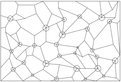
FIG. 3. A potential snapshot for a spatial slice of the YM vacuum at resolution Λ

b

. The solid lines indicate domain boundaries. Regions of potential monopole formation are encircled.

So far we only considered the boundary between two domains. Regions of exceptionally high, positive energy and

therefore exceptionally high instability of the Higgs condensate are those where several domains come together. They

can be string-like (3 domains meet along one edge) or point-like (generically 4 domains meet). As in the case of two

colliding domains strings are not stable topologically since any closed curve on M can be continuously deformed to a

point [21]. In the case of four or more domains coming together one cannot shrink the corresponding surface in M

to a point (the second homotopy group π

2

(M ) is non-trivial). So the cores of these regions are topologically stable

[21] and are characterized by a vanishing Higgs condensate. The more walls come together in a small region the more

profound the destruction of the Higgs condensate in that region is. The entire gauge group is restored there, and we

(9)

have magnetic monopoles or antimonopoles [23]

⁷

. In Fig. 2 a snapshot of a spatial slice of the domain structure of the vacuum at resolution Λ

b

is depicted.

An immediate consequence of the formation of magnetic monopoles and antimonopoles has been pointed out in the work of ref. [24]. There, it was argued that static, zero magnetic charge configurations such as the superposition of a ’t Hooft/Polyakov monopole and an antimonopole induce a nonvanishing spectral density of normalizable zero modes in the representation of the massless fermionic propagator in this background. According to [24] this implies a flavor independent breaking of chiral symmetry. This is in contrast to chiral symmetry breaking due to the instanton.

Moreover, the nonvanishing magnetic charge density is essential for the proliferation of the axial U(1) anomaly which prohibits the corresponding massless meson in the spectrum [24]. So already at resolution Λ

b

, which is much higher than the confinement scale, chiral symmetry breaking and the effects of the axial U(1) anomaly set in.

What about the condensation of monopoles? From the above it is clear that the average core sizes R of the (anti)monopoles are larger than Λ

⁻_b¹

which is comparable to the width of the domain boundaries. Furthermore, the long-range gauge field of the (anti)monopoles and the weak variation of the Higgs condensate inside the domains imply that these fields survive a grain coarsing to lower resolution. This is not the case for the domain boundaries.

As the resolution is tuned down the walls apparently cease to exist. To keep the configuration at vanishing action in this process the domains must shrink. At a critical resolution Λ

⁻_c¹

< R the walls vanish entirely, but not yet the cores of the monopoles. The only way to keep the action approximately at zero is a situation where the cores are arbitrarily close to one another to produce a vanishing energy density in the vacuum. This must be interpreted as the condensation of magnetic charges. Since monopoles are reduced to their cores they then can be considered massless. The relevant configurations at resolution ≤ Λ

c

are translationally invariant, and the gauge symmetry is restored everywhere since the Higgs field vanishes globally. Phenomenologically, one expects Λ

c

∼ Λ

QCD

∼ 0.3 GeV.

So, in agreement with a statement by Polyakov [25], the phenomenon of quark confinement goes together with the restoration of an apparently broken gauge symmetry.

To conclude this section let us remark on the relation between Abelian projection and the above picture in QCD.

So far we have only considered the vacuum fields of the (anti)monopoles far away from a core or inside a core. At intermediate distance from the core the constraint of nonvanishing curvature for the gauge field might be slightly violated, and gauge field fluctuations may propagate. Moreover, the presence of dynamical quarks also causes the curvature to be nonvanishing as was pointed out in the last section. In the following we speculate that Λ

b

∼ 1 GeV in QCD. It will be clear that qualitative implications do not depend on the exact value of Λ

b

.

In unitary gauge, φ

^a

=

^√¹₂

(δ

^3a

+ δ

^8a

) | φ | , off-diagonal gluons aquire a mass m

W

= g(Λ

b

) | φ | ∼ p

4πα

s

(Λ

b

)Λ

b

. (4.25)

Thereby, the running of α

s

is frozen at the value α

s

(Λ

b

) for resolution lower than Λ

b

. Diagonal gluons (photons) remain massless. Taking α

s

(Λ

b

= 1GeV) = 0.4

⁸

, one obtains m

W

= 2.24 GeV. So at resolution ≤ 1 GeV the dynamics of propagating gluons is Abelian to a very high degree. Moreover, photons are Debye-screened on distances comparable to the average monopole separation. At resolutions ∼ Λ

c

this distance vanishes and the (anti)monopoles become massless, so photons do not propagate at all. To estimate the mass of the two neutral Higgs particles let us assume that the dynamics of domain creation is goverened by a standard Higgs potential

V (φ

^a

φ

^a

) = β(φ

^a

φ

^a

− Λ

²_b

)

²

− γ . (4.26) To fix the parameters β, γ we impose

V (0) = 0 , V (Λ

b

, Λ

b

) = − B , (4.27)

where B is the bag constant. This gives β = B/(2Λ

⁴_b

) and γ = B. Moreover, the mass of the neutral scalars is m

H

= 2 √

B/Λ

b

. In ref. [27] the bag constant B ∼ 0.02 GeV

⁴

was determined from first principles of the bag

7

The properties (2.11) of the gauge field α

µ

far away from the cores are satisfied asymptotically also by the classical gauge field of the ’t Hooft/Polyakov (anti)monopole [23].

8

This value stems from a determination in the MS scheme with four-loop evolution and three-loop matching at the flavor

thresholds [26].

(10)

model and by using the QCD trace anomaly. We obtain m

H

∼ 280 MeV. According to this rough estimate, from a kinematical point of view these neutral scalars can be excited and propagate. However, they must be radiated off massive, highly virtual gluons which makes their appearance very unlikely. Nevertheless, it is tempting to speculate on the potential contribution of neutral Higgs excitations to the dark matter content of the universe. This issue will not be investigated further here.

5. SUMMARY AND CONCLUSIONS

Let us summarize the results of this work: Inspired by general renormalization group arguments [8] and the recently advocated expressibility of Abelian gauge fixed gluodynamics in terms of a Georgi-Glashow-like model [6] we have used Polyakov’s ideas [9] about chiral fields on the loop to define the corresponding vacuum fields in terms of fundamental fields in a nonlocal way. Appealing to lattice information on the gauge invariant field strength correlator [7,11,12], the resolution Λ

b

at which Higgs condensation can be observed in the vacuum was estimated for theories with and without dynamical fermions. It turned out that the values of Λ

b

are much larger than the perturbatively determined scales Λ

QCD

of the respective theories. This may have implications on the evaluation of OPE vacuum averages in the framework of QCD sum rules. Conventionally, Wilson coefficients, which carry nonlocal information on the scale of the external momentum probing the vacuum (usually ∼ 1 GeV), are calculated perturbatively. Our results seem to indicate, however, that the vacuum behaves highly non-perturbatively at this resolution already. Hence, the validity of a perturbative expansion of Wilson coefficients is questionable. This was stated in a similar way already in ref. [7].

Subsequently, it was argued that the randomness of the Higgs condensation implies the formation of domains which are bounded by positive energy walls. These walls are not stable and subject to constant rearrangement. For the action to remain zero it is necessary to have negative energy inside the domains. At locations where four or more domains meet the Higgs condensate is destroyed, and one has (topologically) stable magnetic (anti)monopoles. Together with the results of ref. [24] this implies that the onset of chiral symmetry breaking and the proliferation of the axial U(1) anomaly happens at the large resolution Λ

b

already. Describing the vacuum at resolution Λ ≤ Λ

b

in terms of a chiral gauge field and a Higgs field, the condensation of (anti)monopoles at Λ

c

< Λ

b

is a consequence of the weakly varying Higgs condensate, the long-range vector field of the (anti)monopole, and the fact that the width of the domain walls is smaller than the size of the cores of (anti)monopoles. Potentially propagating gluonic excitations were shown to be Abelian in nature. At resolution Λ

c

these excitation are completely Debye-screened due to the masslessness and the vanishing distance between (anti)monopoles. At higher resolutions there is a finite screening length comparable to the average distance between (anti)monopoles. On the other hand, the propagation of neutral Higgs excitations over large distances can not be excluded. However, the excitation of such particles seems to be extremely unlikely.

Further quantitative investigations are needed to decide whether these Higgs particles can contribute to the dark matter content of the universe in a sizable way.

NOTE ADDED

After completion of this work the author has become aware of a potential identification of the field φ/Λ

b

with the field ˆ n used in the nonlinear sigma model approach of Refs. [28]. The author would like to thank L. D. Faddeev for the corresponding remark.

ACKNOWLEDGMENTS

The author would like to thank the following people for useful conversations and discussions: O. Grandjean, F.

V. Gubarev, A. Hoang, B. P¨ otter, M. I. Polikarpov, G. Schierholz, L. Stodolsky, P. van Baal, P. Weisz, and V. I.

Zakharov. The author is indebted to V. I. Zakharov for a critical reading of the manuscript and the hinting on useful

literature.

(11)

[1] H. Fritzsch, M. Gell-Mann, and H. Leutwyler, Phys. Lett. B 47 , 365 (1973).

D. J. Gross and F. Wilczek, Phys. Rev. D 8 , 3633 (1973).

H. D. Politzer, Phys. Rev. Lett. 30 , 1346 (1973).

[2] S. Mandelstam, Phys. Rep. C 23 , 245 (1976).

G. ’t Hooft, Nucl. Phys. B 190 , 455 (1981).

[3] G. ’t Hooft, Nucl. Phys. B 190 , 455 (1981)

[4] R. C. Brower, K. N. Orginos, and C.-I. Tan, Phys. Rev. D 55 , 6313 (1997).

F. Bruckmann, T. Heinzl, T. Vekua, A. Wipf, Nucl. Phys. B 593 , 545 (2001).

R. Hofmann, hep-ph/0101317.

[5] H. Kleinert, Lett. Nuov. Cim. 34 , 209 (1982).

[6] P. Suranyi, hep-lat/0102009

[7] H. G. Dosch, Phys. Lett. B 190 , 177 (1987).

H. G. Dosch and Yu. A. Simonov, Phys. Lett. B 205 , 339 (1988).

[8] K. G. Wilson and J. Kogut, Phys. Rept. 12 , 75 (1974).

[9] A. M. Polyakov, Nucl. Phys. B 164 , 189 (1980)

[10] A. E. Dorokhov, S. V. Esaibegian, A. E. Maximov, and S. V. Mikhailov, Eur. Phys. J. C 13 , 331 (2000), hep-ph/9903450 [11] M. D’Elia, A. Di Giacomo, and E. Meggiolaro, Phys. Lett. B 408 , 315 (1997).