Evaluation of NorESM-OC (versions 1 and 1.2), the ocean

(1)

www.geosci-model-dev.net/9/2589/2016/

doi:10.5194/gmd-9-2589-2016

Evaluation of NorESM-OC (versions 1 and 1.2), the ocean

carbon-cycle stand-alone configuration of the Norwegian Earth System Model (NorESM1)

Jörg Schwinger¹, Nadine Goris¹, Jerry F. Tjiputra¹, Iris Kriest², Mats Bentsen¹, Ingo Bethke¹, Mehmet Ilicak¹, Karen M. Assmann^1,a, and Christoph Heinze^3,1

1Uni Research Climate, Bjerknes Centre for Climate Research, Bergen, Norway

2GEOMAR Helmholtz-Zentrum für Ozeanforschung, Kiel, Germany

3Geophysical Institute, University of Bergen, Bjerknes Centre for Climate Research, Bergen, Norway

anow at: Department of Marine Sciences, University of Gothenburg, Gothenburg, Sweden Correspondence to:Jörg Schwinger (jorg.schwinger@uni.no)

Received: 24 November 2015 – Published in Geosci. Model Dev. Discuss.: 15 January 2016 Revised: 8 June 2016 – Accepted: 4 July 2016 – Published: 2 August 2016

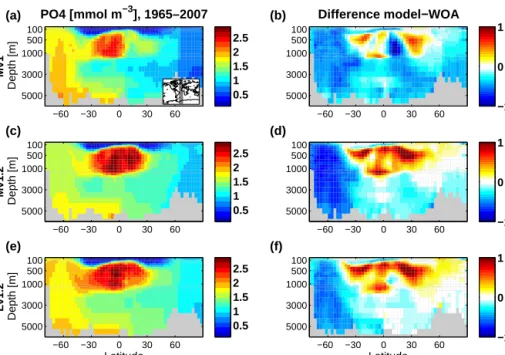
Abstract.Idealised and hindcast simulations performed with the stand-alone ocean carbon-cycle configuration of the Nor- wegian Earth System Model (NorESM-OC) are described and evaluated. We present simulation results of three different model configurations (two different model versions at different grid resolutions) using two different atmospheric forcing data sets. Model version NorESM-OC1 corresponds to the version that is included in the NorESM-ME1 fully coupled model, which participated in CMIP5. The main update between NorESM-OC1 and NorESM-OC1.2 is the addition of two new options for the treatment of sinking particles. We find that using a constant sinking speed, which has been the standard in NorESM’s ocean carbon cycle module HAMOCC (HAMburg Ocean Carbon Cycle model), does not transport enough particulate organic carbon (POC) into the deep ocean below approximately 2000 m depth. The two newly implemented parameterisations, a particle aggregation scheme with prognostic sinking speed, and a simpler scheme that uses a linear increase in the sinking speed with depth, provide better agreement with observed POC fluxes. Ad- ditionally, reduced deep ocean biases of oxygen and remineralised phosphate indicate a better performance of the new parameterisations. For model version 1.2, a re-tuning of the ecosystem parameterisation has been performed, which (i) reduces previously too high primary production at high latitudes, (ii) consequently improves model results for surface nutrients, and (iii) reduces alkalinity and dissolved inor-

ganic carbon biases at low latitudes. We use hindcast simulations with prescribed observed and constant (pre-industrial) atmospheric CO2concentrations to derive the past and contemporary ocean carbon sink. For the period 1990–1999 we find an average ocean carbon uptake ranging from 2.01 to 2.58 Pg C yr⁻¹depending on model version, grid resolution, and atmospheric forcing data set.

1 Introduction

Earth system models (ESMs) have been developed to take into account feedbacks between the physical climate and biogeochemical processes in projections of climate change (Bretherton, 1985; Flato, 2011). However, due to the com- plexity of feedback processes, it can prove useful to run one or several submodels of an ESM independently by using prescribed data at the boundary between submodel domains, e.g.

by using prescribed atmospheric conditions at the air–sea boundary to force the ocean and ice models of an ESM. Such

“stand-alone” model configurations are useful for conducting idealised experiments, for performing hindcast simulations in which boundary conditions reflect the observed variability and trends, or for saving computer time in cases where certain feedbacks are not expected to be important. Idealised experiments include set-ups where (purposefully manipulated) atmospheric output from fully coupled ESM runs is used to

(2)

force the stand-alone configuration of the same or another model.

Here, we describe and evaluate the stand-alone ocean carbon-cycle configuration of the Norwegian Earth System Model (NorESM-OC). Norwegian Earth System Model version 1 (NorESM1, Bentsen et al., 2013; Tjiputra et al., 2013) is derived from Community Earth System Model version 1 (CESM1, Gent et al., 2011; Lindsay et al., 2014), using the same sea-ice and land models as well as the same coupler but a modified atmospheric model (CAM4-Oslo, Kirkevåg et al., 2013) and a different ocean model. NorESM’s physical ocean component originates from the Miami Isopyc- nic Coordinate Ocean Model (MICOM; Bleck and Smith, 1990; Bleck et al., 1992), but has been updated with modified numerics and physics as described in Bentsen et al.

(2013). This model has been extended by Assmann et al.

(2010) to include HAMburg Ocean Carbon Cycle model version 5.1 (HAMOCC5.1, Maier-Reimer, 1993; Maier-Reimer et al., 2005). In the NorESM-OC configuration, MICOM- HAMOCC is coupled to CESM’s sea-ice model version 4 (CICE4, Holland et al., 2012) and a “data atmosphere” which provides atmospheric forcing fields to the ocean and sea-ice components.

The NorESM-OC model configuration allows us to study the global ocean carbon cycle and related biogeochemical cycles (phosphorus, nitrogen, silicate, iron, and oxygen) in idealised or hindcast simulations. We pursue two main ob- jectives with this set-up. First, it provides a simplified and computationally (relatively) inexpensive framework for the implementation and testing of new or updated model parameterisations. For example, we present the implementation and evaluation of new parameterisations for the sinking of particulate organic carbon (POC) in this work. In a fully coupled model set-up, atmospheric CO₂concentration is sensitive to the parameterisation of the biological pump (e.g. Marinov et al., 2006; Kwon et al., 2009), and eventually we aim to evaluate this sensitivity and associated feedbacks in the fully coupled version of NorESM. It is convenient, however, to perform a first evaluation without any feedback between biogeochemistry and physical climate (i.e. ocean circulation is unchanged in all test cases).

Second, hindcast simulations can provide insight into the response of biogeochemical cycles to observed variability and trends in atmospheric forcing. Of particular interest is the estimation of past and contemporary anthropogenic carbon uptake by the oceans using meteorological reanalysis data to force the ocean model. Such information is needed to better constrain the Earth system’s contemporary carbon budget, an effort undertaken by e.g. the Global Carbon Project (GCP, Le Quéré et al., 2015). Hindcast simulations performed with a first version of this model configuration (NorESM-OC1) contributed to the annual update of this carbon budget for the years 2011 to 2013. NorESM-OC1 corresponds to the version included in the fully coupled NorESM1-ME that is described in Tjiputra et al. (2013) and that participated

in phase 5 of the Coupled Model Intercomparison Project (CMIP5, Taylor et al., 2012).

Although NorESM-OC is computationally less expensive than the fully coupled NorESM, computational constraints limit the timescale for which the model can be applied to a few hundred to 1000 years on current hardware. We note that this limitation is mainly due to the physical ocean model and the costly transport of tracers. By using an efficient offline method (e.g. Khatiwala et al., 2005; Kriest et al., 2012), it would be possible to apply HAMOCC on timescales at least 1 order of magnitude longer, as long as all relevant external inputs are provided (e.g. fluxes due to continental weathering). Similar versions of HAMOCC have been applied on timescales of 50 000 years (e.g. Heinze et al., 2003, who use an offline set-up with annually averaged ocean circulation fields).

In this paper we describe NorESM-OC1 next to an updated version of the model system (NorESM-OC1.2), which is configured on a numerically more efficient grid at either 1^◦ or 2^◦ nominal resolution, includes additional parameterisations for the sinking of POC, and features several updates and improvements as described in Sect. 2. Spin-up followed by hindcast simulations forced by two slightly different forcing data sets have been performed for the different model versions and configurations. We evaluate the model results against available observation-based climatolo- gies (Sects. 3.1 to 3.3), and we calculate ocean carbon sink estimates and anthropogenic carbon storage (Sect. 3.4). The newly implemented particle sinking schemes are evaluated using observation-based estimates of global POC fluxes and of remineralisation as well as sediment trap data (Sect. 3.5).

We conclude by discussing the current status of the model system and lines of further development.

2 Model description and configuration

The components of NorESM discussed here have been described and evaluated in papers published previously in this special issue (Bentsen et al., 2013; Tjiputra et al., 2013) and elsewhere (Danabasoglu et al., 2014; Griffies et al., 2014;

Downes et al., 2015; Farneti et al., 2015). Therefore, we only give a brief description of the NorESM-OC model components and focus on documenting the specific model configurations and the updates made for NorESM-OC1.2.

2.1 The MICOM physical ocean model

The main benefit of an isopycnal model is the good con- trol on the diapycnal mixing (less numerical diffusion across isopycnic surfaces) that helps to preserve water masses during long model integrations. This is of particular interest for a coupled physical–biogeochemical model, since sharp gra- dients in tracer concentrations between water masses (e.g. in the thermocline region) can potentially be better represented

(3)

by the model. The isopycnic framework provides a smooth representation of bottom topography, and therefore overflow of water masses is modelled without numerical obstacles (although mixing at steep slopes must be parameterised care- fully).

As mentioned above, the model is based on MICOM as described by Bleck and Smith (1990) and Bleck et al.

(1992). Key aspects retained from this model version are a mass-conserving formulation (non-Boussinesq), Arakawa C-grid discretisation, leap-frog and forward–backward time- stepping for the baroclinic and barotropic modes, respectively, and a potential vorticity/enstrophy conserving scheme for the momentum equation. Differently from the original MICOM, we use the incremental remapping algorithm of Dukowicz and Baumgardner (2000) for transport of layer thickness, potential temperature, salinity, and tracers. The second-order accurate algorithm is expressed in flux form and thus conserves mass by construction. Furthermore, it guarantees monotonicity of tracers (i.e. the scheme does not create new minima or maxima) for any velocity field.

Originally, MICOM had a single bulk surface mixed layer, while in NorESM the mixed layer is divided into two model layers with freely evolving density and equal thickness when the mixed layer is shallower than 20 m. The uppermost layer is limited to 10 m when the mixed layer is deeper than 20 m.

The main reason for this is to allow for a faster ocean surface response to surface fluxes. We achieve reduced mixed layer depth biases (compared to the original MICOM) by using a turbulent kinetic energy (TKE) model based on Ober- huber (1993), extended with a parameterisation of mixed layer restratification by submesoscale eddies (Fox-Kemper et al., 2008). To improve the representation of water masses in weakly stratified high-latitude haloclines, the static stabil- ity of the uppermost layers is measured by in situ density jumps across layer interfaces, thus allowing for layers that are unstable with respect to potential density referenced at 2000 dbar to exist. The diagnostic version of the eddy clo- sure of Eden and Greatbatch (2008) as implemented by Eden et al. (2009) is used to parameterise the thickness and isopycnal eddy diffusivity. Further, to reduce sea surface salinity and stratification biases at high latitudes, salt released during freezing of sea ice can be distributed below the mixed layer.

The ocean component exchanges no mass with the other components of NorESM. Thus, freshwater fluxes are con- verted to virtual salt and tracer fluxes before they are applied to the ocean.

2.2 The CICE sea-ice model

NorESM-OC employs the CESM sea-ice component, which is based on version 4 of the Los Alamos National Laboratory sea-ice model (CICE4, Hunke and Lipscomb, 2008). Impor- tant modifications of this model that are utilised in CESM and NorESM1 are the delta-Eddington short-wave radiation transfer as well as melt pond and aerosol parameterisations,

all described by Holland et al. (2012). The sea-ice model shares the same horizontal grid with the ocean component of NorESM.

2.3 The HAMOCC5.1 marine biogeochemistry model The HAMburg Ocean Carbon Cycle (HAMOCC) model is based on the original work of Maier-Reimer (1993) and subsequent refinements (Maier-Reimer et al., 2005). The model simulates the marine biogeochemical cycles of carbon, nitrogen, phosphorus, silicate, iron, and oxygen, including the fluxes of these elements across the air–sea interface. HAMOCC5.1 was coupled with the isopycnic MICOM model by Assmann et al. (2010). We describe a version of the code that evolved from this point and note that the original model has also been further developed by the biogeochemistry group at the Max Planck Institute in Hamburg (Ilyina et al., 2013). The model described by Assmann et al. (2010) was the starting point for the development of the ocean biogeochemistry component of NorESM1. Main differences between this model and NorESM-OC1 are updates of mixed layer and eddy diffusivity parameterisations, the use of CICE as an ice model, and the details of atmospheric forcing, which followed Bentsen and Drange (2000), whereas NorESM-OC uses the approach of Large and Yeager (2004). The version of HAMOCC employed by Assmann et al. (2010) is very similar to the one in NorESM-OC1, with the notable difference of an update of the carbon chemistry scheme (see below).

The HAMOCC code is embedded in MICOM, and hence runs at the same spatial and temporal resolution as the ocean model. The model has 19 prognostic tracers (Table 1), all of which are advected and diffused with the ocean circulation provided by MICOM. Two additional tracers are needed if the particle aggregation scheme (prognostic sinking speed;

see Sect. 2.3.3) is switched on. There are also three “preformed” tracers for oxygen, phosphate, and alkalinity, which are set to the corresponding concentration values in the surface mixed layer at each time step, and are otherwise pas- sively advected. Preformed tracers have been introduced in version 1.2 to enhance the diagnostic capabilities of the model.

When HAMOCC was implemented as the biogeochemistry module of MICOM, the biogeochemical tracers were only defined at one of the two time levels of the leap-frog time-stepping scheme to increase computational efficiency (Assmann et al., 2010). To prevent amplification of numerical noise, the MICOM leap frog time-stepping includes a time-smoothing applied to the mid time level of temperature, salinity, and layer thickness fields at each time step, i.e. x_mid=w₁x_mid+w₂(x_old+x_new), withw₁=0.875 and w₂=0.0625. Since the physical fields undergo this time smoothing, but in NorESM-OC1 the biogeochemical tracers do not, there is an inconsistency between physical fields and biogeochemical tracers introduced by this simplification, which results in a non-conservation or tracer mass.

(4)

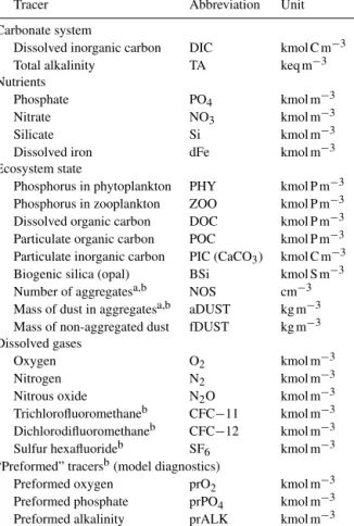
Table 1.Prognostic biogeochemical tracers in NorESM-OC.

Tracer Abbreviation Unit

Carbonate system

Dissolved inorganic carbon DIC kmol C m⁻³

Total alkalinity TA keq m⁻³

Nutrients

Phosphate PO₄ kmol m⁻³

Nitrate NO₃ kmol m⁻³

Silicate Si kmol m⁻³

Dissolved iron dFe kmol m⁻³

Ecosystem state

Phosphorus in phytoplankton PHY kmol P m⁻³ Phosphorus in zooplankton ZOO kmol P m⁻³ Dissolved organic carbon DOC kmol P m⁻³ Particulate organic carbon POC kmol P m⁻³ Particulate inorganic carbon PIC (CaCO₃) kmol C m⁻³ Biogenic silica (opal) BSi kmol S m⁻³ Number of aggregates^a,b NOS cm⁻³ Mass of dust in aggregates^a,b aDUST kg m⁻³ Mass of non-aggregated dust fDUST kg m⁻³ Dissolved gases

Oxygen O₂ kmol m⁻³

Nitrogen N2 kmol m⁻³

Nitrous oxide N₂O kmol m⁻³

Trichlorofluoromethane^b CFC−11 kmol m⁻³ Dichlorodifluoromethane^b CFC−12 kmol m⁻³ Sulfur hexafluoride^b SF₆ kmol m⁻³

“Preformed” tracers^b(model diagnostics)

Preformed oxygen prO₂ kmol m⁻³

Preformed phosphate prPO₄ kmol m⁻³ Preformed alkalinity prALK kmol m⁻³

aOnly if particle aggregation (prognostic sinking speed) is activated.

bAvailable as of version NorESM-OCv1.2.

This non-conservation is accounted for in model version 1 by a correction factor applied after the time-smoothing to the biogeochemical tracer fields. Although simulation results were not significantly affected on integration timescales of

≈1000 years, we decided to re-implement the tracer transport scheme to make it fully consistent with the physical fields in version 1.2 by defining the tracer fields on two time levels and applying the same time-smoothing procedure as for the physical fields. We anticipate that this im- provement will become important on integration timescales of 10 000 years or longer.

2.3.1 Air–sea gas exchange and inorganic carbon chemistry

HAMOCC calculates the exchange of various gases through the air–sea interface. This exchange is determined by three components: the gas solubility in seawater, the gas transfer rate, and the gradient of the gas partial pressure between the atmosphere and the ocean surface. The solubilities of O₂ and N₂ in seawater as functions of surface ocean temperature and salinity are taken from Weiss (1970), and solubilities of CO₂and N₂O from Weiss and Price (1980). Solu-

bilities of sulfur hexaflouride (SF6) and the two chlorofluo- rocarbons CFC-11 and CFC-12 are calculated according to Warner and Weiss (1985) and Bullister et al. (2002). The gas transfer rates are computed using the empirical relationship k=a U₁₀²(660/Sc)^1/2derived by Wanninkhof (1992), where U₁₀ is the surface wind speed at 10 m reference height and a is a gas-independent constant. The Schmidt numberScis the kinematic viscosity divided by the diffusivity of the respective gas component, and 660 is the Schmidt number of seawater at 20^◦C. Schmidt numbers for CO₂and CFCs have been taken from Wanninkhof (1992). Since the polynomial used there to fit the experimental data displays non-physical behaviour outside the validity range of the fit for tempera- tures>30^◦C (very small and negative Schmidt numbers), we use the re-fitted temperature dependence recommended by Gröger and Mikolajewicz (2011) in model version 1.2. We note that the updated air–sea gas exchange formulation provided by Wanninkhof (2014) also includes re-fitted Schmidt numbers, avoiding problems at high SST. The Schmidt number for O₂is taken from Keeling et al. (1998), and the same value is assumed also for N₂and N₂O. The model has no gas exchange through ice-covered surface areas of a grid cell, and for partly ice-covered grid cells the gas exchange flux is scaled to the ice-free fraction of the cell.

Compared to the original HAMOCC (Maier-Reimer et al., 2005) and to the version used by Assmann et al. (2010), our model includes a revised inorganic seawater carbon chemistry following Dickson et al. (2007). Total alkalinity (TA) is defined as including contributions of boric acid, phosphoric acid, hydrogen sulfate, hydrofluoric acid, and silicic acid, TA=[HCO⁻₃] +2[CO²⁻₃ ] + [B(OH)⁻₄] + [OH⁻]

+ [HPO²⁻₄ ] +2[PO³⁻₄ ] + [SiO(OH₃)⁻]

− [H⁺]−[HSO⁻₄]−[HF]−[H3PO4]. (1) We use an iterative carbonate alkalinity correction method (Follows et al., 2006; Munhoven, 2013) to calculate the oceanic partial pressure of CO₂(pCO₂) prognostically as a function of temperature, salinity, dissolved inorganic carbon (DIC), and TA. Using an initial guess for the hydrogen ion concentration[H⁺]₀, all non-carbonate contributions to TA are calculated according to Dickson et al. (2007) and added to or subtracted from Eq. (1) in order to obtain an initial guess for carbonate alkalinity CA₀ (CA = [HCO⁻₃] +2[CO²⁻₃ ]).

Given CA and DIC and the equilibrium constants of the carbonate systemK₁andK₂, the corresponding hydrogen ion concentration can be calculated:

[H⁺] = K1

2 CA (2)

DIC−CA+ q

(DIC−CA)²+4 CAK₂/K₁(2 DIC−CA)

.

The hydrogen ion concentration[H⁺]₁ thus obtained is used to re-iterate these calculations until convergence is

(5)

reached. Here, we use [H⁺]from the previous time step as an initial guess for the calculation of CA, and stop iterations once the relative change ([H⁺]_i+1− [H⁺]_i)/[H⁺]_i+1) becomes smaller than=5×10⁻⁵. Only at the first time step of integration do we use[H⁺]₀=10⁻⁸mol kg⁻¹. As pointed out by Follows et al. (2006), the changes in[H⁺]from one time step to the next are small, and one or a few iterations of this procedure usually suffice. The effect of pressure on the various dissociation constants is calculated according to Millero (1995).

2.3.2 Ecosystem model

HAMOCC5.1 employs an NPZD-type (nutrient, phytoplankton, zooplankton and detritus) ecosystem model, extended to include dissolved organic carbon (DOC). The ecosystem model was initially implemented by Six and Maier- Reimer (1996). The nutrient compartment is represented by three macronutrients (phosphate, nitrate, silicate) and one micronutrient (dissolved iron). A constant Redfield ratio of P :C: N:O₂ =1:122:16: −172 following Takahashi et al. (1985) is used. That is, the ratios of carbon to phosphorus and nitrogen to phosphorus in organic matter are R_C:_P=122 andR_N:P=16, respectively, andR_O₂:P=172 moles of oxygen are consumed during remineralisation of 1 mole of phosphorus.

The phytoplankton growth rateJ (I, T )follows the light- saturation curve formulation of Smith (1936):

J (I, T )= ασ I (z)f (T )

p(ασ I (z))²+f (T )², (3) with temperature dependence parameterised according to Eppley (1972), f (T )=µ_phy1.066^T. Here, α=0.02 is the initial slope of the photosynthesis vs. irradiance curve,σ= 0.4 is the fraction of photosynthetically active radiation, andµ_phy=0.6 d⁻¹. The available light is calculated based on incoming solar radiation prescribed through the atmospheric forcing (I₀) and attenuation through seawater (k_w) and chlorophyll (k_chl)

I (z)=I0e^−(k^w^+k^chl^Chl)z. (4) Chlorophyll (Chl) is calculated from phytoplankton mass assuming a constant carbon to chlorophyll ratioRC:Chl=60.

A disadvantage of an isopycnic model is the low vertical resolution in weakly stratified regions. The mixed layer in MICOM was represented by only one model layer in Ass- mann et al. (2010). For NorESM a second model layer has been added to improve the simulation of mixed layer processes. The top model layer varies in thickness between 5 and 10 m, while the second model layer represents the rest of the mixed layer. Consequently, for deep mixed layers, the second model layer will often have a vertical extent of 100 m and more, which still results in a rather poor resolution for the simulation of biological processes. We therefore decided to

re-implement Eq. (4) for NorESM-OC1.2 by calculating the average light availabilityI (instead of using the light availability at the centre of layers), which reads for layeri:

Ii=I0,i

1

(k_w+k_chlChl_i)1z_i

1−e^−(k^w^+k^chl^Chlⁱ^)1zⁱ . (5) In addition to light limitation, phytoplankton growth is co- limited by availability of phosphate, nitrate, and dissolved iron. The nutrient limitation is expressed through a Monod functionf_nut=X/(K+X), whereK is the half-saturation constant for nutrient uptake (K=4×10⁻⁸kmol P m⁻³), and X=min

PO₄, NO₃ R_N:P

, Fe R_Fe:P

. (6)

RN:P=16 andRFe:P=366×10⁻⁶are the (constant) nitrogen to phosphorus and iron to phosphorus ratios for organic matter used in the model. Aerial dust deposition to the surface ocean is prescribed based on Mahowald et al. (2006).

A fraction of the dust deposition (1 %) is assumed to be iron, and part of it is immediately dissolved and available for biological production. To mimic the process of complexation with ligands, iron concentration is relaxed towards a value of 0.6 µmol m⁻³when modelled iron is larger than this value.

We note that this parameterisation of the iron cycle is rather simplistic. The spatial pattern of iron in the surface mainly reflects the aeolian input and upwelling of iron in the South- ern Ocean. At depth, iron concentration is determined by ac- cumulation of remineralised iron and the assumed complexation. Therefore, the iron concentration approaches a constant value of 0.6 µmol m⁻³ at depths larger than approximately 700 m. We find that the resulting iron limitation in our model is rather weak, and given these limitations we will not focus on the iron cycle in this paper.

In nitrate-limited regions, i.e. if[NO₃]< R_N:P[PO₄], the model assumes nitrogen fixation by cyanobacteria in the surface layer. The distributions of calcium carbonate and biogenic silica export productions depend on the availability of silicic acid, since it is implicitly assumed that diatoms out- compete other phytoplankton species when the supply of silicic acid is sufficient. This is parameterised by assuming that a fraction[Si]/(KSi+[Si])of export production contains opal shells while the remaining fraction contains calcareous shells, whereKSi=1 mmol Si m⁻³is the half-saturation constant for silicate uptake (Martin-Jézéquel et al., 2000). Phyto- plankton loss is modelled by specific mortality and exudation rates as well as zooplankton consumption. DOC is produced by phytoplankton and zooplankton (through constant exudation and excretion rates) and is remineralised at a constant rate (whenever the required oxygen is available). The full set of differential equations defining the ecosystem can be found in Maier-Reimer et al. (2005).

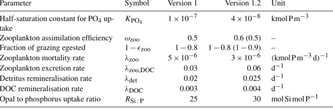
Between model versions 1 and 1.2 we performed a re- tuning of the ecosystem parameterisation (see Table 2 for old and new parameter values). The objective of this effort was

(6)

Table 2.Parameter values of the ecosystem parameterisation (see Maier-Reimer et al., 2005, for details) that have been changed between model versions 1 and 1.2. Parameter values in brackets have been used for the model runs with the non-standard sinking schemes (Sect. 3.5).

Parameter Symbol Version 1 Version 1.2 Unit

Half-saturation constant for PO₄uptake

K_PO₄ 1×10⁻⁷ 4×10⁻⁸ kmol P m⁻³ Zooplankton assimilation efficiency ωzoo 0.5 0.6 (0.5) –

Fraction of grazing egested 1−zoo 1−0.8 1−0.8 (1−0.9) –

Zooplankton mortality rate λzoo 5×10⁻⁶ 3×10⁻⁶ (kmol P m⁻³d)⁻¹

Zooplankton excretion rate λ_zoo,DOC 0.03 0.06 d⁻¹

Detritus remineralisation rate λ_det 0.02 0.025 d⁻¹

DOC remineralisation rate λ_DOC 0.003 0.004 d⁻¹

Opal to phosphorus uptake ratio R_{Si : P} 25 30 mol Si mol P⁻¹

to (i) reduce previously overestimated primary production at high latitudes, (ii) increase production in the low-latitude oligotrophic gyres, and (iii) reduce a low-latitude bias in alkalinity and DIC found in model version 1. The tuning was not based on an objective procedure, but relied on the au- thors’ experience and a series of “trial and error” simulations.

Points (i) and (ii) were addressed by increasing zooplankton abundance (decreasing zooplankton mortality λ_zoo and increasing zooplankton assimilation efficiencyω_zoo), which helps to limit primary production in the high-latitude “high- nutrient, low-chlorophyll” regions. Further, phytoplankton growth is stimulated mainly at low latitudes by reducing the half-saturation constantK_PO₄and by increasing available nutrients in the surface by slightly increasing the remineralisation of detritus and DOC. The alkalinity and related DIC biases (iii) were addressed by reducing the surface concentration of silicate in order to increase CaCO3production. This was done by increasing the opal to phosphorus uptake ratio RSi:P.

2.3.3 Particle export and sinking

The standard HAMOCC scheme for the treatment of sinking particles assumes a prescribed constant sinking speed for three classes of particles. Particulate organic carbon associated with dead phytoplankton and zooplankton is trans- ported vertically at 5 m d⁻¹. As POC sinks, it is remineralised at a constant rate and according to oxygen availability. When oxygen concentration falls below a thresh- old of 0.5 µmol L⁻¹, POC is remineralised by denitrification.

Without explicitly modelling this process, it is assumed that 2/3×RO₂:P≈115 moles of nitrate are consumed by deni- trifying bacteria to remineralise an amount of detritus corresponding to 1 mole of phosphate (i.e. it is assumed that the oxygen from 2 moles of nitrate substitutes 3 moles of oxygen during denitrification). Particulate inorganic carbon (calcium carbonate, PIC) and opal shells (biogenic silica) sink with a fixed speed of 30 m d⁻¹. Biogenic silica is decom- posed at depth with a constant dissolution rate, while the dissolution of calcium carbonate shells depends on the sat-

uration state with respect to CaCO3in the surrounding seawater. Non-remineralised particulate materials reaching the sea floor sediment undergo chemical reactions with the sediment pore waters and vertical advection within the sediment.

The 12-layer sediment model (Heinze et al., 1999; Maier- Reimer et al., 2005) is primarily relevant for long-term simulations (>1000 years). Nevertheless, the sediment model was activated for all simulations presented here. The current model version neither includes a parameterisation of weathering fluxes nor takes into account the influx of carbon and nutrients through continental discharge. The mate- rial lost to the sediments is therefore not replaced by some mechanism in the model configurations presented here. The model drift caused by these losses to the sediment is small on the timescales considered in this paper, particularly at the surface. Nevertheless, this simplification limits the applica- bility of NorESM-OC1 and 1.2 to timescales of the order of 1000 years. Input of DIC and nutrients in particulate and dissolved forms through rivers is currently implemented in NorESM.

In NorESM-OC1.2 we provide two alternative options for the treatment of particle sinking. First, a scheme which calculates the sinking speed as a linear function of depth as w_POC=min(w_min+a z, w_max)has been implemented. Here, w_min is the minimum sinking speed found atz=0, and a is a constant describing the increase in speed with depth.

The sinking speed can be limited by setting the parame- terwmax. We refer to this scheme as WLIN in the following text, and we usewmin=7 m d⁻¹,wmax=43 m d⁻¹, and a=40/2500 m d⁻¹m⁻¹in this study. Note that forwmin=0 and wmax= ∞, this parameterisation is equivalent to the widely used Martin-curve formulation (Martin et al., 1987;

Kriest and Oschlies, 2008).

The second new option is a scheme with variable (prognostic) sinking speed which is calculated according to a size distribution of sinking particles. Since an explicit representation of sinking particles through a large number of dis- crete size classes would not be feasible in a large-scale Earth system model due to computational constraints, we imple-

(7)

mented the particle aggregation and sinking scheme devised by Kriest and Evans (1999) and Kriest (2002) as a cost- effective alternative. This model (hereafter abbreviated as KR02) assumes that phytoplankton and detritus form sinking aggregates and that the size distribution of aggregates obeys a power-law formulation

n(d)=A d^−ε, l < d <∞, (7) wheredis the particle diameter, andAandεare parameters of the distribution. The lower bound of diametersl concep- tually corresponds to the size of a single cell. Large values of ε(a steeper slope of the distribution) correspond to a larger number of slow-sinking small particles. By integration over the size range froml to∞, the total number of aggregates (NOS) is obtained,

NOS=A

∞

Z

l

d^−εdd=A l^(1−ε)

(ε−1), (8)

provided that ε >1. The mass of an aggregate is described byCd^ζand, consequently, the total mass of aggregates reads M=A Cl

l^(1−ε)

(ε−1−ζ )=PHY+POC, (9) whereC_l=Cl^ζ is the mass of a single cell. If particles were spheres with constant density, then ζ =3. Since the mass of aggregates grows more slowly than the cube of their diameter, we adopt the value ζ =1.62 used in Kriest (2002).

Finally, it is assumed that the sinking speed of aggregates depends on the diameter according to w(d)=Bd^η, with wl=Bl^η being the sinking speed of a single cell. The total phytoplankton and detritus mass M=PHY+POC and the number of aggregates NOS are the prognostic variables of the KR02 scheme as implemented in HAMOCC. GivenM and NOS, the parametersandAof the particle size distribution can be determined, and from these the average sinking speeds for mass and numbers are obtained.

NOS is treated like other particulate tracers in the model;

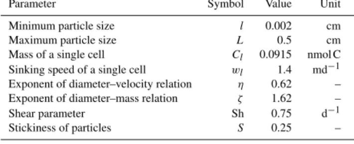
that is, NOS is advected and diffused by ocean circulation and treated in HAMOCC’s sinking scheme (see below) using the average sinking speed for particle numbers as given in Kriest (2002). Additionally, aggregation of particles de- creases NOS, while photosynthesis, egestion of fecal pellets, and zooplankton mortality increase NOS. The size distribution is affected by these processes as follows. Sinking re- moves preferentially the large particles and leaves behind the smaller ones, thereby steepening the slopeεof the size spectrum in surface layers. Aggregation “flattens” the slope of the size spectrum, because it reduces the number of particles but not mass. These processes are parameterised as in sce- nario pSAM of Kriest (2002), but with stickiness set to 0.25, the factor for shear collisions set to 0.75 d⁻¹, and a maximum particle size for size-dependent aggregation and sinking of 0.5 cm (see Table 3 for a summary of parameter values). We assume that all other biogeochemical processes do

Table 3.Parameter values adopted for the prognostic sinking speed scheme.

Parameter Symbol Value Unit

Minimum particle size l 0.002 cm

Maximum particle size L 0.5 cm

Mass of a single cell C_l 0.0915 nmol C Sinking speed of a single cell w_l 1.4 md⁻¹ Exponent of diameter–velocity relation η 0.62 – Exponent of diameter–mass relation ζ 1.62 –

Shear parameter Sh 0.75 d⁻¹

Stickiness of particles S 0.25 –

not impactε(e.g. photosynthesis increasesMand NOS pro- portionally, such that the slope of the size distribution is not affected), the exception being zooplankton mortality, which flattens the size spectrum through the addition of (large) zooplankton carcasses.

An implicit scheme is used to redistribute mass (and the number of particles in the case of KR02) through the water column:

C_i^t+dt=C_i^t+ dt 1z_i

wi−1C_i^t+dt₋₁ −wiC_i^t+dt

, (10)

where dt is the time-step length,1zi the thickness of layer i,Cstands for the concentration of POC, PIC, opal, or NOS, andw_i is the corresponding sinking speed at layer i. This scheme is used with prognostic or prescribed sinking speed options. Note that in the KR02 schemew is a function of time and would be evaluated at time levelt+dt in a fully implicit discretisation. This, however, is practically impossi- ble and we resort to the common simplification of evaluating wat the old time level (“lagging the coefficients”, Anderson, 1995) for the purpose of solving Eq. (10). We further note that PIC and opal are sinking at a fixed prescribed rate of 30 md⁻¹if the standard or WLIN scheme is used, but are assumed to sink as a component of the phytoplankton–detritus aggregates in the KR02 scheme (i.e. at the prognostic sinking speed calculated by the scheme). For a more detailed discussion of the KR02 scheme in comparison to the assumption of constant or linearly increasing sinking speed, we refer the reader to Kriest and Oschlies (2008).

2.4 Model configuration

We discuss three different model grid configurations, one for NorESM-OC1, which runs on a displaced pole grid with 1.125^◦ nominal resolution and with grid singularities over Antarctica and Greenland. NorESM-OC1.2 has been set up on a numerically more efficient tripolar grid at 1 and 2^◦ nominal resolution. The tripolar grid has its singularities at the South Pole, in Canada, and in Siberia. The nominal resolutions given here indicate the zonal resolution of the grid, while the latitudinal resolution is finer and variable. For the displaced pole grid of NorESM-OC1, the latitudinal grid spacing is 0.27^◦ at the Equator, gradually in-

(8)

creasing to 0.54^◦at high southern latitudes. The tripolar grid of NorESM-OC1.2 is optimised for isotropy of the grid at high latitudes, and the latitudinal spacing varies from 0.25^◦ (0.5^◦) at the Equator to 0.17^◦(0.35^◦) at high southern latitudes for the 1^◦(2^◦) nominal resolution. Note that over the Northern Hemisphere both grid types are distorted to accom- modate the displaced pole over Greenland or the dual-pole structure over Canada and Siberia. Due to the more evenly distributed grid spacing of the tripolar grid in the Northern Hemisphere, the time step can be increased from 1800 to 3200 s, and a time step of 5400 s can be used for the 2^◦configuration. We use the abbreviations Mv1, Mv1.2, and Lv1.2 for the three versions/configurations, where “M” and “L” refer to medium (1^◦) and low (2^◦) resolution, respectively, followed by the version number of the model. All variants of NorESM-OC discussed here are configured with 51 isopycnic layers referenced at 2000 dbar and potential densities ranging from 28.202 to 37.800 kg m⁻³. The reference pressure at 2000 dbar provides reasonable neutrality of model layers in large regions of the ocean (McDougall and Jackett, 2005).

2.4.1 Forcing

The atmospheric forcing required to run NorESM-OC com- prises air temperature, specific humidity and wind at 10 m reference height, as well as sea-level pressure, precipitation, and incident short-wave radiation fields. Two variants of the data sets developed for the Coordinated Ocean-ice Refer- ence Experiments (COREs, Griffies et al., 2009), the CORE normal-year forcing (CORE-NYF, Large and Yeager, 2004) and the CORE interannual forcing (CORE-IAF, Large and Yeager, 2009), can be used to provide the atmospheric forcing for NorESM-OC. Both data sets are based on the NCEP reanalysis (Kalnay et al., 1996) and a number of observational data sets. Corrections are applied to the NCEP surface air temperature, wind, and humidity to remove known biases, while precipitation and radiation fields are derived entirely from satellite observations (see Large and Yeager, 2004, 2009, for details). The near-surface atmospheric state has a 6-hourly frequency, while the radiation and precipitation fields are daily and monthly means, respectively. The normal-year forcing has been constructed to represent a climatological mean year with a smooth transition between the end and start of the year (Large and Yeager, 2004). This forcing can be applied repeatedly for as many years as needed to force an ocean model without imposing interannual variability or discontinuities. We use this forcing data set to spin up our model. The CORE-IAF consists of the corrected NCEP data for the years 1948–2009. Radiation and precipitation data sets are daily and monthly climatological means before 1984 and 1979, respectively, and vary interannually for the time period thereafter.

Since we wish to run hindcast simulations up to the present date, but the CORE-IAF only covers the years 1948 to 2009,

we devised an alternative data set, which is identical to the CORE-IAF for surface air temperature, wind, humidity, and density (i.e. the same corrections as for the CORE-IAF are applied to the NCEP reanalysis data), but the radiation and precipitation fields are taken from the NCEP reanalysis without any corrections. NCEP surface air temperature and specific humidity are re-referenced from 2 to 10 m reference height following the same procedure as used for the CORE forcings (S. Yeager, personal communication, 2012). We refer to this forcing data set as NCEP-C-IAF in the following text.

Continental freshwater discharge is based on the climatological annual mean data set described by Dai and Tren- berth (2002). It has been modified to include a 0.073 Sv con- tribution from Antarctica as estimated by Large and Yeager (2009). This freshwater discharge is distributed evenly along the coast of Antarctica as a liquid freshwater flux. All runoff fluxes are mapped to the ocean grid and smeared out over ocean grid cells within 300 km of each discharge point to account for unresolved mixing processes.

In order to stabilise the model solution, we apply salinity relaxation towards observed surface salinity with restoring timescales of 365 days (version 1) and 300 days (version 1.2) for a 50 m thick surface layer. The restoring is applied as a salt flux which is also present below sea ice. In model version 1.2, balancing of the global salinity relaxation flux was added as an option, which allows us to keep the global mean salinity constant over long integration times. That is, positive (negative) relaxation fluxes (where “positive” means a salt flux into the ocean) are decreased (increased) by a multiplicative factor if the global total of the relaxation flux is positive (negative). The somewhat shorter relaxation timescale applied in version 1.2 was chosen to approximately counter- act the weakening of the relaxation flux due to this balancing procedure. Another option introduced in version 1.2 is a weaker salinity relaxation over the Southern Ocean south of 55^◦S with a linear ramp between 40 and 55^◦S. This mea- sure can slightly improve the simulated Southern Ocean hy- drography and tracer distributions. Both new options have been activated for all simulations with model version 1.2 presented here, and a timescale of 1050 days has been used for SSS relaxation south of 55^◦S.

2.4.2 Initialisation and simulation set-up

The physical ocean model is initialised with zero velocities and the January mean temperature and salinity fields from the Polar Science Center Hydrographic Climatology (PHC) 3.0 (Steele et al., 2001). Initial concentrations for the biogeochemical tracers phosphate, silicate, nitrate, and oxygen are taken from the gridded climatology of the World Ocean Atlas 2009 (WOA, Garcia et al., 2010a, b). DIC and alkalinity initial values are derived from the GLODAP climatology (Key et al., 2004), using the estimate of anthropogenic DIC included in the database to obtain a pre-industrial DIC field.

(9)

In regions of no data coverage a global mean profile of the respective data is used to initialise the model. Dissolved iron concentration is set to 0.6 µmol m⁻³on initialisation. In the sediment module, the pore water tracers are set to the concentration of the corresponding tracer at the bottom of the water column, and the solid sediment layers are filled with clay only on initialisation.

The model is spun up for 800 (version 1) and 1000 years (version 1.2) using the CORE normal-year forcing and a prescribed pre-industrial atmospheric CO₂ concentration of 278 ppm to get the oceanic tracers into a near- equilibrium state. The spin-up time span is still too short to attain full equilibrium, but the strong initial transient changes in tracer concentrations following the initialisation flatten out after about 500 years of simulation time.

During the last 100 years of the spin-up, carbon fluxes (positive into the ocean) stabilised at 0.26, −0.005, and

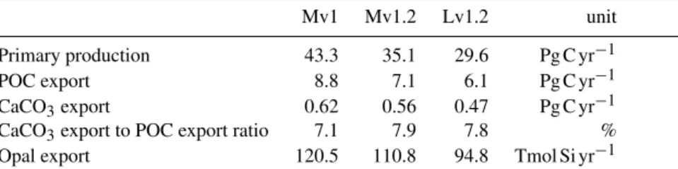
−0.004 Pg C yr⁻¹, with only small trends of 0.00007, 0.021, and−0.048 Pg C yr⁻¹century⁻¹for Mv1, Mv1.2, and Lv1.2, respectively. The relatively large uptake of carbon in Mv1 at the end of the spin-up is due to a lower CaCO₃ to POC production ratio found in this configuration. A full equilibra- tion of the model with respect to this process would require a considerably longer spin-up. The re-tuning of the ecosystem parameterisation, which increases CaCO₃production in version 1.2, leads to carbon fluxes much closer to zero at the end of the spin-up period. The larger trends in Mv1.2 and Lv1.2 compared to Mv1 despite longer spin-up time are due to larger decadal- to centennial-scale internal variability in these configurations (i.e. the systematic long-term drift is much smaller). We attribute this to the details of the salinity relaxation (balancing of the restoring flux, weaker relaxation south of 40^◦S). We finally note that even these larger trends are tiny compared to the changes in ocean carbon uptake due to anthropogenic carbon emissions, and that we calculate our estimates of anthropogenic carbon uptake relative to a con- trol run to account for offsets and trends due to a not fully equilibrated model.

Following the spin-up, we initialise two hindcast runs for each model version and configuration. The “historical” run uses prescribed atmospheric CO₂concentrations taken from the data set provided by Le Quéré et al. (2015). We start model integrations on 1 January 1762, since atmospheric CO2 begins to exceed the spin-up value of 278 ppm in this year. The second hindcast, which we call the “natural” run in this text, is continued with the constant pre-industrial CO2

concentration of 278 ppm. Northern and Southern Hemi- sphere tropospheric concentrations of CFC-11, CFC-12, and SF₆ are prescribed according to Bullister (2014). The historical and natural simulations continue to be forced by the CORE normal-year forcing until 1947. At 1 January 1948 we branch off historical and natural runs that are forced by CORE and NCEP-C interannually varying forcing (two historical and two natural runs for each model version and configuration). In the following sections we focus mainly on the

simulations forced with the NCEP-C-IAF data set, and all results presented have been obtained with this forcing unless explicitly stated otherwise.

2.5 Technical aspects

The HAMOCC code was originally written in FOR- TRAN 77. It was later re-written to take advantage of For- tran 90 elements (e.g. ALLOCATE statements) and to con- form to the Fortran 90 free source code format. Certain model options, such as the selection of a POC sinking scheme, are implemented via C-preprocessor directives. HAMOCC should compile on any platform that provides a FORTRAN compiler and a C-preprocessor.

MICOM is parallelised by dividing the global ocean do- main horizontally into (logically) rectangular tiles which are processed on one processor core each. Communication between cores is implemented using the Message Passing In- terface (MPI) standard. Since HAMOCC is integrated into MICOM as a subroutine call, it inherits this parallelism. Note that HAMOCC, in addition, has been parallelised for shared memory systems using the OpenMP standard. This feature is, however, not tested and not supported for the current set-up.

For the simulations presented in this paper, the ocean component has been run on 190 (Mv1), 309 (Mv1.2), and 155 (Lv1.2) cores on a Cray XE6-200 system, yielding a model throughput of 11 (Mv1), 20 (Mv1.2), and 64 (Lv1.2) simulated model years per (wall-clock) day.

3 Results and discussion 3.1 Physical model

3.1.1 Temperature and salinity

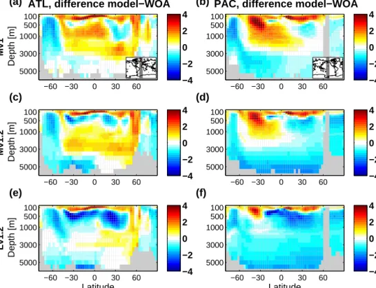
Zonal mean temperature (T) and salinity (S) differences between the model and the observation-based climatology from WOA 2009 (Locarnini et al., 2010; Antonov et al., 2010) for the Atlantic and Pacific basins are shown in Figs. 1 and 2. The general patterns ofT andSdeviations are similar across the different model versions and configurations. While all three configurations include salinity relaxation, this is not balanced in the case of Mv1, with the result that average salinity falls by 0.2 units during the course of the integration. The pre- dominantly negative salinity bias for the Mv1 configuration is visible in Fig. 2. The mid-latitude and tropical regions have a too strong temperature gradient in the upper 700 m, that is, a warm bias in the upper thermocline and a cold bias below.

While the magnitude and extent of the warm bias are similar for the three model configurations (up to≈4^◦C), the cold bias is weakest for Mv1, and strongest (up to−4^◦C) for low- resolution configuration Lv1.2.

In the Southern Ocean south of 50^◦S, the model is generally biased towards too cold and fresh conditions (about−1 to−2^◦C and up to−0.5 units on the Practical Salinity Scale)

(10)

Depth [m]

ATL, difference model−WOA (a)

Mv1

−60 −30 0 30 60 100

500 1000 3000 5000

−4

−2 0 2 4

Depth [m]

(c)

Mv1.2

−60 −30 0 30 60 100

500 1000 3000 5000

−4

−2 0 2 4

Latitude

Depth [m]

(e)

Lv1.2

−60 −30 0 30 60 100

500 1000 3000 5000

−4

−2 0 2 4

PAC, difference model−WOA (b)

−60 −30 0 30 60 100

500 1000 3000 5000

−4

−2 0 2 4

(d)

−60 −30 0 30 60 100

500 1000 3000 5000

−4

−2 0 2 4

Latitude (f)

−60 −30 0 30 60 100

500 1000 3000 5000

−4

−2 0 2 4

Figure 1.Temperature difference model−WOA averaged over 1965–2007 along zonal mean sections through the Atlantic/Southern Ocean (a, c, e)and the Pacific/Southern Ocean(b, d, f)for model configurations Mv1(a, b), Mv1.2(c, d), and Lv1.2(e, f). The regions covered by the zonal mean calculations are indicated by the grey shaded area in the insets of panels(a)and(b).

Depth [m]

ATL, difference model−WOA (a)

Mv1

−60 −30 0 30 60 100

500 1000 3000

5000 −0.5

0 0.5

Depth [m]

(c)

Mv1.2

−60 −30 0 30 60 100

500 1000 3000

5000 −0.5

0 0.5

Latitude

Depth [m]

(e)

Lv1.2

−60 −30 0 30 60 100

500 1000 3000

5000 −0.5

0 0.5

PAC, difference model−WOA (b)

−60 −30 0 30 60 100

500 1000 3000

5000 −0.5

0 0.5

(d)

−60 −30 0 30 60 100

500 1000 3000

5000 −0.5

0 0.5

Latitude (f)

−60 −30 0 30 60 100

500 1000 3000

5000 −0.5

0 0.5

Figure 2.As Fig. 1 but for salinity.

(11)

1800 1850 1900 12

14 16 18 20 22 24 26 28 30 32

Sv

Mv1 Mv1.2 Lv1.2

1948 1960 1980 2000

AMOC strength

year

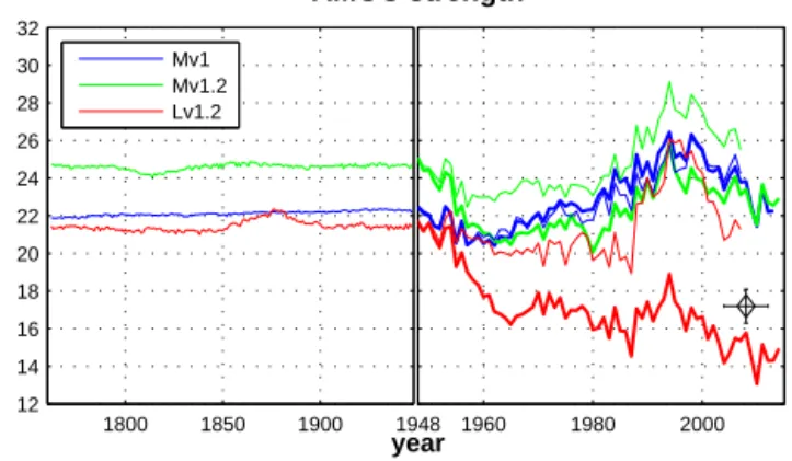
Figure 3. Atlantic Meridional Overturning Circulation (AMOC) measured as the maximum of the meridional stream-function at 26.5^◦N for Mv1 (blue lines), Mv1.2 (green), and Lv1.2 (red). The left panel shows the AMOC for the period 1762–1947 during which the model is forced with the CORE normal-year forcing. In the right panel the years 1948–2014 are shown, and thick (thin) lines indicate the overturning simulated with the model forced by the NCEP- C-IAF (CORE-IAF) data set. The black diamond with error bars indicates the observational estimate provided by McCarthy et al.

(2015).

below a slightly too warm surface layer. The layer of up- welled Atlantic deep water, which is warmer and more saline than Southern Ocean surface waters, is not or only weakly preserved in the model. At depths below 3000–4000 m the cold and fresh bias extends northwards into the Atlantic basin up to the Equator (a weak cold bias extends into the North Atlantic at depth). Above these bottom water masses and below the thermocline the Atlantic is generally too warm by 1 to 2^◦C and too saline by 0.2 to 0.5 units (again, salinity is biased low in Mv1 due to the unbalanced salinity restoring flux). In contrast, a warm and saline bias at intermedi- ate depths in the Pacific is mostly confined to the Southern Hemisphere, whereas the North Pacific is biased cold and fresh at all depths below 1000 m for all model configurations.

We note that the cold and fresh bias in the Southern Ocean water column is specific to the stand-alone configuration of the model and is not found in the fully coupled version of NorESM (e.g. Bentsen et al., 2013, Fig. 14).

3.1.2 Atlantic Meridional Overturning Circulation The Atlantic Meridional Overturning Circulation (AMOC) for the ocean-ice-only configuration of Mv1.2 has been compared to results from other models in Danabasoglu et al.

(2014). The forcing protocol for this latter study was to run the model through five cycles (1948–2007) of the CORE- IAF. The AMOC strength in our model, measured as the maximum of the annual mean meridional streamfunction at 26.5^◦N, varied between 12.5 and 19 Sv and showed an increasing trend of roughly 1 Sv century⁻¹. Under the spin-up with the CORE-NY forcing performed in the present work,

the AMOC shows a long transient increase in strength for about 300 years before stabilising. The average overturning for the 30 years before switching to interannual forcing (1918–1947) is 22.3, 24.8, and 21.5 Sv for Mv1, Mv1.2, and Lv1.2, respectively (Fig. 3, left panel). Aside from the abso- lute values we find similar curves of AMOC strength under the forcing protocol applied here (Fig. 3, right panel) compared to the results presented in Danabasoglu et al. (2014):

first a 10- to 15-year decrease by 2 to 4 Sv followed by a relatively stable phase until the early 1980s, an increase by 4 to 7 Sv towards a maximum in the late 1990s, and another decrease until the end of the simulation period (2007 or 2014).

The Lv1.2 configuration forced by NCEP-C-IAF is an out- lier in our small model ensemble. Compared to the other model simulations, the annual- and decadal-scale variability of AMOC strength appears to be similar but superimposed onto a negative trend of 8 Sv over the simulation period (see below).

In model configuration Mv1 we find only minor differences in AMOC strength between the simulation forced with CORE-IAF and the one forced with NCEP-C-IAF. For Mv1.2 and Lv1.2, however, the CORE-IAF simulations show a weaker initial decrease and a generally larger overturning than the corresponding NCEP-C-IAF simulations. These differences can be traced back to a peculiarity of the salinity relaxation scheme when the balancing of the relaxation flux is activated (not available in model version 1). Since too much salt is taken out of the surface ocean globally by the unbalanced scheme, negative salt fluxes are reduced by a multiplicative factor when balancing of the salinity relaxation flux is activated. Interestingly, the global restoring salt flux imbalance is larger when the model is forced with CORE-IAF. As a consequence of correcting this imbalance, we find a stronger reduction of the restoring salt flux out of the surface ocean in the simulations performed with CORE- IAF compared to those forced with NCEP-C-IAF. In the At- lantic north of 40^◦N, a positive salinity bias is therefore reinforced in the CORE-IAF simulations with model version 1.2, driving an increase in the AMOC relative to the simulations forced with NCEP-C-IAF. This effect is particularly pronounced in the Lv1.2 configuration, leading to the negative AMOC trend of 8 Sv described above. We note that the AMOC strength has been estimated as 17.2 Sv for the time period from April 2004 to October 2012 based on observations from the Rapid Climate Change programme (RAPID) array (McCarthy et al., 2015, diamond in Fig. 3). Compared to this value, our model overestimates the AMOC strength by about 4 to 9 Sv, except for the special case of Lv1.2 forced with NCEP-C-IAF discussed above, where AMOC is lower than the observational estimate by about 2 Sv for the period from 2004 to 2012.