Carbon Cycle
Fortunat Joos, Renato Spahni Physics Institute
University of Bern 2015
Table of Contents
1 INTRODUCTION ...7
1.1 The anthropogenic disturbance of the climate system ...7
1.1.1 The observed increase of greenhouse gases ... 7
1.1.2 Effect of the increase in greenhouse gas concentrations on the radiation balance ... 8
1.1.3 Impact of the greenhouse gas increase on the surface temperature ... 13
1.1.4 What to expect in the future?... 14
1.2 Variability of the atmospheric CO2 concentration in the past ...19
1.3 Rates of change and Radiative Forcing during the past 20’000 years ...24
2 THE MODERN CARBON CYCLE ... 29
2.1 Distribution of carbon in different reservoirs ...29
2.2 The anthropogenic CO2 perturbation ...32
3 THE TERRESTRIAL BIOSPHERE ... 39
3.1 Vegetation zones ...41
3.2 Fluxes and Inventories of carbon in the land biosphere ...46
3.2.1 A simple model for the description of the carbon content in vegetation and soil ... 50
3.3 Biospheric processes ... 53
3.3.1 Photosynthesis ... 53
3.3.2 Respiration ... 53
3.3.3 Regulation of photosynthesis and autotrophic respiration on the plant/leaf level ... 54
3.3.4 Regulation of the heterotrophic respiration ... 55
3.3.5 Seasonal changes of NPP, heterotrophic respiration and atmospheric CO2... 58
3.3.6 An estimate of potential changes in terrestrial carbon storage for a doubling of atmospheric CO2 ... 59
3.3.7 A concept model for the terrestrial sink flux ... 61
3.4 Photosynthesis-Transpiration ...66
3.4.1 Simplified description of photosynthesis in C3 plants ... 67
3.4.1.1 Limiting the rate of assimilation ... 68
3.4.1.2 Summary... 72
3.4.1.3 Temperature dependence of the model parameters... 72
3.4.1.4 Long-term effect of environmental conditions on photosynthesis ... 74
3.4.1.5 Production on the plant level ... 74
3.4.2 Evaporation and CO2 assimilation ... 75
3.4.2.1 Transpiration efficiency, W, on the plant level ... 76
3.4.3 Coupling of photosynthesis, evapotranspiration and soil water content ... 76
3.4.3.1 General concepts: ... 76
3.4.3.2 A model ... 76
3.4.4 Synopsis ... 78
3.5 Evaluation of terrestrial models ...79
3.6 Land Use Activities ...85
4 TRACER TRANSPORT IN THE OCEAN ... 93
4.1 Transient tracers: How fast does the atmospheric disturbance penetrate the ocean? ... 94
4.1.1 The 14C signal of above-ground nuclear bomb tests ... 94
4.1.2 Penetration of Chlorofluorocarbons into the ocean ... 95
4.1.3 The oceanic increase in DIC during the past 200 years: regional distribution ... 97
4.2 Stable tracers and the distribution of water masses ... 98
4.3 The radioactive carbon isotope 14C: How quickly does the Ocean mix? ... 100
5 UPTAKE OF ANTHROPOGENIC CO2 BY THE OCEAN ... 103
5.1 Processes and models ... 103
5.1.1 CO2-exchange flux atmosphere-ocean ... 104
5.1.2 Carbonate chemistry ... 112
5.1.3 Long-term CO2 uptake by the ocean ... 120
5.1.4 Uptake of anthropogenic CO2: A simple model ... 120
6 THE MARINE BIOLOGICAL CYCLE ... 125
6.1 A geochemical perspective ... 125
6.2 Biological processes in the euphotic zone and re-mineralization of organic matter at depth ... 135
6.2.1 Limiting factors for biological production ... 139
6.2.2 Export Production ... 142
6.2.3 Re-mineralization of organic matter at depth ... 143
6.2.4 Apparent Oxygen Utilization ... 144
6.2.5 Nitrous Oxide (N2O) ... 148
6.2.6 Calcium carbonate ... 151
6.3 Glacial-interglacial CO2 variations ... 164
B. Stocker is acknowledged for the translation of the German version of this manuscript and A. Bozbiyik for help with the formatting.
1 Introduction
The global cycles of carbon (C), oxygen (O) and of various other elements (N, P, Si, Fe, etc.) form a global biogeochemical cycle. This means that biological, geological, chemical and physical processes play a role. The cycles of the different elements are linked to each other, e.g. C, H2O and O. For several reasons, the carbon cycle plays a key role in the Earth system:
It affects the buildup and turnover rates of the entire biosphere. Carbon cycle, water cycle, oxygen cycle and the energy budget are coupled by the exchange of CO2, O2 and water with the biosphere.
It affects the global radiation balance. Two most important greenhouse gases, but ranking after water vapor in importance, are carbon dioxide (CO2) and methane (CH4). Both contain carbon and their atmospheric concentration has been growing at an increasing rate since the industrial revolution (starting at around 1800 AD).
A change of the radiation balance may cause irreversible changes in the climate system.
Out of 1,000 g carbon, added to the atmosphere by burning fossil fuels, over 70 g remain in the atmosphere for several millennia (1st order irreversibility). In the non-linear climate system, an altered temperature regime can lead to a shift of its equilibrium (2nd order irreversibility) and hence to considerably different distributions of temperature, precipitation, etc.
It affects the distribution of nutrients and oxygen in the ocean. The distribution of tracers, the ocean circulation and the carbon cycle are tightly coupled.
Past variations of the atmospheric CO2 and CH4 concentrations and of the oceanic distribution of nutrients and carbon isotopes are recorded in Antarctic ice and ocean sediments. Measuring these variables in ice cores and oceanic sediment cores reveals quantitative information about past states of the climate system.
This lecture is concerned with two key questions:
1. How will the atmospheric CO2 concentration, the climate and the interaction between climate and CO2 evolve in the future?
2. How can we explain past variations in atmospheric CO2 and climate?
1.1 The anthropogenic disturbance of the climate system
1.1.1 The observed increase of greenhouse gases
Throughout the past 200 years and particularly since World War II, human activities have caused an enormous disturbance of global biogeochemical cycles and climate. The increase in atmospheric CO2and other greenhouse gases is well documented thanks to a combination of atmospheric and ice core data. Over the course of the last millennium and before the industry- alization, the atmospheric concentrations of CO2, CH4 und N2O were roughly constant.
Today, concentrations of these greenhouse gases are higher than during the past 800’000 years.
The atmospheric CO2 concentration is commonly expressed as a molar ratio in units of ppm (parts per million in dry air: 10-6). 1 ppm corresponds to an atmospheric inventory of 2.123 1012 kg C. The molar ratio of CH4 and N2O is given in ppb (parts per billion, 10-9).
Figure 1.1: The rise in greenhouse gases CO2, CH4, und N2O. In the past decades, the increase in the atmosphere has been directly measured with air samples, e.g., since 1958, regular measurements of CO2 have been conducted on Mauna Loa (Hawaii). For earlier periods, measurements of air extracted from Antarctic ice cores are available (The Physical Institute of the University of Bern is involved in such measurements).
1.1.2 Effect of the increase in greenhouse gas concentrations on the radiation balance
The rise in atmospheric greenhouse gas concentrations and aerosols is associated with a considerable disturbance of the radiation balance of the Earth-surface/troposphere system.
This disturbance of the radiation balance is referred to as Radiative Forcing. The Radiative Forcing of the surface-troposphere system by a perturbation, e.g., an increase in greenhouse gases, is equal to the change in net radiation (incident minus outgoing, short- and long-wave) that would pass the tropopause if the temperature and the state of the troposphere and the
Earth surface remained unchanged. The Radiative Forcing by well-mixed greenhouse gases is well known, whereas uncertainties in Radiative Forcing for other drivers are larger and particularly the effects of aerosols are relatively poorly understood.
As a first order approximation, the Radiative Forcing is a good indicator for the resulting change in the global mean temperature at the Earth surface. After attaining a new equilibrium, the change in the global mean temperature, Ts, and the Radiative Forcing, RF are linked by the climate sensitivity :
,
,
0 and thus
s
s
RF T RF
T
Eq. 1.1
A change in Radiative Forcing leads to an altered radiation balance and the corresponding radiative response is given by TS. The climate sensitivity is not accurately known due to numerous complex feedback mechanisms, e.g. an increase in RF leads to more water vapor in the atmosphere due to warming (positive feedback), changed cloud cover (positive as well as negative feedbacks) and a decrease of the snow- and ice cover (positive feedback).
Figure 1.2: Estimates for the global mean Radiative Forcing in 2011 relative to 1750 for different drivers. (IPCC WGI, 2013, Figure SPM.5)
Radiative transfer models that resolve the 3-dimensional structure of the atmosphere, as well as the absorption of individual bands, yield the following (parameterized) relationship between atmospheric CO2 and global Radiative Forcing:
( )
) ln (
m W 35 . 5 ) (
0 2
2 2
-
t CO
t t CO
RF Eq. 1.2
CO2(t0) represents the preindustrial reference concentration. For a doubling of the atmospheric CO2 concentration, the Radiative Forcing is equal to 3.7 W m-2 with an uncertainty of around 10%. Similar parameterizations exist for other anthropogenic greenhouse gases and aerosols. The CO2 forcing increases with the logarithm of its concentration, due to ‘self-shading’. Similarly, the Radiative Forcings of CH4 and N2O increases with the square root of their concentrations. Thus, an identical increase in concentration leads to a higher Radiative Forcing at low concentrations than at high concentrations. In contrast, for gases occurring at low concentrations (e.g. CFCs) the Radiative Forcing increases linearly with the atmospheric concentration.
agent equation Co
CO2 RF = 5.35 W m-2 ln(CO2/CO2,o) 278 ppm
CH4 RF = 0.036 W m-2 CH4 CH4,0
fCH4,,N2O0 f CH4,0,,N2O0 742 ppb N2O RF = 0.12 W m-2 N2O N2O0
fCH4,o,,N2O fCH4,0,,N2O0 272 ppb
CFC-11 RF = 0.25 W m-2 (CFC-11 – CFC-110) 0 ppt
CFC-12 RF = 0.32 W m-2 (CFC-12 – CFC-120) 0 ppt
Table 1.1: Equations for the calculation of the Radiative Forcing for different greenhouse gases, relative to a preindustrial (1750 A.D.) reference concentration (C0). The overlap of the absorption bands of N2O und CH4 is accounted for by the function f(M,N)=0.47 ln(1+2.01x10⁻⁵ (MN)0.75+5.31x10⁻¹⁵ M(MN)1.52). However, this term is small.
Often, the climate sensitivity is expressed as the increase of the equilibrium temperature, T (2xCO2), in response to a doubling of the atmospheric CO2 content. Once the climate system has attained a new equilibrium, the change in the global surface temperature is equal to
) 2
( 2
2
, RF xCO
T RF Ts x
Eq. 1.3
It follows:
2 2
(2 )
x
RF xCO
T
Eq. 1.4
The ‘warming commitment’ by today’s Radiative Forcing from well-mixed anthropogenic greenhouse gases can be derived by the equations above. For a mean climate sensitivity of 3oC and a current Radiative Forcing of about 2.5 W m-2, we expect an equilibrium warming of 2oC relative to the preindustrial global mean surface temperature. We note that a considerable part of the greenhouse forcing is compensated by the cooling effect of aerosols and the climate system is currently not in equilibrium. The warming lags the forcing due to the large thermal inertia of the ocean.
The geographical distribution of the Radiative Forcing is different for well-mixed atmospheric gases (CO2, CH4, N2O, CFCs) and for short-lived substances with regionally
variable concentrations (ozone, aerosols). For well-mixed gases, the disturbance of the radiation balance is largest in the subtropical zone and lowest at the poles, corresponding to the distribution of the long-wave outgoing radiation. The annual mean Radiative Forcing is slightly reduced at the Equator compared to the subtropics due to high cloud cover in the intertropical convergence zone.
Figure 1.3: Geographical distribution of the annual mean Radiative Forcing (1750 to 2000) by the well mixed greenhouse gases CO2, CH4, N2O, CFC-11 and CFC-12 in W m-2.
Box 1.1
By how much would global mean surface temperature rise for a doubling of atmospheric CO2?
a) Planetary radiation temperature. Let us consider the Earth as a black body with radius rp. According to the Stefan-Boltzmann law, the emitted radiation for a body with temperature T is:
4 Planck
h T black body radiation per unit area; sign indicates outgoing In equilibrium: absorbed incident radiation = emitted planetary radiation :
2 4 2
0 p p e,0 p
S r (1 ) T 4 r 0 , it follows:
4 0
e,0 p
T S (1 )
4
and further:
1 1 4 0
e,0 p
T S (1 )
4
For the Earth:
p 0.3
Planetary albedo: 30% of the incoming radiation is reflected.
S0 =1367 W m-2 Solar irradiance at the top of the atmosphere (TOA)
10 8 57 ,
5
W m-2 K-4 Stefan Boltzmann constant
Te,0 = 255 K planetary radiation temperature (calculated).
b) climate sensitivity , The equilibrium change in outgoing radiation in response to a Radiative Forcing, RF, balances RF and it holds at equilibrium: RF+h=0.
We linearize the response in h as a function of T:
e ,0 e ,0
* * 2
s, s,
T T T T
h h
h T + f(( T ) )+.. and define
T T
s, s,
It follows: RF+ T =0, and thus T RF
The climate sensitivity with regard to the black body radiation, Planck, is:
e ,0
Planck 3
Planck e,0
T T
h 4 T
T
and evaluation in 3-d yields: Planck= 3.1 (W m-2) K-1 c) Equilibrium change in surface temperature, TS, for a doubling of atmospheric CO2. The Radiative Forcing is calculated according to:
-2 2
0
CO2(t )
RF(CO ) 5.35 ln W m 5.35 ln 2
CO2(t )
W m-2= 3.7 W m-2
This yields when considering only the Planck feedback:
* -2 -2 1
s, Planck
T RF / (3.7 W m ) / (3.1 W m K 1.2 K
Feedback mechanisms: Other feedback mechanisms such as an increase in water vapor and a decrease in planetary albedo due to reduced ice and snow extent as well as changes in cloud properties affect the climate sensitivity. The confidence interval for the climate sensitivity is:
T2xCO2 = [1.5 - .4.5 K] equilibium surface temperature change for a doubling of CO2, or a Radiative Forcing of 3.7 W m-2.
1.1.3 Impact of the greenhouse gas increase on the surface temperature The largest portion of the observed warming of the last 50 years is probably due to the increase in greenhouse gases. The global mean temperature at the Earth surface has been increasing ever since instrumental records are available. The global temperature increase of the 20th century is 0.60.2 oC. The warming was strongest in continental regions of the northern hemisphere, while the ocean and the southern hemisphere have witnessed a smaller warming. The observed mean northern hemispheric temperatures of the past years appear to lie outside the range of variability of the past millennium. Preindustrial temperature changes are reconstructed based on proxy data (tree rings, ice cores, sediments).
Figure 1.4: Increase of the global mean temperature (above) and the mean temperature of the northern hemisphere (below). Sufficient instrumental data for a reconstruction of the mean global temperature exists since 1860. The temperature before 1860 is reconstructed based on proxy data, predominantly tree ring analyses.
These reconstructions are subject to different uncertainties and in some cases the different reconstructions disagree strongly.
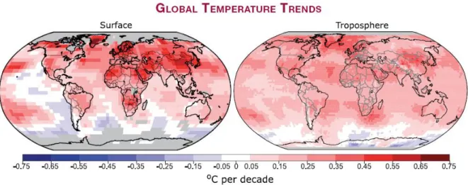
Figure 1.5: Patterns of estimated linear global temperature trends over the period 1979 to 2005 for the surface (left), and for the mid-troposphere from satellite records (right). Grey indicates areas with incomplete data. Rates of increase are generally larger over land than over ocean. (IPCC, 2007)
1.1.4 What to expect in the future?
Figure 1.6: Radiative forcing and projected change in global means surface temperature (relative to 1986-2005) for the Representative Concentration Pathways (RCP) used by the Intergovernmental Panel on Climate Change (WGI, 2013, Figure TS.15). Solid lines are multi-model mean and the shading indicates the 5-95% interval across the distribution of models. RCP8.5 and RCP6 are pathways assuming no climate-policy intervention.
Radiative forcing is assumed to stabilize after 2100 in all scenarios.
Figure 1.7: Compatible fossil-fuel emissions simulated by the CMIP5 models for the four Representative Concentration Pathways. The inset shows prescribed CO2 concentrations. Solid lines are multi-model means; shading denotes the ±1 standard deviation range of individual model annual averages.
(IPCC WGI, 2013, Figure TS.19)
Business as Usual: Without any climate-policy measures, greenhouse gas concentrations in the atmosphere will continue to increase and the rate of climate change is going to increase compared to the 20th century. Non-intervention scenarios for different possible development pathways of population, economy and technology point to sustained high CO2 emissions. The emissions cause a further CO2 increase in the atmosphere, an increase of global surface temperature, sea level rise, altered precipitation patterns, an increase in ocean acidity and a reduction in Arctic sea ice extent.
The modeled temperature and precipitation responses to the scenarios of the Inter- governmental Panel on Climate Change differ significantly depending on the season and region. The modeled temperature increase is the largest in continental regions and stronger in the northern than in the southern hemisphere. This is consistent with the observed trends of the past decades. While most models reveal a consistent picture of the temperature increase, results regarding to the projected precipitation changes show a stronger disagreement.
However, an increase in the amount of precipitation is very likely in high latitudes, while a decrease is likely in most subtropical continental regions.
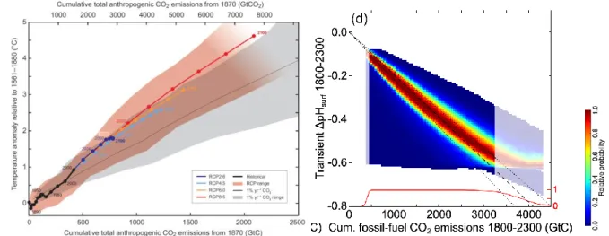
Many changes increase (approximately linearly) with cumulative carbon emissions:
Figure 1.8: Relationship between cumulative carbon emissions and changes in global mean (left) surface air temperature and (right) surface ocean pH (IPCC WGI, 2013, Figure SPM.10 and Steinacher and Joos, BGD, 2015).
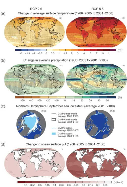
Figure 1.9: Maps of CMIP5 multi-model mean results for the scenarios RCP2.6 and RCP8.5 in 2081–2100 of (a) annual mean surface temperature change, (b) average percent change in annual mean precipitation, (c) Northern Hemisphere September sea ice extent, and (d) change in ocean surface pH. Changes in panels (a), (b) and (d) are shown relative to 1986–2005. For panels (a) and (b), hatching indicates regions where the multi- model mean is small compared to natural internal variability (i.e., less than one standard deviation of natural internal variability in 20-year means). Stippling indicates regions where the multi-model mean is large compared to natural internal variability (i.e., greater than two standard deviations of natural internal variability in 20-year means) and where at least 90% of models agree on the sign of change. In panel (c), the lines are the modelled means for 1986−2005; the filled areas are for the end of the century. The CMIP5 multi-model mean is given in white colour, the projected mean sea ice extent of a subset of models (number of models given in brackets) that most closely reproduce the climatological mean state and 1979 to 2012 trend of the Arctic sea ice extent is given in light blue colour. (IPCC WG, 2013, Figure SPM.8).
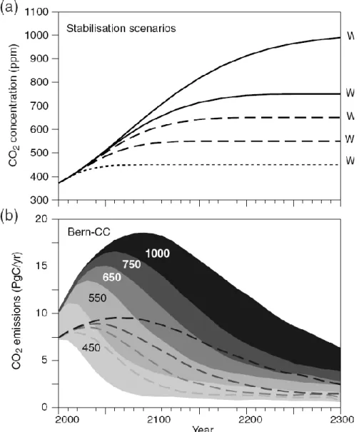
Stabilization of the greenhouse gas concentrations: Article 2 of the United Nations Framework Convention on Climate Change (UNFCC, Rio 1992) requires a stabilization of greenhouse gases in the atmosphere in order to prevent a dangerous anthropogenic disturbance of the climate system. CO2 emitted by the combustion of fossil fuels accumulates in the climate system. A stabilization of CO2 concentration in the atmosphereand thereby a slowdown and a long-term stabilization of anthropogenic temperature and climate changes requires a trend reversal with respect to the emissions and a reduction of carbon emissions below today’s rate.
Anthropogenic warming and sea level rise would continue for centuries due to the time scales associated with climate processes and feedbacks, even if greenhouse gas concentrations were to be stabilized.
Figure 1.10: Projected CO2 emissions leading to a stabilization at different CO2 concentrations. Stabilization pathways (upper panel) were prescribed in a carbon cycle model (lower panel). The ranges represent the uncertainties resulting from different extreme model assumptions. For all stabilization scenarios, carbon emissions need to be reduced below today’s level (From IPCC Third Assessment Report, Technical Summary, WGI).
Box 1.2
What fraction of fossil fuel resources could be combusted over the next 1000 years if atmospheric CO2 were to be stabilized at twice the preindustrial concentration?
Conservative estimates of the fossil fuel reserves amount to some 5000 GtC (without accounting for the huge reserves of methane clathrates). On a time scale of several hundred years, ocean and atmosphere carbon inventories equilibrate and after 1000 years, about 20 % of the fossil emissions remain in the atmosphere (the possible C-uptake of the biosphere is small compared to the long-term ocean uptake). This results in a fraction r of the fossil fuel reserves that could be combusted, in order to stabilize CO2 at around 560 ppm:
-1 2,0
1 1
(560 ppm CO ) 280 ppm 2.123 GtC ppm
Emission 0.2
r 0.6
Resources Resources 5000 GtC
CO2,0 280 ppm preindustrial CO2 concentration
2.123 GtC ppm-1 conversion factor (1 ppm in the entire atmosphere is equivalent to an atmospheric inventory of 2.123 GtC.)
~0.2 airborne fraction (fraction of the emissions that remains in the atmosphere)
Abrupt and irreversible climate change: The possibility of abrupt and irreversible changes in the climate system is real. From palaeodata, we know that a complete shut-down of the deep water formation in the North Atlantic is possible (Figure 1.11).
Figure 1.11: Multi-model projections of Atlantic Meridional Overturning Circulation (AMOC) strength at 30°N from 1850 through to the end of the RCP8.5 extension (IPCC WGI, 2013, Figure 12.35).
Models show a reduction of the deep water formation during the 21st century in the North Atlantic, which results in a decreased meridional heat transport. For constantly high greenhouse gas concentrations, some models simulate a complete and irreversible collapse of the North-Atlantic circulation.
1.2 Variability of the atmospheric CO2 concentration in the past
Measurements of the CO2 concentration provide valuable information about the climate in the past. To understand past changes in the climate system consistently, qualitatively and quantitatively remains a major challenge in climate physics. CO2 concentrations and climate have been varying on all time scales throughout the Earth’s history.
Figure 1.12: Variations of the atmospheric CO2 concentration on different time scales.
Geological time scale: The CO2 concentration was very high (> 3‘000 ppm) between 600 and 400 million years before present (BP) and between 200 and 150 million years BP. On very long time scales, the atmospheric concentration is governed by the balance between geochemical source and sink processes, such as sedimentation of organic carbon in the ocean, erosion and volcanism. The formation of the terrestrial biosphere increased the erosion rate of silicate rocks which is a sink of CO2. The net effect of this slight disequilibrium in the carbon cycle that was maintained over hundreds of millions of years was a reduction of the atmospheric CO2 concentration. In the geologically younger past, the CO2 concentration decreased further and there is evidence that the concentrations during the last 20 million years did not exceed 300 ppm.
Glacial-interglacial: Past atmospheric CO2 concentrations can be reconstructed from measurements on air trapped in Arctic and Antarctic ice cores. The atmospheric CO2
concentration varied between 180 and 300 ppm. The lowest concentrations are associated with periods of maximum glaciation and the highest values to warm periods. Variations of the Earth’s orbital parameters (Milankovic Theory) are assumed to be the ultimate driver of the Glacial-Interglacial cycles. CO2 is one of the different parameters of the Earth system that exhibits the typical Milankovic frequencies of the orbital parameters. The variation in the greenhouse gas concentrations amplified the glacial-interglacial climate change.
Figure 1.13: Variations of the greenhouse gases N2O, CO2 and CH4, Deuterium in ice (a proxy for temperature) and 18O in shells of bottom-dwelling organisms preserved in marine sediments (a proxy for ice volume/sea level) over the past 800’000 years. The data was retrieved from ice cores of Vostok, Antarctica and Dome Concordia (Antarctica) and from a stack of marine sediments (Lisiecki and Raymo, 2005). For a comparison, the greenhouse gas records were extended with data of the anthropogenic increase of the past 200 years (stars). The last five interglacials are highlighted with grey bands. The CO2 and deuterium records correlate strongly. The somewhat colder warm phases between 450’000 and 800’000 years BP are associated with lower CO2
concentrations than during the more recent, warmer interglacials.
Variations during the glacial period: Detailed measurements show that the CO2
concentration also varied on shorter time scales. Variations in the CO2 concentrations of up to 20 ppm are found. These are related to warm period in the Antarctica and the so-called Dansgaard-Oeschger warm-cold oscillations. These climate shifts are linked to changes in the ocean circulation and the heat transport in the North Atlantic, which lead to opposite temperature changes in the two hemispheres.
Figure 1.14: Variations of the temperature indicator 18O in Greenland ice (Greenland Ice Core Project, GRIP), the temperature as derived form 18O measurements on an Antarctic Ice core (Vostok) and the CO2 content in the atmosphere. Arrows (H2 and H6) represent Heinrich Events (input of ice/freshwater into the North Atlantic) and the numbers represent (relative) warm phases in Greenland (Interstadials 2-18) and in Antarctica (A1-A4).
The catastrophic discharge of large ice masses (freshwater of low density) into the North Atlantic, recorded by the so-called Heinrich-layers in oceanic sediments, probably led to a temporary collapse of the deep water formation in the North Atlantic and to a reduction in the pole-ward heat transport. Increased CO2 concentrations are found during the warm phases in Antarctica. Also during the last glacial-interglacial transition, different trends in CO2 are detected. The CO2 variations during the last glacial period are relatively small and demonstrate that under natural conditions, the CO2 concentration is well buffered against abrupt climate change, in particular against a shut-down of the North Atlantic deep water formation.
Event, Stadial Estimated age in 1000 years before present (kyr BP)
Holocene (current interglacial period) 10 kyr BP until today Transition glacial-Holocene 18 to 10 kyr BP
Termination 1 14 kyr BP
Younger Dryas (YD) 12.7 to 11.5 kyr BP
Antarctic cold reversal 14 to 13 kyr BP Bölling-Alleröd warm period 14.5 to 13 kyr BP
Last Glacial 74 to 14 kyr BP
Last Glacial Maximum (LGM) 25 to 18 kyr BP Eemian/Marine Isotope Stadial 5e 128 to 118 kyr BP Peak of the last Interglacial 124 kyr BP
Termination 2 130 kyr BP
Heinrich event Large amounts of ‘ice rafted debris’ in marine sediments, reoccurrence after 7-10 kyr
Dansgaard-Oeschger cycles Warm-cold oscillations during the last glacial, period with a duration of a few kyrs, detected in Greenland ice cores
Termination Period of fast ice retreat
Table 1.2: Terminology used in paleoclimatic studies covering the past 150’000 years.
Variations during the Holocene: Measurements on ice of Taylor Dome and Dome C in Antarctica show that the CO2 concentration at the beginning of the present warm period decreased slightly and increased again between 7 kyr BP and preindustrial by about 20 ppm.
Measurements of the stable isotope 13C constrain possible mechanisms responsible for this increase. The CO2 concentration varied by a few ppm during the last millennium before the anthropogenic increase. The low natural variability of CO2 and other greenhouse gases during the last millennium points to relatively small global climate variations.
Figure 1.15: Variations of the atmospheric CO2 concentration and of the 13C:12C isotope ratio during the Holocene (Note reversed age scale). The isotope ratio permits the quantification of different carbon source and sinks with different isotopic signatures.
Interannual and seasonal variations: Today, CO2 measurements on atmospheric air are conducted routinely at around 40 stations worldwide. Considerable variability in the annual rate of atmospheric CO2 increase is detected. The seasonal variation has an amplitude of a few ppm. The seasonal signal is mainly caused by the exchange with the land biosphere and decreases from north to south. This gradient is linked to the larger land fraction in the northern compared to the southern hemisphere.
Figure 1.16: CO2 concentration in air as recorded at stations located in different latitudes. The amplitude of the seasonal variability decreases from south to north.
1.3 Rates of change and Radiative Forcing during the past 20’000 years
Figure 1.17: Changes in the atmospheric concentration of CO2, CH4, N2O and rates of change of their combined Radiative Forcing during the past 20’000 years. Records from different ice cores from Antarctica and Greenland (symbols) are extended with direct atmospheric measurements. Radiative Forcing relative to 1750 is given on a non-linear scale on the right side. The grey bars represent measured values for the past 650’000 years. Variations in the atmospheric CO2 dominate the Radiative Forcing of all three gases combined. The mean decadal rate of increase in Radiative Forcing (lower right) is six times larger than at any time during the past 20’000 years. Air trapped in ice reveals a smoothing of the atmospheric signal. The range of the age distribution of the air trapped in ice varies between 20 years in regions with a high accumulation of snow and 200 years for regions with low accumulation rates. The rates determined from the high-resolution Law Dome ice and firn records of the past 2000 years are given by the thin black line in the lower right figure. The arrow shows how the anthropogenic peak would be damped in places with low accumulation.
Figure 1.18: Rates of change for the three greenhouse gases, N2O, CH4, CO2 and their combined radiative forcing for the last 22 ka. The Greenland CH4 data represent decadal-scale variations and inferred rates of change (dash) are directly comparable for different periods. The black lines/arrows show the peak in the rate of change in radiative forcing and concentrations after the anthropogenic signals of CO2, CH4 (no arrow shown), and N2O have been smoothed with a model describing the enclosure process of air in ice.
The rate of increase in concentrations and in Radiative Forcing of the three greenhouse gases CO2, CH4, N2O is accelerating. Radiative Forcing of CO2 varied by less than 0.1 milliwatt m-2 yr-1 during the past 6000 years before the Industrialization, but already by about 12 milliwatt m-2 yr-1 during the 20th century and by about 27 milliwatt m-2 yr-1 during the past decade (1994 to 2003).
Figure 1.19: Radiative perturbations for the Last Glacial Maximum (21’000 years BP) relative to 1750 A.D. for different forcings/feedbacks (from Jansen et al., 2007).
Figure 1.2 and Figure 1.19 allow us to compare the well-known forcings of the radiation balance for today and the period of the LGM. The glacial-interglacial cycles were most likely driven by the changes of the Earth’s orbit around the sun. However, the change in global mean radiation is too small to explain the reconstructed temperature change between today and the LGM. Other mechanisms amplified the orbital forcing. The increase in albedo due to the extent of ice sheets is the largest individual forcing at the LGM. The drivers linked to the biogeochemical system (greenhouse gases, dust, vegetation cover) are responsible for more than half of the LGM-forcing. This highlights the central role of biogeochemical cycles in the climate system.
The changes of the Earth orbit cause relatively small changes in the total solar energy input.
However, at the LGM, the energy was distributed differently between seasons and latitude.
The Radiative Forcing today is the result of the partly cancelling contributions from well- mixed greenhouse gases (CO2, CH4, N2O and CFCs), stratospheric and tropospheric ozone, different aerosols and changes in land use and solar energy output. In the near future, the CO2 forcing will gain importance since emitted CO2 is accumulating in the atmosphere, sulphur emissions are decreasing and methane concentrations are not increasing at this point of time.
From Sections 1.1, 1.2 and 1.3 the following conclusions emerge:
1. The 20th century increase in CO2 and its radiative forcing occurred more than an order of magnitude faster than any sustained change during the past 22,000 years.
2. Today’s atmospheric CO2 concentration is higher than ever during the past 800’000 years and probably the past 20 million years.
3. Greenhouse gases and the biogeochemical system play a central role for past and future climate change.
Literature:
Excellent book on the ocean carbon cycle:
Sarmiento, J. & Gruber, N. (2006) Ocean Biogeochemical Dynamics (Princeton University Press).
Reviews:
T. F. Stocker et al., in Climate Change 2013: The Physical Science Basis. Contribution of Working Group I to the Fifth Assessment Report of the Intergovernmental Panel on Climate Change, T. F. Stocker et al., Eds.
(Cambridge University Press, Cambridge, United Kingdom and New York, NY, USA, 2013), pp. 33-115.
http://www.ipcc.ch/report/ar5/wg1/
Solomon, S., Qin, D., Manning, M., Alley, R., Berntsen, T., Bindoff, N. L., Chen, Z., Chidthaisong, A., Gregory, J., Hegerl, G., Heimann, M., Hewitson, B., Hoskins, B., Joos, F., Jouzel, J., Kattsov, V., Lohmann, U., Matsuno, T., Molina, M., Nicholls, N., Overpeck, J., Raga, G., Ramaswamy, V., Ren, J., Rusticucci, M., Somerville, R., Stocker, T. F., Stouffer, R. J., Whetton, P., Wood, R. A. & Wratt, D. (2007) in Climate Change 2007: The Physical Science Basis. Contribution of Working Group I to the Fourth Assessment Report of the Intergovernmental Panel on Climate Change, eds. Solomon, S., Qin, D., Manning, M., Chen, Z., Marquis, M., Averyt, K. B., Tignor, M. & Miller, H. L. (Cambridge University Press, Cambridge United Kingdom and New York, NY, USA), pp. 19-91.http://www.ipcc.ch
Prentice, I. C., G. D. Farquhar, M. J. Fasham, M. I. Goulden, M. Heimann, V. J. Jaramillo, H. S. Kheshgi, C.
LeQuéré, R. J. Scholes, and D. W. R. Wallace. 2001. The carbon cycle and atmospheric CO2. Pp. 183–237 in Climate change 2001: The scientific basis (Contribution of Working Group I to the third assessment report of the Intergovernmental Panel on Climate Change), edited by J. T. Houghton, Y. Ding, D. Griggs, M. Noguer, P. van der Linden, X. Dai, K. Maskell, and C. A. Johnson. Cambridge: Cambridge University Press. http://www.proclim.ch/IPCC2001.html; http://www.ipcc.ch
Joos F. and I. C. Prentice. A paleo-perspective on changes in atmospheric CO2 and climate. In Towards Stabilization of Atmospheric CO2, C. Field and M. Raupach (Eds.), SCOPE/GCP rapid assessment of the carbon cycle, Island Press, in press, 2004. http://www.climate.unibe.ch/~joos/publications.html
Stocker, T. F. 2000. Past and future reorganisations in the climate system. Quaternary Science Reviews 19:301–
319. http://www.climate.unibe.ch/publications.html
Others (results from ice cores)
Elsig, J., Schmitt, J., Leuenberger, D., Schneider, R., Eyer, M., Leuenberger, M., Joos, F., Fischer, H. and Stocker, T. F.: 2009, Stable isotope constraints on Holocene carbon cycle changes from an Antarctic ice core, Nature 461: 507–510. http://www.climate.unibe.ch/~joos/publications.html
Petit, J. R., J. Jouzel, D. Raynaud, N. I. Barkov, J.-M. Barnola, I. Basile, M. Bender, J. Chappellaz, M. Davis, G.
Delayque, M. Delmotte, V.M. Kotlyakov, M. Legrand, V.Y. Lipenkov, C. Lorius, L. Pépin, C. Ritz, E.
Saltzman, and M. Stievenard. 1999. Climate and atmospheric history of the past 420,000 years from the Vostok ice core, Antarctica. Nature 399:429–436.
Lüthi, D., et al. (2008), High-resolution carbon dioxide concentration record 650'000-800'000 years before present, Science, 453, 379-382
Monnin, E., A. Indermühle, A. Däallenbach, J. Flückiger, B. Stauffer, T. F. Stocker, D. Raynaud, and J. Barnola.
2001. Atmospheric CO2 concentrations over the last glacial termination. Science 291:112–114.
http://www.climate.unibe.ch/publications.html
Siegenthaler, U., Stocker, T. F., Monnin, E., Luthi, D., Schwander, J., Stauffer, B., Raynaud, D., Barnola, J. M., Fischer, H., Masson-Delmotte, V. & Jouzel, J. (2005) Science 310, 1313-1317.
2 The modern carbon cycle
2.1 Distribution of carbon in different reservoirs
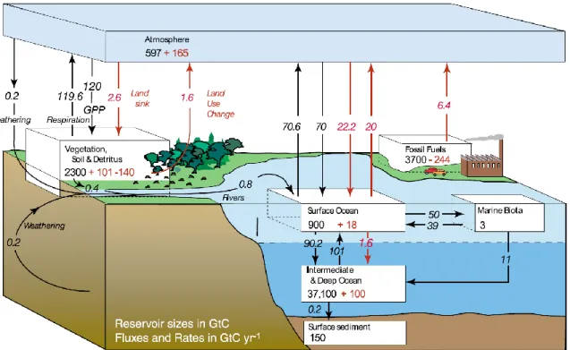
Quantities and exchange fluxes of the most important carbon reservoirs are summarized in Figure 2.1 and Table 2.1. The carbon cycle is considerably disturbed by the carbon release from fossil fuel burning and deforestation and other land use activities. The reservoirs atmosphere, biosphere, ocean and sediments are characterized as follows:
Atmosphere: Carbon in the atmosphere is most commonly present in the form of carbon dioxide (CO2; 2000: 368 ppmv), methane (CH4, 2000: 1.7 ppmv = 1700 ppbv; parts per billion by volume) and carbon monoxide (CO; 50...100 ppbv). The atmospheric CO2 concentration affects the radiation balance and thus physical climate. The CH4 concentration has more than doubled during the past 200 years. The greenhouse effect of a single CH4 molecule is much higher than that of a CO2 molecule. However, its atmospheric concentration is two orders of magnitude smaller than CO2.
Box 2.1
Biosphere: A highly simplified formula for organic material is CH2O, or C6H12O6 (glucose).
The fluxes passing the terrestrial and marine biosphere are of similar magnitude, but the mean residence times differ markedly due to different reservoir sizes (see Table 2.1): they are ~10 years for the living terrestrial biosphere (without soils) and 1 month for the marine biosphere.
Box 2.2
Ocean: With its 40’000 GtC, the ocean is the largest rapidly exchanging carbon reservoir (‘rapid’ in this context means < 1000 years). Carbon is most abundant in the form of dissolved inorganic carbon. The denomination CO2 or DIC refers to the sum of bicarbonate (HCO3; about 90%), carbonate (CO32; about 10%) and dissolved gaseous CO2 (about 0.5%). A small amount of the total carbon in the ocean (a few percent) is in the form of dissolved organic carbon, DOC.
Residence time: A useful first order measure to characterize the time scale of exchange processes is the residence time of carbon in a reservoir. The mean residence time, , of a substance in a reservoir of mass M and discharge F is:
F
M
Units: Global amounts of carbon are commonly quantified in GtC (gigatons of carbon 1 GtC = 109 tC = 1015 g C) or in mol (1 mol-C=12.01 gram). Independent from its chemical form, only the amount of C-atoms are quantified. The atmospheric CO2 concentration is usually given as a mixing ratio in ppm (parts per million (volume)= 1 CO2 molecule per 106 molecules of dry air). A mean mixing ratio of 1 ppm corresponds to an atmospheric inventory of 2.123 GtC.
Figure 2.1: The global carbon cycle for the 1990s, showing the main annual fluxes in GtC yr–1: pre-industrial
‘natural’ fluxes in black and ‘anthropogenic’ fluxes in red (modified from Sarmiento and Gruber (1), with changes in pool sizes from Sabine et al. (2)). The net terrestrial loss of –39 GtC is inferred from cumulative fossil fuel emissions minus atmospheric increase minus ocean storage. The loss of –140 GtC from the
‘vegetation, soil and detritus’ compartment represents the cumulative emissions from land use change (3), and requires a terrestrial biosphere sink of 101 GtC (in Sabine et al., given only as ranges of –140 to –80 GtC and 61 to 141 GtC, respectively; other uncertainties given in their Table 1). Net anthropogenic exchanges with the atmosphere are from Column 5 ‘AR4’ in Table 7.1. Gross fluxes generally have uncertainties of more than
±20% but fractional amounts have been retained to achieve overall balance when including estimates in fractions of GtC/yr for river transport, weathering, deep ocean burial, etc. ‘GPP’ is annual gross (terrestrial) primary production. Atmospheric carbon content and all cumulative fluxes since 1750 are as of end of 1994. Figure from Denman et al. (4).
Sediments: A giant reservoir which exchanges carbon very slowly (on geological time scales) with the ocean. Carbon is most commonly present as CaCO3 (calcite and aragonite) and MgCO3, while around 1% is in the form of organic matter. Sediments are important when considering time scales longer than a few 1000 years, e.g. glacial-interglacial transitions.
Major global carbon reservoirs and fluxes
Main sources: Denman et al., 2007, Sabine et al., 2004, Tarnocai et al., 2009
Reservoirs 1015 g C
Atmosphere
CO2 1800 ~280 ppm 594
2007 383 ppm 813
Other Gases CH4 (2005) 1,774 ppm 4
CO 0,1 ppm
(Troposphere: 80 %, stratosphere 20 % of atmospheric mass)
Oceans: Inorganic C (CO2) 38,000
Dissolved organic matter <. 700
Biomass 3
Land biosphere Living 650
Soil, humus, including frozen soil ca 3200
Groundwater 450
Sediments Inorganic C ca. 60,000,000
Organic C ca. 12,000,000
Fossil fuels (conventional resources) ca. 5,000
Fluxes 1015 g C/yr
Atmosphere - ocean, gross CO2 exchange (preind.) 70
Atmosphere - land biota, net photosynthesis/respiration (NPP) 60
Marine photosynthesis 50
Net sedimentation in oceans/weathering 0,2
Volcanism ca. 0.07
Fossil fuel combustion, 2007 8.5
Net land use flux, 2007 ca. 1.5
Residence times: = mass/flux
Atmosphere (pre-industrial) total exchange 4.6 yr
exchange with ocean only 8.5 yr
exchange with biosphere only 10 yr
Living land/biosphere: photosynthesis/respiration 11 yr
Marine biosphere: photosynthesis/respiration 0.06 yr
Oceans: exchange with atmosphere, total flux 540 yr
sedimentation only 200,000 yr
Atmosphere + biosphere + oceans: sedimentation 212,000 yr
Table 2.1: Global carbon reservoirs, fluxes, and mean residence times.
2.2 The anthropogenic CO2 perturbation
The concentration of CO2 has risen from a pre-industrial value of 280 ppm (prior to 1800) to today’s value of approximately 385 ppm, an increase of about 40%. This increase can be attributed to the burning of fossil fuels (coal, oil, gas), as well as the clearing and burning of forests and other land use change activities.
Figure 2.2: Emissions due to the burning of coal, oil and gas, deforestation and land use exceed the increase in the atmospheric inventory by about a factor of two. 5-yr running means are shown after 1961 for atmospheric growth.
Between 1860 and World War I, as well as after World War II until the present, CO2 emissions due to fossil fuel burning have risen exponentially. This continuous growth has been interrupted during the two world wars, the Great Depression, the oil crisis in 1973 and the period of higher oil prices since 1980. Today the world-wide emissions of fossil fuels accounts for approximately 9 GtC/yr. Deforestation in the tropics and land use (ploughing leads to accelerated oxidation of the soil) are also major sources of CO2. Estimates range between 0.5 and 2.7 GtC/yr, although it is difficult to estimate this quantity due to the heterogeneity of the biosphere. Open questions include: Which areas are affected? What is the carbon density per unit area? What is the effect of re-growth in cleared areas?
Currently the total emissions are ~10 GtC/yr. If all of the emitted CO2 stayed in the atmosphere, the atmospheric concentration of CO2 would rise by approximately 5 ppm per year (1 ppm = 2.12 GtC). The observed increase is only about half as large. The ocean and the land biosphere have taken up the other half. The 50% that stays in the atmosphere is referred to as the airborne fraction. The estimated oceanic CO2 absorption today is about 2 GtC/yr and is somewhat smaller than the difference between emissions and the atmospheric growth. This implies that the land biosphere is responsible for taking up a large amount of carbon.