factors of the upper ocean carbon cycle

(1)

Autonomous

¹³

C measurements in the North Atlantic - a novel approach for identifying patterns and driving

factors of the upper ocean carbon cycle

Dissertation zur Erlangung des Doktorgrades der Mathematisch-Naturwissenschaftlichen Fakultät

der Christian-Albrechts-Universität zu Kiel vorgelegt von

Meike Becker

Kiel, 2016

(2)

(3)

Erste/r Gutachter/in: Prof. Dr. Arne Körtzinger Zweite/r Gutachter/in: Prof. Dr. Christa Marandino Tag der mündlichen Prüfung: 23. Mai 2016

Zum Druck genehmigt: 06. Juli 2016

gez. Prof. Dr. Wolfgang J. Duschl, Dekan

(4)

(5)

... the ocean is still out there, magnicent and wide.

She's got open arms to hold me, and endless space to hide, And the only things that hold me back are things I hold inside,

The ocean is still out there, magnicent and wide.

A-sailing I should go.

Frank Turner

(6)

(7)

Abstract

The North Atlantic Ocean plays a major role in climate change not least due to its importance in CO2 uptake and thus natural carbon sequestration. The CO2 concentration in its surface waters, which determines the ocean's CO2 sink/source function, varies on seasonal and interannual timescales and is mainly driven by air-sea gas exchange and biological production/respiration. However, the quantication of these processes is still aicted with a high degree of uncertainty. During the past 30 years substantial progress has been made in observing the CO2 variability in the surface ocean by per- forming extensive underway measurements on board voluntary observing ships (VOS).

Isotope measurements of dissolved inorganic carbon as a tracer for mass ows between dierent reservoirs can also help to improve the understanding of the controls of the surface ocean carbon system. One major limitation of using isotope data lies in the signicant eort involved in their collection and the resulting scarce number of available data. Continuous wave Cavity Ringdown Spectroscopy (cw-CRDS), a relatively novel technology that has recently been introduced into environmental research, now provides the possibility of precise and continuous isotope ratio measurements. In combination with a classical, equilibrator based pCO2 system, this technique enables underway isotope ratio measurements with a high temporal and spatial resolution. A cavity ringdown spectrometer (G2131-i, Picarro, USA) was installed on a VOS line that regularly sails across the subpolar North Atlantic between North America and Europe. From summer 2012 to the end of 2014, two and a half years of δ¹³C(CO2) underway data was obtained along with continuous measurements of temperature, salinity and fCO2. Combined with a discrete sampling program (consisting of DIC, TA, nutrients, Chl a, POM, DOC, δ¹³C(POC) andδ¹⁵N(PON) samples), the dynamics of the upper North Atlantic Ocean were studied. This analysis comprises interannual variations of fCO2 and δ¹³C(CO2), relative changes of nutrient concentration in comparison with C:N ratios of suspended particle matter, biologically and mixing driven variability in DIC andδ¹³C(DIC) and the fractionation between dissolved CO2 and particulate matter. Based on the variations in

(8)

(9)

Zusammenfassung

Der Nordatlantik spielt eine wichtige Rolle für den Klimawandel. In dieser Region wird anthropogenes CO2 aus der Atmosphäre im Ozean gebunden. Das Ausmaÿ dieser Senke wird durch die Konzentration an CO2 im Oberächenwasser, die jahreszeitlichen sowie zwischenjährlichen Schwankungen unterliegt, bestimmt. Diese Veränderungen der CO2 Konzentration werden hauptsächlich durch den Gasaustausch mit der Atmosphäre und den Auf- und Abbau von Biomasse getrieben. Die quantitative Beschreibung dieser Prozesse ist allerdings noch immer mit starken Fehlern behaftet. In den letzten 30 Jahren konnte unser Wissen über die CO2 Variabilität des Oberächenozeans mit Hilfe eines umfangreichen Messprogramms deutlich verbessert werden. Ein Groÿteil dieser Messun- gen wurde an Bord von, so genannten 'Voluntary Observing Ships' (VOS) durchgeführt.

Neben der Analyse von Konzentrationsänderungen kann die isotopische Zusammenset- zung einer Substanz Hinweise auf Transportprozesse zwischen verschiedenen Reservoiren, wie z.B. Atmosphäre und Ozean, geben. Bisher war die Verwendung dieser Isotopiemes- sungen allerdings häug durch die komplizierte und zeitaufwändige Probenanalyse im Labor und die daher schlechte räumliche und zeitliche Auösung der Daten limitiert.

Cavity Ringdown Spektroskopie (CRDS) ist eine relativ neu entwickelte Technologie im Bereich der Umweltanalytik, die es uns jetzt ermöglicht, kontinuierlich die Isotopie einer Substanz aufzulösen. Kombiniert mit einem klassischen, auf einem Equilibrator basierenden pCO2-Messystem, sind nun kontinuierliche Messungen der CO2 Isotopie des Oberächenozeans direkt auf See möglich. Während dieser Arbeit wurde ein CRDS (G2131-i, Picarro, USA)) auf einem VOS, das regelmäÿig zwischen Nordeuropa und Nor- damerika pendelt, installiert. Zwischen Mitte 2012 und Ende 2014 konnten δ¹³C(CO2) Daten des oberächennahen Nordatlantiks, sowie die dazughörige Wassertemperatur, der Salzgehalt und die fCO2, aufgenommen werden. Zusammen mit einem diskreten Probenprogramm (bestehend aus DIC, TA, Nährstoen, Chl a, POM, DOC,δ¹³C(POC) und δ¹⁵N(PON) Proben) konnte die Dynamik des oberen Nordatlantiks untersucht werden. Diese Analyse kombiniert die Jahresgänge von fCO2 und δ¹³C(CO2), die relativen

(10)

tikulärem Kohlensto. Basierend auf den Veränderungen in DIC, fCO2, δ¹³C(DIC), Nitrat, Phosphat und Silikat, wurden die jeweiligen Änderungsraten und die jeweiligen Budgetänderungen durch Gasaustausch mit der Atmosphäre, Netto Kohlenstoauf- nahme der Planktongemeinschaft (NCP) und Durchmischung mit einem Box-Modell berechnet.

(11)

7.1 Seasonal variability of SST, SSS and MLD . . . 81 7.2 Seasonal changes in nutrient concentrations . . . 84 7.3 Seasonal changes of the carbon system and its isotopic composition . . . 88 7.4 Seasonal variability of Chl a, POC and DOC and the Chl a / POC ratio 94 7.5 Synthesis . . . 98 8 Stoichiometry of biomass production and upwelling of nutrients 99 8.1 C:N ratios of suspended particulate matter and the inuence of calcication100 8.2 Stoichiometry of nutrient consumption and convective mixing . . . 103 9 Measurements of stable isotope signatures of particulate organic matter 115 9.1 Seasonality of δ¹³C(POC) and δ¹⁵N(PON) . . . 116 9.2 The fractionation between dissolved CO2 and POC . . . 119

10 Conclusions and outlook 125

11 Supplement 131

(13)

List of Figures

1.1 Atmospheric CO2 concentrations at Bermuda. . . 2

1.2 Global carbon cycle. . . 3

1.3 Air-to-sea CO2 ux. . . 4

2.1 Mean surface currents from 2012-2014. . . 8

2.2 Eects of processes on the carbon system. . . 12

2.3 Rayleigh fractionation process during primary production of nitrate and DIC. . . 16

2.4 Isotopic composition of carbon and nitrogen in selected materials. . . 18

2.5 Isotope fractionation inside the carbonate system. . . 19

2.6 Basic setup of a CRDS experiment. . . 21

3.1 Absorption spectrum. . . 24

3.2 Allan deviation. . . 25

3.3 Standard gas measurements. . . 26

3.4 Vessel tracks of M/V Atlantic Companion. . . 27

3.5 Setup on board M/V Atlantic Companion. . . 28

3.6 Salinity-Alkalinity correlation. . . 29

3.7 Model description. . . 35

5.1 Hovmoeller plots of underway f CO2 and δ¹³C(CO2). . . 58

5.2 Hovmoeller plots of the atmospheric disequilibrium of f CO2 andδ¹³C(CO2). 59 5.3 Hovmoeller plots of wind velocity and Mixed layer depth. . . 61

5.4 Variations of the NAO index. . . 63

6.1 Inventory changes box 1025. . . 67

6.2 Inventory changes box 2540. . . 68

6.3 Inventory changes box 4055 - sub. . . 69

6.4 Inventory changes box 4055 - pol. . . 70

iii

(14)

6.6 Inuence of measurement uncertainties on∆BIO, calculated from isotope

measurements. . . 77

6.7 Schematic illustration of a ux isotope signature. . . 78

6.8 Seasonality of αASE. . . 79

7.1 Seasonality of SST. . . 82

7.2 Seasonality of SSS. . . 83

7.3 Seasonal variations in MLD. . . 83

7.4 Seasonality of nitrate. . . 85

7.5 Seasonality of phosphate. . . 85

7.6 Seasonality of silicate. . . 86

7.7 Seasonality of nitrite. . . 87

7.8 Seasonality of fCO2. . . 89

7.9 Seasonality of δfCO₂. . . 89

7.10 Seasonality of δ¹³C(CO2). . . 90

7.11 Seasonality of TA. . . 91

7.12 Seasonality of DIC. . . 92

7.13 Seasonality of δ¹³C(DIC). . . 92

7.14 Seasonality of Chl a concentration. . . 96

7.15 Seasonality of Chl a / POC. . . 96

7.16 Seasonality of POC concentration. . . 97

7.17 Seasonality of DOC concentration. . . 97

8.1 C:N ratio of suspended particulate matter. . . 101

8.2 The amount of inorganic carbon in particulate matter. . . 102

8.3 C:N ratios derived from changes in nutrient concentrations. . . 105

8.4 C:P ratios derived from changes in nutrient concentrations. . . 108

8.5 N:P ratios derived from changes in nutrient concentrations. . . 110

8.6 C:Si ratios derived from changes in nutrient concentrations. . . 112

8.7 N:Si ratios derived from changes in nutrient concentrations. . . 113

8.8 Si:P ratios derived from changes in nutrient concentrations. . . 114

9.1 Sampling locations of POM isotope samples. . . 116

9.2 Seasonality of δ¹³C(POC). . . 117

(15)

List of Figures v

9.3 Seasonality of δ¹⁵N(PON). . . 118

9.4 Seasonality of _p. . . 119

9.5 Parametrization of _p. . . 120

9.6 Comparison of dierent _p parametrizations. . . 122

11.1 Wind speed, fCO2,ATM and δ¹³C(CO2)ATM . . . 132

11.2 Latitudinal variations in the data. . . 132

11.3 Average summer proles of DIC andδ¹³C(DIC). . . 133

11.4 Average summer proles of nitrate, phosphate and silicate. . . 134

(16)

(17)

List of Tables

2.1 Fractionation factors within the marine carbon system . . . 20

6.1 Comparison of dierent estimates of net community production. . . 72

8.1 Time range for nutrient correlation. . . 103

8.2 Mean C:NPOM and C:NPM. . . 106

8.3 Stoichiometric ratios from nutrient concentration changes. . . 107

8.4 Diatom abundance. . . 109

11.1 Overview of all crossings. . . 135

vii

(18)

(19)

1 Introduction

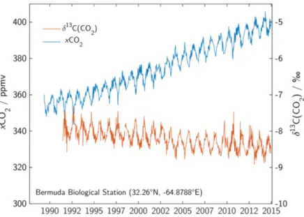
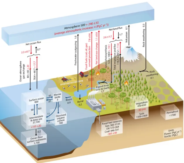
Since the rst observation of a rising carbon dioxide (CO2) content in the atmosphere (Keeling, 1960), the Earth's carbon cycle has received particular attention. Under- standing which exact processes are forcing this increase and which have the potential to weaken it has become one of the major tasks of humankind. Since the start of the industrialization in the 18th century, the carbon content in the atmosphere rose from xCO₂ = 279ppmv to currently (January 2016) xCO₂ = 402.59ppmv (Dlugokencky and Tans, 2016). The increase during the last decades from 355 ppmv to about 400 ppmv and the simultaneous decrease in its stable carbon isotope ratio at the atmospheric measurement site in Bermuda (32.26^◦N, -64.88^◦E) is shown in Figure 1.1. This increase is caused by the combustion of fossil fuels and emissions due to land use changes which are both mediated by the ongoing industrialization as conrmed through the isotope measurements. The annual variability of CO2 and its stable carbon isotope ratio is mostly driven by changes in land biomass which reduces the atmospheric carbon content towards a minimum in CO2 in late summer. The rising CO2 in the atmosphere is only accounting for about half of the carbon that was released via fossil fuel combustion and land use changes. The other half is stored in the ocean and in vegetation and soils. The amount of carbon stored in land vegetation and soils is usually calculated as the dierence between sources, remaining carbon in the atmosphere and the ocean sink (Le Quéré et al., 2015). In this approach, a better estimation of the ocean carbon sink subsequently reduces the uncertainty in the land carbon sink. Figure 1.2 shows a schematic overview of the Earth's carbon cycle. The major part of the oceanic carbon is stored in the intermediate and deep sea. The surface ocean as relative small carbon reservoir is the only connection between the deep ocean and atmosphere.

The magnitude of the ocean carbon sink, however, is highly variable and strongly depending on region, wind conditions, and the dierence between atmospheric and surface ocean CO2 partial pressure. The North Atlantic plays a major role when it comes to quantifying the oceanic carbon sink. Here, one of the highest uptake rates of CO2 was

1

(20)

Figure 1.1: Atmospheric CO2 concentrations and its stable carbon isotope ratio at Bermuda (data taken from "Cooperative Global Atmospheric Data Integra- tion Project" (2015) and White et al. (2015)).

detected ((2.2±0.7)molC m⁻²yr⁻¹, (Takahashi et al., 2009; Ciais et al., 2013)). This high uptake rate is mostly driven by a large disequilibrium during the spring and summer period. For a better quantication of the North Atlantic carbon sink and a prediction of its future changes it is necessary to understand the underlying processes. When and why does the spring bloom start? How fast is biomass growing? What is supporting this growth and what slows it down? When does it run into nutrient limitation? Which role does the community structure of phytoplankton play (i.e., calcifying vs. non-calcifying phytoplankton)? How many nutrients are remineralized at which depth? Which inuence has the the maximum winter depth for the nutrient budget and, consequently, the productivity of the following productive season? How does this picture change spatially, but also in response to interannual climate variability or long term processes such as climate change? Many scientists are working towards nding answers to these questions by doing eld measurements, lab experiments or model studies. In addition, much eort is being made to improve the understanding of the gas exchange velocity and its relationship with the wind or an organic microlayer covering the surface ocean (Wanninkhof et al., 2009).

Another approach considers the establishment of a widespread observation system for

(21)

Chapter 1. Introduction 3

Figure 1.2: The global carbon cycle and the size of its reservoirs and annual uxes.

Black numbers denote the preindustrial conditions and red numbers account for the respective anthropogenic inuences as average over the years 2000- 2009. Arrows show the annual uxes between dierent reservoirs (Ciais et al., 2013).

(22)

Figure 1.3: Net the air-to-sea CO2 ux as estimated from surface ocean pCO2 measurements (Takahashi et al., 2009).

CO2 dynamics in the surface ocean. Using commercial ships for investigating ocean and atmosphere is a relatively ecient method that has already been used for meteorological measurements and monitoring changes in plankton abundances (Reid et al., 2003). Since the possibility of autonomous measurements of surface water CO2 was developed, a network of Voluntary Observing Ships (VOS) has been established and equipped with measurement systems for CO2 partial pressure (pCO2). The data from this network has been combined, quality controlled and provided the basis for calculating a climatology of seawaterpCO2 and the corresponding annual air-to-sea uxes (Takahashi et al., 2009;

Watson et al., 2009). Up until now, this data compilation is continuously growing and provides the possibility to have a look on interannual variations in the air-to-sea CO2

ux (Bakker et al., 2014; Landschützer et al., 2014).

MeasuringpCO2 alone, however, does not give a complete picture. Consistent datasets

(23)

Chapter 1. Introduction 5 have also been developed for other relevant parameters such as the total dissolved inorganic carbon (DIC), total alkalinity (TA), nutrients and the stable carbon isotope ratio of DIC δ¹³C(DIC) (Olsen et al., 2016; Becker et al., 2016). Isotope measurements can improve the understanding of complex systems since each process has a dierent im- pact on the respective isotopomers. The measurement of stable carbon isotopes in DIC, for example, has been used as tracer for net community production and anthropogenic carbon (Körtzinger et al., 2003; Quay et al., 2009). However, the applicability of this parameter was always limited due to an insucient temporal and spatial data resolution.

With the ongoing development of high resolution spectrometric methods, new measuring systems became available. Robust and sensitive cavity ringdown analyzer provide the possibility of autonomous isotope measurements directly onboard a vessel. By com- bining these instruments with the VOS network, the spatial and temporal resolution of isotope data can be signicantly improved.

The aim of this work is to draw a full picture of surface ocean carbon and nutrient dynamics in the North Atlantic. Therefore, full annual cycles of stable carbon isotope ratio of surface water CO2 have been measured on a VOS sailing routinely between Liverpool, UK and Halifax, Canada. The changes in the stable carbon isotope ratio were compared to continuous measurements of the fugacity of carbon dioxide (fCO2) and discrete samples of inorganic and organic carbon parameter and nutrients. By setting up a small box model, the seasonal inuences of air-sea gas exchange, net community production and convective mixing on the carbon and nutrient cycles in surface water have been calculated.

At rst, an internally consistent dataset of the stable carbon isotope ratio of DIC in the North Atlantic Ocean is presented (Chapter 4). In Chapter 5, the obtained underway data of surface ocean fCO2 and its stable carbon isotope ratio (δ¹³C(CO2)) from 2012 to 2015 will be presented and its interannual variability will be interpreted. Chapter 6 describes the outcome of a simple box model and the magnitude of air-sea gas exchange, net community production and convective mixing across the North Atlantic. In the following, the seasonal changes in seawater fCO2 andδ¹³C(CO2), DIC, δ¹³C(DIC), TA, chlorophyll a, particulate and dissolved organic matter, nitrate, phosphate, silicate and nitrite will be discussed. The stoichiometric composition of the produced particulate matter and the relative consumption of DIC, nitrate, phosphate and silicate will be addressed in Chapter 8. Eventually, some insight into the variability of stable isotopes in particulate carbon and nitrogen (δ¹³C(POC) and δ¹⁵N(PON)) and the fractionation

(24)

(25)

2 Scientic background

2.1 Properties of the North Atlantic Ocean

The study region, the North Atlantic between 40 and 60^◦N, shows both, subpolar and subtropical inuences. According to Longhurst (2007) the surface water can be divided into dierent biogeographical provinces of comparable ecology, the Gulf Stream province (GFST), the Northwest Atlantic Shelves (NWCS) and the North Atlantic Drift (NADR).

The mean surface velocity and ow direction for the years 2012-2014 for this region as well as the provinces are shown in Figure 2.1.

The GFST province is located in the western part and characterized by warm and saline water masses that are transported northeastwards by the 'Gulf Stream'. The Gulf Stream forms in the Gulf of Mexico, follows north the American coast and nally turns east into the North Atlantic. The position at which it leaves the coast as well as its strength is varying slightly during the year, with the northernmost position occurring in fall and a more southward position in winter and early spring (Auer, 1987; Frankignoul et al., 2001). The water transport is highest in fall and lowest in spring (Zlotnicki, 1991;

Hogg and Johns, 1995). The Gulf Stream shows a signicant meandering which changes from a single branch to multiple fronts once it reaches the Grand Banks and shows a high amount of eddy activity. Here it meets the western boundary current of the subpolar gyre, the Labrador Current, which transports cold and relatively fresh water out of the Labrador Sea and forms at the front a region with high kinetic energy. At any time of the year cold, cyclonic eddies at the seaward side of the front and warm, anticyclonic eddies on the shore side can be observed. These eddies can be 1000 −3000m deep and 100−300km wide (Frankignoul et al., 2001). The cold water side is representing the northern part of the NWCS province which covers the entire US coast between the Florida Keys and the Street of Belle Isle.

The continuation of the northward branch of the Gulf Stream which is intensied by mixing with the Labrador Current, is the North Atlantic Current (NAC). Most of it

7

(26)

Figure 2.1: Mean surface currents from 2012-2014 and the Longurst. The arrows indicate the velocity and the ow direction (red: eastwards, blue: westwards) (Bonjean and Lagerloef, 2002). According to Longhurst (2007) the dierent biogeographical provinces are shown (NWCS: Northwest Atlantic Shelf, GFST: Gulf Stream, ARCT: Atlantic Arctic, NADR: North Atlantic Drift, NAST(E): Northeast Atlantic subtropical gyre).

ows north until about 52^◦N, forms a loop and then turns east (Krauss et al., 1987).

The other part of the NAC ows directly in northeastern direction. Around 30^◦W the NAC turns into the North Atlantic Drift Current (NADC) which is slowly moving northeastwards, feeding the currents of the Nordic Seas. The southern boundary of the NADC is formed by the eastwards owing southern branch of the NAC which is the northern part of the subtropical gyre.

It could be seen that climate variations such as the North Atlantic Oscillation (NAO) can induce latitudinal variations of the Gulf Stream and can inuence the timing of the spring bloom (Henson et al., 2009b) as well as the abundance of certain plankton species (Hays et al., 1993; Borkman and Smayda, 2009). The mostly wind driven NADC is also inuenced by changing wind patterns, which themselves depend on the NAO (Bigg

(27)

Chapter 2. Scientic background 9 et al., 2005).

The biological seasonality of the sampling region is mainly driven by deep convection in winter time which transports nutrients to the surface and a distinct spring bloom during which the nutrients are more or less completely depleted. In the western part, where the winter convection is not as deep, eddies and turbulence at the front of Labrador Cur- rent and Gulf Stream play a signicant role in nutrient supply. The onset of the spring bloom can vary by one month between the south and the north of the sampling area but has been shown to start way before a complete stratication is reached (Colebrook, 1982). For the eastern North Atlantic it was observed that rst a diatom-dominated bloom is developing, which then is followed by agellates after silicate depletion has occurred (Sieracki et al., 1993; Lochte et al., 1993). Data from Continuous Plankton Recorder (CPR) measurements indicate a southwards decreasing spring bloom intensity and increasing fall bloom intensity (Colebrook, 1979). In the frontal region of the Labrador Current and Gulf Stream the stratication develops earlier than in the surrounding water masses. Due to this fact and a continuous nutrient supply by upwelling the bloom can persist longer and intensied (Ferrari et al., 2015). In the eastern part of the North Atlantic, also a small bloom in fall can be observed. The extent to which nutrients are depleted at the end of spring bloom and deepening of the mixed layer can trigger a bloom at the end of the summer is increasing towards the south (Chiswell et al., 2015).

The composition of biomass in the ocean follows a relatively xed stoichiometric ratio of C:N:P = 106:16:1, the so called Redeld ratio (Redeld, 1958). However, this is only a mean value and the composition of newly produced phytoplankton biomass can deviate widely from this ratio (Körtzinger et al., 2001). This can happen by processes such as nitrogen xation and denitrication (Gruber and Deutsch, 2014), or a shift in internal lipid structure from phospholipids to other lipids under phosphate limitation (Geider and Roche, 2002). Moreover, dierent responses to nutrient limitation combined with species shifts as well as dierent measurement techniques lead to a wide range of reported element ratios for ocean biomass (Koeve, 2006).

2.2 Carbonate system

Inorganic carbon in the ocean can appear in several dierent forms. When atmospheric CO2 dissolves in the ocean (CO2,aq) it can react with water by forming true carbonic

(28)

(CO²⁻₃ ). For describing the speciation of dissolved inorganic carbon in the ocean, the entire inorganic carbon system has to be taken into account. The two electrically neutral forms of dissolved CO2 are usually combined and here denoted by CO2. The following equilibria govern the marine CO2 system.

CO_2,g ^K*)⁰ CO₂ (2.1)

CO₂+ 2 H₂O^K*)¹ HCO⁻₃ + H₃O⁺ (2.2) HCO⁻₃ + H₂O^K*)² CO²⁻₃ + H₃O⁺ (2.3) Here, K0 is the Henry constant for carbon dioxide in seawater and K1 and K2 the dissociation constants of carbonic acid in seawater. Please note, that all constants used in this thesis are related to the respective concentrations and not activities in seawater.

Because of that, they depend on temperature, salinity and pressure (Mehrbach et al., 1973; Lueker et al., 2000; Millero et al., 2002).

In typical seawater at a pH around 8, bicarbonate is the dominant species ([HCO⁻₃] : [CO²⁻₃ ] : [CO2] ' 86.5% : 13% : 0.5%)(Zeebe and Wolf-Gladrow, 2005). The variations within the CO2 system are usually described by four dierent parameters, fugacity of carbon dioxide (f CO2), pH, total alkalinity (TA), and total dissolved inorganic carbon (DIC). By knowing two of these, the other two can be calculated.

Parameters describing the carbonate system

The amount of carbon dioxide in seawater is usually expressed as fugacity (f CO2) or partial pressure (pCO2) of carbon dioxide in a gas phase that is in equilibrium with the seawater. The fugacity considers also the non-ideal behavior of CO2in air and, therefore, is the more accurate parameter. It can be determined from the equation of state.

ln

fCO₂ p

= ln (xCO₂)− × 1 RT

Z p 0

RT

p −V_m(p)

dp (2.4)

wherepis the pressure,xCO2 the mole fraction, V_mthe molar volume of carbon dioxide, R the gas constant and T the absolute temperature. A good approximation for real gases is given by an empirical power series expansion, the virial equation (Eq. 2.5).

pV_m

RT = B(x, T)

V_m + C(x, T)

V_m² +... (2.5)

(29)

Chapter 2. Scientic background 11 where B and C are called virial coecients and both are functions of temperature.

Neglecting higher order terms leads to a simple expression for the fugacity of pure CO2

by inserting Eq. 2.5 in Eq. 2.4:

fCO₂ = xCO₂×p exp

B_CO₂ V_m

(2.6) The second virial coecient B_CO₂ considers the interactions between two molecules of the same type. When investigating a gas mixture, the cross-virial coecient δ_CO₂ has to be taken into account, which considers the interactions between molecules of dierent type (Guggenheim, 1950).

The pH is the negative common logarithm of the H⁺-ion concentration and, therefore, represents the thermodynamic state of all acid-base-systems in the seawater. In the marine environment it is reported in three dierent scales (total scale, seawater scale, and free scale). They depend on dierent consideration of protonated species of sulphate and uoride ions and can be converted among each other.

The alkalinity is related to the charge balance of seawater. It is dened as the number of moles of hydrogen ion equivalent to the excess of proton acceptors over proton donors in one kilogram of sample.(Dickson, 1992; Wolf-Gladrow et al., 2007)

TA =

HCO⁻₃ + 2

CO²⁻₃ +

B (OH)⁻₄ +

OH⁻ +

HPO²⁻₄ + 2

PO³⁻₄ +

H₃SiO₄⁻

+ [NH₃] + HS⁻

− H⁺

F −

HSO⁻₄

− [HF] − [H3PO4]

(2.7)

with [H⁺]_F referring to the free pH-scale.

The dissolved inorganic carbon represents the mass balance of the carbon system as it is the sum of the concentrations of all dissolved inorganic carbon species.

[DIC] = [CO2] +

HCO⁻₃ +

CO²⁻₃

(2.8) Processes driving the carbonate system

Processes inuencing the oceanic carbonate system such as air-sea gas exchange of CO2, primary production or calcication inuence these four carbon parameter in a dierent way. Figure 2.2 shows these dierent inuences as a function of DIC and TA.

At dierent depths in the ocean dierent processes are important. At the surface CO2

can enter the ocean from the atmosphere, resulting in increasing the DIC concentration and decreasing the pH. The outgassing of CO2 into the atmosphere has opposite eects.

(30)

Figure 2.2: Eects of dierent processes (air-sea gas exchange, photosynthesis, respiration, dissolution and formation of CaCO3) on the carbon system parameters in the ocean. The solid and dashed contours indicate dierent levels of CO2

concentrations and pH as a function of DIC and TA, respectively. The arrows show the respective inuence of each process on DIC, TA, pCO2 and pH (Zeebe and Wolf-Gladrow, 2005).

The production of biomass leads to a decrease in DIC concentration and a small increase of TA due to the consumption of other nutrients such as nitrate and a concurrent uptake of H⁺.

The air-sea gas exchange is driven by the fugacity dierence of CO2 between the atmosphere (fCO_2,ATM) and the ocean (fCO_2,_SEA). The atmospheric f CO2 undergoes only relatively small changes throughout the year since it is well mixed. In contrast to that, the oceanic f CO2 can show a higher variability caused by the contribution of various physical, biological and chemical processes such as temperature changes, verti- cal and horizontal mixing, air-sea gas exchange or primary production. However, the actual exchange ux between ocean and atmosphere is limited by the turbulence at the

(31)

Chapter 2. Scientic background 13 interface. The ux between atmosphere and ocean is expressed as

F_CO₂ =k×K₀×(fCO_2,_ATM−fCO_2,_SEA) (2.9) where K₀ is the solubility of CO2 in seawater (Weiss, 1974) and k the gas transfer velocity. The gas transfer velocity is commonly related to wind speed (Wanninkhof, 1992; Wanninkhof et al., 2009; Nightingale et al., 2000) but is also be eected by waves, bubbles or surfactants which can lead to deviations from the wind speed relationship especially under intense bloom conditions with a high surfactant concentration.

The exchange of CO2 between the surface ocean and deeper water masses is driven by dierent biologically or physically driven pumps. The 'solubility pump', or 'physical pump' transports the CO2 by subduction of water masses and convective mixing.

Biological processes are divided due to their dierent inuences on the carbon system (see Figure 2.2) into the 'soft tissue pump' and the 'hard tissue pump'. The 'soft tissue pump' (also 'organic carbon pump') represents the production of particulate organic carbon in the productive area which partly sinks to deeper water masses where it is remineralized and released in the form of CO2. This process removes xed carbon from the air-sea interface and therefore reduces the CO2 concentration at the surface. The 'hard tissue pump' is based on the formation of particulate inorganic carbon, mainly calcium carbonate, which then sinks into the deep ocean, where it can be either buried or dissolved. In contrast to the soft tissue pump the biological production of calcium carbonate leads to an increase of CO2 concentrations in the productive zone.

Ca²⁺+ 2 HCO⁻₃ *)CaCO₃+ CO₂+ H₂O (2.10)

2.3 Stable isotopes of carbon and nitrogen

The dierent abundances of stable isotopes in chemical substances give us the possibility to distinguish between dierent biological and physical processes such as biological uptake, remineralization, air-sea gas exchange or fossil fuel burning.

The isotope composition of a material concerning a given element is usually described as the molar ratio of the heavier to the lighter isotope, ^νR, with νh being the mass number of the heavier isotope and ν_l the mass number of the lighter isotope. For the

(32)

ν_h

R =

ν_hC

ν_lC =

13C

12C (2.11)

The common expression to report isotopic abundances in environmental science is the δ notation. For this, the isotopic ratio of the sample substance is expressed as per mil deviation from that of a reference material.

δ^ν = _ν

R_sample

νR_reference −1

×10³ (2.12)

For carbon, this reference material is Pee-Dee-Belemnite (PDB) with a molar ratio of ¹³R_PDB = 0.0112372(±3) (Craig, 1957). This reference substance stems originally from a limestone from a marine fossil, Belemnitella americana, sampled at the Pee Dee formation in South Carolina, USA. However, caused by the limited availability of this today articial standard materials such as Vienna Pee-Dee-Belimnite (V-PDB) are used.

For nitrogen, atmospheric nitrogen is used as reference material.

Most chemical reactions or phase transitions alter the isotopic ratio of a substance which is called fractionation. The fractionation between two chemical or physical states A and B can the expressed by the fractionation factor ^να(A−B).

να(A−B) =

νR_A

νR_B (2.13)

Since changes in biological isotope distribution are usually very small, the fractionation factor can also be expressed in h according to the δ notation.

ν_(A−B) = _ν

R_A

νRB −1

×10³ (2.14)

Providing that α is close to unity, can be approximated by the dierence of the δ¹³C values of the two species:

(A−B)= δ_A^ν −δ_B^ν

1 +δ^ν_B×10⁻³ ≈δ^ν_A−δ_B^ν (2.15)

Fractionation Processes

With most changes in the chemical or physical state of a substance comes an isotopic fractionation. This is caused by the dierent mass of both isotopomers which induces small dierences in their chemical and physical behavior. The fractionation processes can

(33)

Chapter 2. Scientic background 15 be divided into chemical and physical kinetic fractionation which occur during incomplete transformations of transport processes and equilibrium fractionation at a chemical or physical equilibrium.

The fractionation in a thermodynamically equilibrated system, e.g. the reactions of the inorganic carbon species in the ocean or, more or less, the air-sea gas exchange, is called equilibrium fractionation. This fractionation is a consequence of dierent zero-point energies of both isotopomers at each side of the equilibrium. The dierence between the zero-point energies of the two isotopomers is increasing with increasing zero-point energies, or, in other words, is larger the stronger this element is bound in the molecule.

This leads for example to an enrichment of ¹³C in bicarbonate and carbonate relative to carbon dioxide.

During incomplete reactions or transport processes kinetic fractionation can occur.

The chemical kinetic fractionation arises from the mass dependence of reaction rates. It occurs only during incomplete reactions or when the product of the reaction is removed from the system. Basically all isotope eects during biological uptake and remineralization are kinetic. The reaction of the lighter isotopomer is usually slightly faster which comes from a smaller dierence of the zero-point energies of the reactant and the tran- sition state. The magnitude of the fractionation is determined by the ratio of the rate constants of the two isotopomers.

Physical kinetic fractionation occurs for example during diusion processes or phase transitions. During diusion the fractionation occurs because of the mass dependence of a molecules mobility. For two isotopomers having the same kinetic energy, the lighter molecule moves faster and, thus, has a higher diusion coecient. The fractionation is then given by the ratio of both diusion coecients.

The eect of kinetic fractionation while material is removed from the system is called Rayleigh process. This fractionation occurs, for example, during the assimilation of nutrients during phytoplankton growth. During a kinetic fractionation process the remaining reactant gets continuously enriched in the heavier isotopomer. With a constant fractionation factor this leads to a constant increase of the instantaneous isotope ratio in the product. When the reaction is complete no net fractionation between the reactant and the accumulated product remains. The isotope ratio of the residual reactant (^νR_res) can be calculated using the fractionation factorα, the fraction f of the remaining

(34)

Figure 2.3: Rayleigh fractionation process during primary production from nitrate (left hand) and DIC (right hand). The change in the abundance of ¹⁵N (δ¹⁵N) is shown for nitrate, the accumulated biomass and the instantaneous produced biomass with a fractionation between nitrate and biomass of ( = −5h).

When the nitrate is consumed completely (f =0), the accumulated biomass has the same isotopic signature as the initial nitrate. The same is also shown for the change in¹³C of DIC and biomass, respectively (δ¹³C). For the fractionation between DIC and organic matter a constant value of=−24h was used.

reactant and the isotope ratio (^νR0)at t= 0:

νR_res =f^(α−1)×^ν R₀ (2.16)

From this, the instantaneous isotope ratio of the product^νR_inst follows as:

νR_inst =α×f^(α−1)×^ν R₀ (2.17)

Finally, the isotope ratio of the accumulated product^νRacc can be calculated as:

νR_acc = f^α−1

f−1 ×^ν R₀ (2.18)

For the consumption of nitrate and DIC by phytoplankton the development of the dif- ferent isotope ratios of ¹⁵N and ¹³C is shown in Figure 2.3. For nitrogen isotopes in the ocean this process is very important because the reservoir of inorganic nitrogen can be

(35)

Chapter 2. Scientic background 17 completely consumed during bloom events. A sucient change in the DIC pool to alter the isotopic composition in a signicant way only occurs during very intense blooms.

Natural abundance and fractionation in the marine carbon system

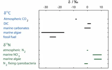
The abundance of stable isotopes in the environment can vary a lot along the dierent components and processes. The stable carbon isotope ratio in materials that are important for the marine carbon cycle are shown in Figure 2.4. In preindustrial times, the atmosphere had a stable carbon isotope ratio of about −6.3h (Tagliabue and Bopp, 2008). The combustion of fossil fuels since the beginning of the industrial revolution, which reveal the relative lowδ¹³C value of their biological origin (about−23h), leads to a continuous lightening of the atmospheric carbon along the increase of carbon dioxide in the atmosphere to values below−8h today (Keeling et al., 1995). This decrease was rst recorded by H. Suess and is called ¹³C Suess eect (Keeling, 1979). Caused by the equilibration processes between atmosphere and ocean, the lightening of atmospheric carbon can also be observed in the marine inorganic carbon, here known as oceanic Suess eect. The DIC is changing by about (−0.24 ± 0.02)h per decade (Quay et al., 2003; Körtzinger et al., 2003). The typical δ¹³C of DIC in the ocean lies between 0h and 2h (Quay et al., 2003). However, during intense bloom events these values can be clearly exceeded. This increase is a result of the fractionation that is occurring during biological carbon xation. The isotopic composition of organic carbon in plants varies between −32h and −22h depending on the exact mechanism of carbon xation and other eects such as the temperature dependence of fractionation. Marine carbonates such as the CaCO3 shells of coccolithophores show an isotopic signature close to that of DIC.

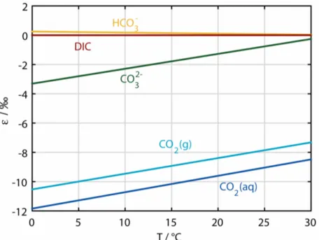
The fractionation within the marine carbonate system can be described by equilibrium fractionation. Since an equilibrium reaction can be divided into reactions of ¹³C and ¹²C and the fractionation factor can be described using the equilibrium constants, this fractionation factor is temperature and salinity dependent. Moreover, some metal ions who are capable of building carbonate complexes in seawater, such as Mg²⁺, can inuence the fractionation factors in natural seawater compared to those determined in articial seawater. Unfortunately, there are only a few studies available that focus on the fractionation between DIC and the dierent carbon species in seawater. Besides temperature and salinity, the overall fractionation between DIC and gaseous CO2 depends also on the relative abundance of the dierent species inside the carbon system and,

(36)

Figure 2.4: Isotopic composition of carbon and nitrogen in selected materials (redrawn after Zeebe and Wolf-Gladrow (2005); Ohkouchi et al. (2015); Sigman et al.

(2009)).

thus, on the pH. The fractionation factors used in this work (Zhang et al., 1995) and the temperature dependence of the fractionation between the various inorganic carbon species are shown in Table 2.1 and Figure 2.5.

The autotrophic xation of inorganic carbon is a non-equilibrium process causing kinetic fractionation. Besides the temperature and salinity dependence, this reaction is also dependent on the pathway over which the marine phytoplankton produces its organic matter. This 2-step process can vary with the availability of carbon dioxide and nutrients and the growth rate. Usually, the carbon dioxide diuses through the cell membrane into the cell, where it reacts with the enzyme RubisCO as the rst step in the formation of organic matter. The rst, diusive process is a reversible equilibrium process, whereas the enzymatic reaction is irreversible. The decreasing CO2

concentrations in the surrounding water or a high growth rate of the cell can limit the availability of carbon dioxide inside the cell and, therefore, turn the transport into the cell to being the rate determining step. In this case, the cell can activate an active transport mechanism of bicarbonate ions into the cell. The use of bicarbonate instead of carbon dioxide leads to an increased abundance of the heavier isotope in the produced organic matter caused by the higher isotope ratio of bicarbonate compared with dissolved carbon dioxide. At which level a cell activates this active transport and to which portion bicarbonate is used, is, of course, also dependent on the species. It is shown, that the

(37)

Chapter 2. Scientic background 19

Figure 2.5: Temperature dependence of the carbon isotope fractionation between the species of the carbonate system and total dissolved inorganic carbon (DIC) (at pH=8.15) (redrawn after Zhang et al. (1995)).

fractionation of the overall carbon xation _p correlates negatively with the growth rate, which itself is controlled by external parameters such as nutrient supply, temperature and light intensity (Takahashi et al., 1993). The more the mass transport process is the limiting process and the carboxylation happens quantitatively, the less negative the produced organic matter will be because the diusion process induces a relatively small fractionation. The complete remineralization of organic matter is a quantitative process, leading to a release of inorganic carbon with the same isotopic signature as the organic matter.

Natural abundance and fractionation in the marine nitrogen system

Since inorganic nitrogen exists in more chemical forms in the ocean than inorganic carbon, the fractionation processes of these species among each other as well as with organic matter are more complicated. Unfortunately, the database for estimating these inuences is rudimentary. Here, I will concentrate on processes that are relevant for the North Atlantic surface ocean. The abundances are shown in Figure 2.4. The dissolved N2 is slightly enriched in ¹⁵N compared to gaseous nitrogen (Ohkouchi et al., 2015).

When organic matter is produced from this nitrogen reservoir by N2-xation the pro-

(38)

Table 2.1: Fractionation factors within the carbon system and their temperature dependence (in ^◦C).

Process /h

CO2 invasion (as) −0.013×TC−2.30

(Zhang et al., 1995)

CO2 - CO2(g) +0.0049×TC−1.31

HCO⁻3 - CO2(g) −0.1141×TC+ 10.78

CO²⁻3 - CO2(g) −0.0052×TC+ 7.22

DIC - CO2(g) −0.107×TC+ 10.53 + 0.014×TC×f(CO²₃⁻) (Zhang et al., 1995)

Diusion 0.7 - 0.9

(O'Leary, 1984; Jähne et al., 1987)

Carboxylation 18 - 30

(Chikaraishi, 2014)

duced organic nitrogen has an isotope signature of−2to0h (Hoering and Ford, 1960;

Minagawa and Wada, 1986). Nitrate has an average isotope ratio of 5h and is usually enriched in the photic zone due to primary production (Sigman et al., 2009). The fractionation during the nitrate assimilation of phytoplankton is about 5h. Since the nitrogen can be fully depleted during the spring bloom, the Rayleigh process has a large inuence on the isotopic composition of nitrate and the produced organic nitrogen (see Figure 2.3). Also for nitrate, the growth rate can have a large inuence on the isotopic fractionation associated with nitrate assimilation (Wada and Hattori, 1978).

2.4 Cavity Ringdown Spectroscopy

Cavity Ringdown Spectroscopy is a technique for highly accurate concentration measurements in the gas phase. The increased accuracy with respect to simple absorption techniques is based on two main factors. Using a stable optical cavity with two or more highly reective mirrors (R > 99.99 %) leads to long path-lengths of light up to several kilometers which results in an increased sensitivity of the absorption measurement.

Moreover, unlike most other absorption-based methods, this technique determines the

(39)

Chapter 2. Scientic background 21

Figure 2.6: Basic setup of a CRDS experiment ("Picarro Inc.").

concentration of the target gas in the cavity by measuring the time constant of the loss of light intensity within the cavity. In the most simple setup for a CRDS experiment, a pulsed laser is coupled into a resonant optical cavity and for each laser pulse the decay time of the light intensity inside the cavity is determined by detecting the small intensity fraction leaking through the mirrors with a photodetector. This 1/e decay time τ is given by:

τ(ν) = t_r

2 (1−R) + 2α(ν) L (2.19) with t_r being the roundtrip time of the light within the cavity, α(ν) the absorption coecient for frequency ν, and L the cavity length. The dominant factor for the decay time of an empty cavityτ₀ is the reectivity of the mirrors. In the presence of an absorber inside the cavity, the observed decay time of the intensity decreases. By knowing the absorption coecient at the concrete wavelength, the concentration of the absorber can be determined from the dierence between this decay time τ and τ₀.

c= 1 α(ν)

1 τ − 1

τ0

(2.20)

(40)

complex setup (see Figure 2.6). Here, the laser beam intensity is built up in the cavity only when the laser wavelength matches the resonance frequency of a cavity mode.

Mostly, this is achieved by moving one of the mirrors with a piezoelectric transducer (PZT). Once the laser is switched o the ringdown can be detected.

(41)

3 Experimental

3.1 Precise measurements of xCO

²

and δ

¹³

C(CO

²

) using CRDS

The CRDS measurements were performed using a commercial analyzer (G2131 i, Picarro, USA). In this instrument a tunable cw-diode laser with a narrow bandwidth and an emission maximum around 1600 nm is used to determine ¹²CO2, ¹³CO2, H2O and CH4

in air. The absorption spectrum of ¹²CO2 and ¹³CO2 which was scanned with a scan increment of 0.02 cm⁻¹ is shown in Figure 3.1. The sample gas was pumped through a 3-mirror cavity by an external pump with a ow rate of about 20 mL min⁻¹. Inside the cavity, the pressure was held constant at (140.00±0.07) torr, ((186.60±0.09) mbar), by controlling the gas ow via the inlet valve, and the temperature was locked at (45.00± 0.02)^◦C. The precisions of cavity pressure and temperature were the determined in the laboratory. At sea, the instrument's performance was slightly reduced, most likely due to small pressure instabilities, which were induced by the vessels vibration. The analyzer used peak heights, tted with a Galatry line prole, instead of peak integrals to determine the sample's concentrations. This leads to a strong dependence of the measured concentration on the cavity pressure and the sample gas composition since both eect the pressure broadening of absorption lines. The analyzer was calibrated for measuring atmospheric gas and, therefore, the oxygen content was the only compound changing the gas composition. Its concentration was determined using the Galatry broadening parameteryfrom the analyzers t routine and the isotope ratio was corrected by an O2-calibration curve as described in Friedrichs et al. (2010) and Becker et al.

(2012). The δ¹³C(CO2) was calculated from x¹²CO2 and x¹³CO2 which were corrected for inuences of H2O and CH4 by internal calculation routines. An 'Allan deviation analysis' was performed for determining the precision of the analyzer and the optimal averaging time for maximal improvement of the signal to noise ratio. The Allan variance

23

(42)

Figure 3.1: The measured absorption spectrum of ¹²CO2 (6251.76 cm⁻¹) and ¹³CO2

(6250.42 cm⁻¹) (van Pelt, 2008).

σAllan is dened as the average variance of two adjacent averages of a time series. In an optimal system with only statistical noise, longer averaging time would always lead to a higher precision. In reality, however, long term drifts of the instrument lead to an increase in the Allan variance. The minimum of the Allan plot (σ_Allanvs. averaging time τ) indicates the optimal averaging time. The result of this analysis for the δ¹³C(CO2) is shown in Figure 3.2. The optimal averaging time is found to be τ = 150min yielding a precision of 0.09h, determined at xCO2 = 348.06ppmv. At higher xCO2, the precision of the δ¹³C(CO2) measurements is improved due to a better signal-to-noise ratio.

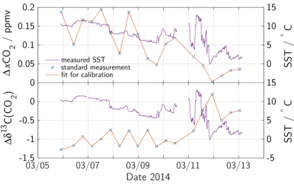
Despite the precise temperature locking inside the cavity, the analyzer showed a strong dependence on room temperature in its measured isotope ratio as well as small inuences on the measured CO2 partial pressure. This temperature dependence is assumed to be caused by a temperature dependence of the mirror reectivity. This eect and the dependence of the measured isotope ratio on absolute xCO2 are taken care of by reg- ular measurements of two dierent standard gases. The measurements were corrected towards these standard measurements by linear regression in time and xCO2. As an example, the development of the standard gas measurements (at xCO2 = 348.06ppmv, δ¹³C(CO2) = −3.28h) during the westbound crossing COM 14-04 is shown in Fig- ure 3.3. The colder room temperatures caused by colder seawater temperatures in the

(43)

Chapter 3. Experimental 25

Figure 3.2: The Allan deviation of calibration gas measurements of δ¹³C(CO2) at xCO2

= 348.06 ppmv.

last days of the crossing lead to higher isotope ratios and smaller xCO2 which are corrected by linear regression between two standard measurements.

3.2 Underway measurements and data reduction of f CO

²

and δ

¹³

C(CO

²

)

The data used in this study were recorded on the 'Voluntary Observing ship' (VOS) M/V Atlantic Companion (Atlantic Container Lines (ACL), New Jersey, USA), which was operating on a transatlantic route between Liverpool, UK and Halifax, Canada. The measurements used in this study were performed between January 2012 and December 2014. The extensive sampling program comprised continuous underway measurements of fCO2 andδ¹³C(CO2) in seawater and air and discrete samples of DIC, TA, Chl a, POM, DOM, nitrate, phosphate, silicate, nitrite, δ¹³C(POC) andδ¹⁵N(PON). The tracks of the crossings and the sampling locations are shown in Figure 3.4. Whether the vessel passed Ireland on a northern or southern route was dependent on the location of the major low pressure systems, which the vessel tried to avoid, and had no seasonal pattern. In contrast to that, there was a small seasonal variation in the vessel tracks at the western

(44)

Figure 3.3: Development of standard gas measurements of xCO2 (upper plot) and δ¹³C(CO2) (lower plot) during the westbound crossing COM 14-04 at a xCO2

of 348.06 ppmv. For comparison, the measured SST is also shown.

side of the basin (west of 50^◦). Caused by the more southward extent of the ice border o the coast of Newfoundland in late spring and early summer, the vessel sailed more south at this time of the year, especially during 2014.

The underway unit was located in the engine room of the vessel. A schematic setup is presented in Figure 3.5. An autonomous pCO2 measuring system as described in Lüger et al. (2004) and Steinho et al. (2010) was connected to a sea chest on port side, that was located about 250 m astern of the forecastle. On average, its water inlet was located at a depth of 9.6 m during eastbound and 10.6 m during westbound crossings as given by the vessel's draft. Directly after the water inlet the sea water temperature was measured by an external temperature sensor (SBE 38, accuracy of ≈0.01^◦C). To prevent biofouling and oxygen consumption inside the pipes, the water passed a copper electrode before it was pumped to the measuring system by a torque-ow pump. Prior to entering the pCO2

measuring system, the salinity was measured by a Seabird thermosalinograph SBE 21 (accuracy: SSS: ≈ 0.1psu, equilibrator temperature ≈ 0.01^◦C). The pipe length from the sea chest to the pCO2 measuring system was about 4 m and the water ow rate was

(45)

Figure 3.4: Vessel tracks of M/V Atlantic Companion and the sampling positions of underway measurements (upper panel) and discrete samples (lower panel).

The location of the four boxes used in the further analysis is also illus- trated. The three dierent years are denoted with dierent colors (2012:

light blue/circles, 2013: mid blue/triangles, 2014: dark blue/crosses).

controlled to be at 2-3 L min⁻¹. In the pCO2 measuring system, a NDIR CO2 analyzer (Licor 7000) was used. Downstream of the Licor, the CRDS was installed as a bypass.

The gas outlet of the CRDS was redirected to the main gas ow. The CRDS pump was sealed so that its leakage was small enough to not inuence the equilibration (Becker et al., 2012). The response time of the equilibrator to rapid changes in fCO2 was about 2 min (Pierrot et al., 2009). The CRD analyzer was calibrated every 8 - 10 h using two standard gases with dierent CO2 concentrations. Atmospheric air was also measured every 8 - 10 h. During crossings without CRDS measurements, the NDIR analyzer was calibrated every 3 h with four dierent standard gases as recommended by Pierrot et al.

(2009). For some crossings, the SST was estimated from equilibrator temperature and water ow rate. Since the measured f CO2 is very sensitive to temperature changes for these crossings only δ¹³C(CO2) was taken for further analysis.

The data reduction of the f CO2 data was performed according to the DOE guidelines (Dickson et al., 2007) and f CO2 was corrected for the temperature dierence between

(46)

Figure 3.5: A schematic setup of the f CO2 measuring system on board M/V Atlantic Companion and its location in the vessel.

equilibrator and sea water. The TA was estimated using a salinity-alkalinity-day of year correlation based on the TA-samples that were taken on crossings with discrete sampling program.

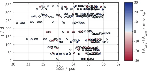
TA_calc = 738 + 43×SSS + 0.057×SSS² + 0.1205×t−3.46×10⁻⁴×t² (3.1) with TAcalc being the calculated alkalinity, SSS the sea surface salinity and t the day of year. The mean deviation of measured TAsam and TAcalc is 0.17µmol kg⁻¹ with a standard deviation ofσ = 12µmol kg⁻¹. Figure 3.6 shows the deviation as a function of salinity and the day of year. Using this estimated alkalinity and the measured seawater f CO2 values, the speciation within the carbonate system and the DIC concentration were calculated for each crossing with the inorganic carbon model CO2SYS (van Heuven et al., 2009) (CO2dissociation constants from Mehrbach et al. (1973), KSO⁻4 dissociation constants from Dickson and Millero (1987)). The small contributions of phosphate and

(47)

Figure 3.6: Deviation of sample alkalinity and alkalinity calculated from Equation 3.1 as a function of salinity and day of the year.

silicate to the alkalinity were neglected in this calculation because no underway measurements of these parameters were performed. Using maximum winter concentrations of phosphate (0.8µmol kg⁻¹) and silicate (6µmol kg⁻¹) the resulting maximum bias in TAcalc can be estimated to0.93µmol kg⁻¹. By comparing the calculated DIC (DICcalc) with measured DIC a good agreement of (3±7)µmol kg⁻¹ was found. For the salinity normalized DIC (nDIC) a alkalinity-salinity t was used to determine the intercept.

The salinity normalization was done using the Equation 3.2 to the mean salinity of each band, SSSmean (Friis et al., 2003). If the normalization was done towards a salinity of SSS_mean= 35psu, the resulting DIC is denoted as nDIC35.

nDIC = (DIC−683)×SSS_mean

SSS + 683 (3.2)

The CRDS isotope ratio measurements were calibrated and corrected for varying oxygen content with an instrument-specic equation. The δ¹³C(CO2) was then corrected to sea surface temperature by using the temperature dependent fractionation to DIC after Zhang et al. (1995):

(48)

δ¹³C (CO₂)_SST =δ¹³C (CO₂)_EQU−0.107 (T_EQU−T_SST) +

T_EQUf CO²⁻₃

EQU−T_SSTf CO²⁻₃

SST

(3.3)

with TEQUand TSST as the equilibrator and sea surface temperature andf CO²⁻₃

EQU

and f CO²⁻₃

SST the fraction of carbonate ions, calculated at the respective temperatures. The isotope ratio of DIC was calculated from the δ¹³C(CO2)EQU after Zhang et al. (1995) (please see Table 2.1). At the end, a moving average lter with a length of about 15 min was applied to the isotope ratio data in order to reduce the statistical noise. The chosen average time of 15 min is a compromise between improving the instrument precision by applying longer averaging times and still capturing observed gradients and natural variations that happen on a timescale shorter than the optimal averaging time of 150 min. The optimal averaging time for eld data was determined by comparing dierent averaging times during measurements of an intense bloom event.

The chosen averaging time did improve the data precision but did not mask features that were resolved with shorter averaging times and also observed in the f CO2 data.

The accuracy of the f CO2 measurements is estimated to be2µatmfor sea water. This sums up uncertainties stemming from the gas analyzer, the equilibration as well as the pressure and the temperature dierence between equilibrator and surface water. For the δ¹³C(CO2) measurements the accuracy is in the order of 0.15h while the conversion δ¹³C(DIC) introduces an additional uncertainty of about 0.15h.

3.3 Sample analysis

Discrete samples were taken during the crossings between 10^◦W and 55^◦W from the water supply line. The handling of the dierent samples is described below in more detail. The sampling locations are shown in Figure 3.4. The samples were taken every 3−7h. Assuming an average vessel speed of 18 kn this relates to a spatial resolution of 54−126sm between two samples.