Modeled Chl:C ratio and derived estimates of phytoplankton carbon biomass and its contribution to total particulate organic carbon in the global surface ocean

Modeled Chl:C ratio and derived estimates of phytoplankton carbon biomass and its contribution to total particulate organic carbon in the global surface ocean

Lionel Arteaga¹, Markus Pahlow², and Andreas Oschlies²

1Program in Atmospheric and Oceanic Sciences, Princeton University, Princeton, New Jersey,²GEOMAR Helmholtz Centre for Ocean Research Kiel, Kiel, Germany

Abstract

Chlorophyll (Chl) is a distinctive component of autotrophic organisms, often used as an indicator of phytoplankton biomass in the ocean. However, assessment of phytoplankton biomass from Chl relies on the accurate estimation of the Chl:carbon(C) ratio. Here we present global patterns of Chl:C ratios in the surface ocean obtained from a phytoplankton growth model that accounts for the optimal acclimation of phytoplankton to ambient nutrient, light, and temperature conditions. The model agrees largely with observed/expected global patterns of Chl:C. Combining our Chl:C estimates with satellite Chl and particulate organic carbon (POC), we infer phytoplankton C concentration in the surface ocean and its contribution to the total POC pool. Our results suggest that the portion of POC corresponding to living phytoplankton is higher in subtropical latitudes and less productive regions (∼30–70%) and decreases to

∼10–30% toward high latitudes and productive regions. An important caveat of our model is the lack of iron limiting effects on phytoplankton physiology. Comparison of our predicted phytoplankton biomass with an independent estimate of total POC reveals a positive correlation between nitrate concentrations and nonphotosynthetic POC in the surface ocean. This correlation disappears when a constant Chl:C is applied.

Our analysis is not constrained by assumptions of constant Chl:C or phytoplankton:POC ratio, providing a novel independent analysis of phytoplankton biomass in the surface ocean. These results highlight the importance of accounting for the variability in Chl:C and its application in distinguishing the autotrophic and heterotrophic components in the assemblage of the marine plankton ecosystem.

1. Introduction

Marine ecosystems contribute substantially to global biogeochemical fluxes by transporting photosyntheti- cally fixed organic carbon (C) and related nutrient elements from the sunlit surface layer to the deep ocean.

Photosynthesis by phytoplankton constitutes the principal supply route of organic carbon into the marine system. Understanding spatial and seasonal variations in phytoplankton biomass is a necessary requirement to assess the role of the ocean as a major regulator of the partitioning of carbon among atmosphere and ocean [Raven and Falkowski, 1999].

Phytoplankton carbon biomass is often inferred from chlorophyll measurements (Chl). However, Chl is a small and variable component of phytoplankton biomass and its ratio with respect to C (Chl:C) varies from<0.01 to>0.1 g Chl g C⁻¹in phytoplankton cultures [Geider, 1987, 1993]. Nutrient and light (co)limitation induces physiological changes in phytoplankton composition, which is reflected in the Chl:C ratio [Geider, 1987;

MacIntyre et al., 2000;Arteaga et al., 2014]. Inadequate representation of the physiological variability of the Chl:C ratio can result in poor estimates of marine productivity inferred from Chl [Siegel et al., 2001;Campbell et al., 2002;Behrenfeld et al., 2002]. Furthermore, deficient estimates of phytoplankton C biomass can lead to inaccurate descriptions of the trophic composition of the upper ocean, affecting the estimation of car- bon export [Emerson, 2014], metabolic rates [Ducklow and Doney, 2013] and how anthropogenically induced climate change affects marine ecosystems [Polovina et al., 2008].

In situ observations of phytoplankton Chl:C are scarce. Methods such as flow cytometry depend on informa- tion derived from fluorescence and scattering. These optically based estimates have associated uncertainties related to variable Chlafluorescence yields and a variable relationship between light scatter and carbon composition [Stramski and Reynolds, 1993]. More recently, optically based methods to estimate Chl:C and

RESEARCH ARTICLE

10.1002/2016GB005458

Key Points:

• Estimation of phytoplankton carbon biomass combining satellite- and model-based analyses

• Modeling of phytoplankton Chl:C ratio in the global surface ocean

• Assessment of phytoplankton biomass contribution to total particulate organic carbon in the surface ocean

Correspondence to:

L. Arteaga, laaq@princeton.edu

Citation:

Arteaga, L., M. Pahlow, and A. Oschlies (2016), Modeled Chl:C ratio and derived estimates of phytoplankton carbon biomass and its contribution to total par- ticulate organic carbon in the global surface ocean,Global Bio- geochem. Cycles,30, 1791–1810, doi:10.1002/2016GB005458.

Received 31 MAY 2016 Accepted 14 NOV 2016

Accepted article online 18 NOV 2016 Published online 17 DEC 2016

©2016. American Geophysical Union.

All Rights Reserved.

phytoplankton C biomass have been applied to data from satellite sensors and profiling floats, providing a more comprehensive description of the global surface ocean and the vertical variability of these biological quantities [Behrenfeld et al., 2005;Boss et al., 2015;Graff et al., 2015].

The diverse physiological effects of nutrient and light limitation on Chl:C can be represented in mechanistically founded phytoplankton models [Geider et al., 1998;Pahlow, 2005]. Cell quota models have the potential to represent variable phytoplankton elemental composition (e.g., C, nitrogen (N), phosphorus (P), and Chl), while optimality-based models provide the mechanistic foundation to describe physiological acclimation of phy- toplankton to a variable physicochemical environment [Smith et al., 2011]. The term optimality-based refers here to formulations describing the optimal allocation of resources (i.e., nutrients and energy) in order to max- imize cellular growth. Mechanistic models have been successfully employed to describe variations in the Chl:C ratio of phytoplankton cultures subject to nutrient and light stress [Geider et al., 1997;Pahlow, 2005;Pahlow and Oschlies, 2009;Pahlow et al., 2013]. However, to our knowledge, mechanistically-based global patterns of phytoplankton Chl:C ratio have not yet been inferred for the global surface ocean.

Here we estimate global surface Chl:C ratios employing a physiological phytoplankton growth model which maximizes growth by optimizing the net nutrient and energy balance of nutrient acquisition and light harvest- ing [Pahlow et al., 2013]. Model-based Chl:C estimates thus result from phytoplankton acclimation to nutrient and light availability. We force our model with monthly satellite-based temperature and light, model-based nitrate, and modelled mixed-layer depth information. When combined with independent satellite-based observations of surface Chl and particulate organic carbon (POC), we can then quantify global phytoplankton biomass and, for the first time, its contribution to total POC in the surface ocean.

2. Methods

We combine satellite-derived data with an optimality-based model of phytoplankton growth [Pahlow et al., 2013] (Figure 1) to obtain 1∘global monthly mixed layer phytoplankton Chl:C estimations for the period January 2005 to December 2010. The model defines the physiological roles of nitrogen and phosphorus via their association with specific functional cellular compartments [Sterner and Elser, 2002]. Growth is maxi- mized via optimal allocation of cellular N and energy among requirements for nutrient acquisition and light harvesting [Pahlow et al., 2013;Arteaga et al., 2014]. Thus, net C fixation is directly limited by cellular N, whereas phosphorus constrains nitrogen assimilation in the ribosomes and thereby limits nitrogen acquisi- tion. However, as phosphorus has been previously identified as a secondary limiting nutrient with respect to nitrogen in the global ocean surface layer (over time scales<1000 years) [Tyrrell, 1999;Arteaga et al., 2014], we restrict nutrient limitation in this study only to nitrogen and implicitly assume phosphate replete conditions throughout.

We use monthly satellite-based data to define temperature (sea surface temperature (SST)), light, and nitrate for the surface mixed layer [Arteaga et al., 2015]. Light is represented by the median mixed layer light level (I_g), which approximates the average light intensity experienced by phytoplankton cells in the surface mixed layer (I_g) [Behrenfeld et al., 2005],

I_g= 1

D⋅PAR⋅e^{−K490⋅MLD2} (1)

I_gdepends on the day-length fraction (D, the fraction of the day where light is available for photosynthe- sis), surface photosynthetically active radiation (PAR) (E m⁻²d⁻¹), the diffusive light attenuation coefficient estimated at 490 nm (K490) (m⁻¹) and mixed layer depth (MLD) (m).Dvaries as a function of the time of the year. Monthly SST, K490, and PAR inputs are obtained from the Moderate Resolution Imaging Spec- troradiometer (MODIS) (9 km, Level 3) (http://oceancolor.gsfc.nasa.gov). Monthly MLD is obtained from the Ocean Productivity site of Oregon State University (http://orca.science.oregonstate.edu/1080.by.2160.

monthly.hdf.mld.hycom.php). We employ always the most recent—and presumably improved—available MLD model output for our study period. For the period January–June 2005, monthly MLD is produced by an isothermal layer depth (ILD) model of the Thermal Ocean Prediction System (TOPS), which is a model of the Fleet Numerical Meteorology and Oceanography Center (FNMOC), Monterey, California, [Clancy and Martin, 1981;Clancy and Pollak, 1983;Clancy and Sadler, 1992] (ILD-TOPS). MLD for the period July 2005 to September 2008 is from a FNMOC high-resolution MLD criteria model (FNMOC-HIRES). Finally, monthly MLD between October 2008 and December 2010 is from the Hybrid Coordinate Ocean Model (HYCOM) [Bleck, 2002]. The use of different modeled MLD outputs is intended to cover the whole study period (2005–2010)

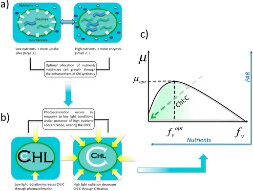
Figure 1.General concept of the optimality-based model. (a) Optimal allocation of nitrogen maximizes growth:

A greater nitrogen quota fraction (f_V) is allocated for nutrient acquisition when extracellular nutrient concentration is low (left). For higher nutrient concentrations more nitrogen is allocated for carbon fixation (right). Hence,f_Vincreases as the extracellular nutrient concentration drops. (b) The Chl:C ratio is the result of both photoacclimation and nitrogen allocation. With low light and sufficient nitrogen, Chl is synthesized to enhance light harvesting efficiency, resulting in an increased Chl:C ratio. High light conditions downregulate Chl production, decreasing Chl:C. (c) Net cell growth is maximized via optimal allocation of nitrogen resources. The Chl:C ratio is maximized by high nutrient-low light conditions and decreases as light levels increase and/or nutrient concentrations diminish.

with the most recent available model (i.e., MLD output is not available from HYCOM before October 2008 and FNMOC-HIRES before July 2005). Monthly global surface nitrate concentrations are taken from the data set produced byArteaga et al.[2015]. These global nitrate fields are obtained from multiple local linear regres- sions of satellite-derived SST, Chl, and model-based MLD. All input variables are regridded to a 1∘spatial resolution grid.

2.1. Determination of the Phytoplankton Chlorophyll-to-Carbon Ratio

The optimality-based model used in this study is thoroughly explained inPahlow et al.[2013]. Here we sum- marize briefly the regulation of the Chl:C ratio in the model (Figure 1). The Chl:C ratio is constrained by the effects of nutrient and light limitation on phytoplankton growth. Light (I_g) is used to estimate the degree of light saturation of the cellular light harvesting apparatus,S_I:

S_I=1−e

−^𝛼Iĝ𝜃 C VC

0 (2)

where𝛼is the Chl-specific light affinity,V₀^Cis the potential CO₂fixation rate, and̂𝜃^Cis the chlorophyll-to-carbon ratio of the chloroplast.S_Iand the fraction of internal resources allocated for cellular growth(1− ^QNs

Q^N −f_V) constrain the carbon fixation rate (V^C):

V^C=V₀^C (

1−Q^N_s Q^N−f_V

)

S_I (3)

wheref_Vis the fraction of cellular nitrogen allocated for nutrient acquisition,Q^Nis the nitrogen cell quota (N:C ratio) andQ^N_s represents cellular nitrogen bound in structural protein. Nutrient and light limited phytoplank- ton growth is described as the difference between carbon fixation (V^C) and respiration (R):

𝜇=V^C−R. (4)

Chlorophyll synthesis is driven by the balance of CO₂fixation and the cost of photosynthesis incurred within the chloroplast. As discussed inArteaga et al.[2014], the Chl:C ratio is regulated to maximize the energy avail- able for carbon and nutrient assimilation. The first step to calculate the Chl:C ratio is the determination of the Chl:C ratio of the chloroplasts:

̂𝜃^C= 1 𝜁^Chl + V₀^C

𝛼I_g {

1−W₀ [(

1+ R^Chl_m DV₀^C

) e

𝛼Ig VC

0𝜁Chl+1]}

ifI_g>I_g0

̂𝜃^C=0 if I_g≤I_g0

(5)

where𝜁^Chlis the cost of photosynthesis,R^Chl_m is the cost of Chl maintenance,

I_g0= 𝜁^ChlR^Chl_m

D𝛼 (6)

is the threshold irradiance for chlorophyll synthesis, andW₀is the 0 branch of the Lambert-W function, defined by W(x)e^W(x)=x[Barry et al., 2000].

The Chl:C ratio of the entire cell is then obtained as a direct result of N and light limitation, represented byQ^N and̂𝜃^C, respectively:

Chl:C= ̂𝜃^C (

1−Q^N_s Q^N−f_v

)

. (7)

2.1.1. Temperature Dependence

Since the original model [Pahlow et al., 2013] does not include temperature, we introduce a temperature dependence (TEMP, degree Celsius) [Eppley, 1972] of the maximum rate parameters, in the same manner as inArteaga et al.[2014]:

V₀^C=V₀^N=V₀^P=1.4∗1.066^TEMP (8) 2.2. Spatial Parametrization of Phytoplankton Nutrient and Light Affinity

Oceanic surface observations of Chl:C and phytoplankton C are sparse. Overall, an inverse global correlation between Chl:C and light is expected due to phytoplankton photoacclimation [Geider, 1987]. Some of these global patterns are captured by the optically derived Chl:C ratio estimated byBehrenfeld et al.[2005]. The novel feature inBehrenfeld et al.[2005] is the estimation of phytoplankton carbon via the backscattering coef- ficient (bbp) at 440 nm. Chl concentrations in that study were inferred from the ample and standardly used water-leaving radiance data set provided by the Sea-viewing Wide Field-of-view Sensor. As the optically based algorithm developed byBehrenfeld et al.[2005] currently provides, to the best of our knowledge, the only reference for global estimates of Chl:C on a relatively high temporal resolution (i.e., monthly), we aimed to produce model-based outputs of Chl:C that are in the same range as what is predicted by the algorithm of Behrenfeld et al.[2005].

In order to represent different phytoplankton communities adapted to varying nutrient and light limitation regimes, we introduce a simple parametrization for the phytoplankton Chl-specific light affinity (𝛼) and nutri- ent affinity (A₀) in the optimality-based model. The assignment of varying𝛼 andA₀is implemented as a two-step procedure: First, an initial parameter set (Table 1) is applied with mean values obtained for differ- ent phytoplankton species [Pahlow et al., 2013]. As mentioned above, the optimality-based model predicts the biomass-normalized nitrogen cell quota (phytoplankton N:C ratio,Q^N) and the estimated degree of light saturation of the cellular light harvesting apparatus (S_I). We useQ^NandS_Ito infer nitrogen and light limita- tion, respectively [Arteaga et al., 2014]. Nitrogen limitation (L_N) is defined as the relative difference between Q^Nand the phytoplankton subsistence quota (Q^N₀). Light limitation (L_I) is defined as one minus the degree of light saturation:

L_N=1−Q^N−Q^N₀ Q^N =Q^N₀

Q^N (9)

L_I=1−S_I (10)

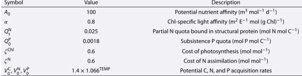
Table 1.Model Parameters Description and Values Used in the Standard Run

Symbol Value Description

A₀ 100 Potential nutrient affinity (m³mol⁻¹d⁻¹)

𝛼 0.8 Chl-specific light affinity (m²E⁻¹mol (g Chl)⁻¹)

Q^N_s 0.025 Partial N quota bound in structural protein (mol N mol C⁻¹)

Q^P₀ 0.0018 Subsistence P quota (mol P mol C⁻¹)

𝜁^Chl 0.6 Cost of photosynthesis (mol mol⁻¹)

𝜁^N 0.6 Cost of N assimilation (mol mol⁻¹)

V₀^C,V₀^N,V^P₀ 1.4×1.066^TEMP Potential C, N, and P acquisition rates

whereL_N = 0andL_l = 0(dimensionless) indicate no limitation andL_N = 1andL_l = 1indicate strong limitation. The resulting patterns ofL_NandL_Iare thus assumed to represent the global distribution of nitrogen and light limiting regions for an average phytoplankton cell [Ward et al., 2012;Arteaga et al., 2014].

In the second step, we employL_IandL_Nobtained during the first step to assign varying𝛼andA₀and thereby to represent multiple phytoplankton communities adapted to different light and nitrogen limitation regimes across the global ocean. We apply a simple linear formulation, where𝛼andA₀are directly proportional to monthly mean light and nitrogen limitation, respectively:

𝛼=a_𝛼L_I+b_𝛼 (11)

A₀=a_AL_N+b_A. (12)

After testing different slopesaand offsetsb, we achieve a reasonable agreement with global optically derived Chl:C ratios [Behrenfeld et al., 2005] fora_𝛼 = 1(m²E⁻¹mol (g Chl)⁻¹),a_A = 100(m³mol⁻¹d⁻¹),b_𝛼 = 0.3 (m²E⁻¹mol (g Chl)⁻¹), andb_A=40(m³mol⁻¹d⁻¹). The form of equations (11) and (12) was chosen because it represents the simplest relation between light and nutrient limitation and respective affinities and is not aimed to describe a particular mechanism. Nevertheless, adaptation to nutrient or light limited conditions could be expected to result in positive correlations between the affinities and their respective limitation indices. Thus, equations (11) and (12) could be viewed as a phenomenological representation of the effects of evolution of specific traits, such as cell size (nutrient affinity) or pigment composition (light affinity) in local phytoplankton communities. The resulting distributions of𝛼andA₀employing the coefficients above (aandb) are within the ranges of different phytoplankton species [Pahlow et al., 2013]. A sensitivity analysis shows that alterations of 10% for different combinations of these coefficients do not substantially alter the obtained patterns of modeled Chl:C (see section 4 below). The resulting distribution of phytoplankton species produces a general latitudinal pattern composed of phytoplankton with high𝛼and lowA₀in high latitudes and vice versa in tropical regions (Figures 2a and 2b). The distribution of nutrient and light limitation areas derived from the spatial parametrization of𝛼andA₀does not deviate from that obtained in the first step (Figures 2c and 2d).

2.3. Estimation of Phytoplankton Carbon

We estimate global living phytoplankton carbon (phytoC) in the surface ocean from our predicted Chl:C ratio and observations of surface Chl from the MODIS sensor (Chl_MODIS, mg C m⁻³)

phytoC= (Chl:C)⁻¹_m ⋅Chl_MODIS (13)

where Chl:C_mis the predicted (model-derived) Chl:C ratio and phyto C is obtained in mg C m⁻³. Satellite-based observations of Chl provide valuable information on the relative patterns of phytoplankton biomass in the global surface ocean. The incorporation of a physiologically derived Chl:C ratio allows a mechanistically founded (with exception of equations (11) and (12)) description of the distribution of phytoplankton carbon biomass at the surface of the global ocean.

Since the light level driving photoacclimation is given by I_g, our estimated Chl:C ratio represents an average for the surface mixed layer. Our phytoC estimates also depend on satellite-derived Chl. Satellite-borne ocean color instruments estimate the upwelling spectral radiant flux at the sea surface by measuring

Figure 2.Global distribution of (a) nutrient (A₀) and (b) light affinities (_𝛼) as functions of nutrient and light limitation, respectively. Areas of nutrient

(i.e., nitrogen) limitation are defined by the relative difference betweenQ^NandQ^N₀, while light limitation regions are defined a by one minus the degree of light saturation (1−S_I).Q^NandS_Iare inferred for the global ocean by the model ofPahlow et al.[2013]. Phytoplankton adapted to low nutrient and high light conditions are characterized by highA₀and low_𝛼, and vice versa for phytoplankton adapted to high nutrient-low light conditions. Difference in the global distribution of (c) nitrogen limitation (L_N) and (d) light limitation (L_I) indices, between the second (output) run with variable_𝛼andA₀, and the initial (standard) run with constant_𝛼andA₀(i.e., second run-first run). L_Nand L_Ican vary between 0 and 1.

the spectral radiant flux emanating upward from the top of the atmosphere, accounting for atmospheric corrections [Werdell and Bailey, 2005]. Surface Chl from remote sensors is estimated measuring the small portion of incident radiation not absorbed by the ocean and its constituents [Longhurst, 2007], using empir- ical algorithms based on large in situ data sets [Werdell and Bailey, 2005]. Even in the clearest waters the depth from which information can be retrieved via remote sensing rarely exceeds 25 m [Kemp and Villareal, 2013]. Thus, as long as the mixed layer is deeper than the depth range seen by the satel- lite and as cells within the mixed layer are mixed faster than they can adapt to light gradients within the mixed layer [Moore et al., 2003], remotely sensed information will be representative of that of the mixed layer.

We use independent satellite-based estimates of total surface POC [Dufor˙et-Gaurier et al., 2010] to assess the relative contribution of living phytoplankton carbon to the total POC pool at the surface (phytoC_rel).

phytoC_rel= PhytoC

POC_sat. (14)

Satellite surface POC estimates (POC_sat) are obtained as described inDufor˙et-Gaurier et al.[2010] by the aver- age of two methods: based on an empirical power law between surface POC and the blue-to-green ratio of the remote sensing reflectance [Stramski et al., 2008] and based on deriving surface POC from a remotely sensed inherent optical property [Loisel et al., 2002].

In the following sections we start by describing the general patterns of estimated Chl:C and a comparison against in situ estimates (sections 3.1 and 3.2). We then describe our estimates of phytoplankton C biomass and discuss the importance of accounting for the variability in the Chl:C ratio to assess the contribution of living phytoplankton to total POC (sections 3.3 and 3.4). At the end of section 3 we discuss the caveats and discrepancies between our model-based estimate of Chl:C and that derived from a remote sensing optical algorithm (section 3.5). A series of sensitivity analyses of our modeled Chl:C is presented in section 4. We end by highlighting the main results of this study in our conclusions.

Figure 3.Global patterns of phytoplankton Chl:C ratio obtained with the (a and b) optimality-based physiological model [Pahlow et al., 2013] and the (c and d) optically based method ofBehrenfeld et al.[2005]. Figures 3a and 3c correspond to mean monthly values for the boreal summer (April–September), whereas Figures 3b and 3d represent mean values for the austral summer. White regions indicate areas with no data.

3. Results and Discussion

3.1. Global Chl:C Patterns

Our estimated surface Chl:C ratios (Figures 3a and 3b) vary seasonally and geographically from<0.01 to 0.05 g Chl g C⁻¹. Lowest Chl:C values are predicted for the tropical and subtropical ocean, with the excep- tion of the equatorial Pacific. Highest model-based Chl:C ratios are obtained during winter in high latitudes polarward of 40∘in the Southern Ocean and northern Atlantic and Pacific Oceans. The seasonality of our model-based Chl:C is driven by the availability of nutrients and light. Phytoplankton physiology adapts to low light levels by increasing the synthesis of Chl [Geider, 1987]. However, photoacclimation occurs more effectively during high nutrient conditions, as nitrogen is a key enzymatic compound of the photochemical machinery of the cell [Kolber et al., 1988]. As a result, high Chl:C is predicted during high nutrient-low light conditions and vice versa.

3.2. Comparison Against In Situ Estimates of Chl:C

The ability of the optimality-based model to reproduce Chl:C in phytoplankton experiments was validated in Pahlow et al.[2013] for light and nutrient limited laboratory cultures [Laws and Bannister, 1980;Terry et al., 1985;

Healey, 1985;Rhee, 1974]. In situ observations are scarce, and the most comprehensive global picture for phy- toplankton Chl:C is provided byBehrenfeld et al.[2005], although these are empirical model-based results and

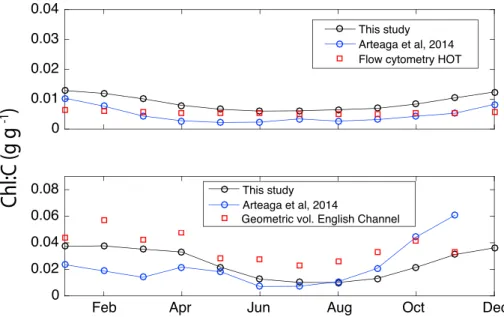
Figure 4.Monthly patterns of phytoplankton Chl:C ratio in the (a) Hawaii Ocean Time series (HOT) and (b) English Channel. Red squares are flow cytometry data for HOT [Winn et al., 1995] scaled to Chl:C [Westberry et al., 2008] and combined cell volume and high-performance liquid chromatography (HPLC) measurements in the English Channel [Llewellyn et al., 2005]. Black circles connected with lines are model-based results for this study. Blue circles connected with lines are model results fromArteaga et al.[2014].

not in situ observations.Arteaga et al.[2014] compared Chl:C estimates obtained using the optimality-based model ofPahlow et al.[2013] against fluorescence measurements at the Hawaii Ocean Time series (HOT) [Winn et al., 1995], scaled to Chl:C [Westberry et al., 2008] and combined cell volume and high-performance liquid chromatography (HPLC) measurements in the English Channel [Llewellyn et al., 2005]. Here we employ the same observations to compare our model-based outputs. The only difference between our model-based results and those ofArteaga et al.[2014] is the geographical parametrization of the light and nutrient affinities applied in this study.

Our mean monthly Chl:C outputs for 2005–2010 reproduce the seasonal evolution of the observations at both sites reasonably well (Figure 4). Model outputs for this study (correlation coefficient (r) = 0.85, root-mean-square error (RMSE) = 0.003 g Chl g C⁻¹) slightly overestimate Chl:C observations at HOT, whereas previous estimates fromArteaga et al.[2014] (r= 0.81, RMSE = 7.6×10⁻⁴g Chl g C⁻¹) showed a slight under- estimation. Inferred model-based Chl:C in this study for the English Channel (r= 0.84, RMSE = 0.013) is higher and overall closer to observations than Chl:C inferred inArteaga et al.[2014] (r= 0.2, RMSE = 0.014 g Chl g C⁻¹).

Overall, the spatial parametrization of light and nutrient affinities applied in this study increases Chl:C ratio estimates, bringing them closer to observations at HOT and the English Channel compared to the estimates fromArteaga et al.[2014].

3.3. Phytoplankton C in the Global Surface Ocean

Phytoplankton C (phytoC) in the global surface ocean is computed from satellite-inferred surface Chl from MODIS and our model-based Chl:C ratio estimates (i.e., phytoC=Chl_MODIS⋅(Chl:C)⁻¹_m) (Figures 5a and 5b). High phytoC concentrations are predicted during summer months for each hemisphere. During the northern sum- mer (April–September), high phytoC concentrations are found in high northern latitudes, particularly in the Atlantic Ocean. During austral summer, phytoC concentrations are high in the high southern latitudes, partic- ularly near New Zealand and the Atlantic coast of southern South America. This seasonal pattern is the result of differences in Chl concentration and the Chl:C ratio between the two hemispheres, with Chl:C being higher in the winter hemisphere due to photoacclimation by phytoplankton cells [Geider, 1987;MacIntyre et al., 2000].

Estimated phytoC is highest in coastal regions, where it reaches concentrations of about 30 mg C m⁻³. The Caribbean and Indian Ocean also show high phytoC concentrations throughout the year. Predicted phytoC in the central Atlantic varies from<10 mg C m⁻³to∼15 mg C m⁻³, consistent with observations in this region [Wang et al., 2013]. Our physiological model employed to estimate Chl:C, and hence phytoC, does not account for the physiological effects of iron limitation on phytoplankton. However, iron limitation is implicitly included

Figure 5.(a and b) Surface phytoplankton carbon concentration inferred from the optimality-based model and MODIS-Chl. (c and d) Surface POC in the global ocean, estimated as inDufor˙et-Gaurier et al.[2010]. (e and f ) Relative phytoplankton carbon contribution to total surface POC in the global ocean. (g and h) Relative phytoplankton carbon contribution of total POC (same as Figures 5e and 5f but showing only low values, up to 0.3). Figures 5a, 5c, 5e, and 5g are the mean of northern summer months (April–September) for the period 2005–2010. Figures 5b, 5d, 5f, and 5h) are the northern winter months mean

(October–March).

to some degree in the estimation of phytoC by using Chl satellite observations (this is not the case for our Chl:C estimates, which do not depend on satellite Chl information). Iron deprivation should reduce phytoplankton growth rates and Chl synthesis, and hence decrease Chl:C [Geider and LaRoche, 1994]. Accounting for iron dynamics in our model-based analysis should thus result in higher phytoC concentrations in the Southern Ocean, where iron limitation is particularly important [Martin et al., 1990;Boyd et al., 2007]. Higher estimates of phytoC expected from our model-based analysis are due to the effect of iron limitation reducing Chl:C [Sunda and Huntsman, 1997] and should not be confused with an enhancement of growth rates under iron limitation.

3.4. Living Phytoplankton Contribution to POC 3.4.1. Spatial Patterns

Combining our phytoC estimates with satellite-derived surface POC concentrations (Figures 5c and 5d) allows us to infer the contribution of living phytoplankton to the total particulate organic carbon biomass in the global surface ocean (phytoC_rel) (Figures 5e–5h). This relative contribution, phytoC_rel, follows a similar sea- sonal trend between hemispheres as phytoC and POC. Nevertheless, while phytoC and POC show similar regional patterns generally decreasing toward the subtropical gyres, their ratio (i.e., the contribution of living phytoplankton to surface POC) displays an inverse latitudinal pattern with respect to total surface POC con- centration and phytoC. According to our estimates, living phytoplankton comprises between 30 and 70% of total surface POC in most of the low-latitude ocean, between 40∘north and 40∘south (Figures 5e and 5f ).

However, its share of the total surface POC decreases toward the poles in both hemispheres, where phyto- plankton C constitutes between 10 and 30% of total surface POC (Figures 5g and 5h). Low phytoC_relis also diagnosed in the productive region of the equatorial Pacific. The most pronounced seasonal variation in rela- tive phytoplankton biomass occurs in the Pacific Ocean. Surface phytoplankton C contribution to POC is high in the North Pacific during boreal summer months (April–September) and south of the equator during boreal winter months (October–March). The contribution of phytoC in the Southern Ocean is fairly constant dur- ing both summer and winter. According to our analysis, the Southern Ocean also has the lowest contribution of phytoC (≈10%) throughout the global surface ocean. However, this contribution might be higher if iron limitation was considered, due to the effects of iron deprivation on the Chl:C ratio (see section 3.5).

We compare the latitudinal gradient of our phytoC estimates with in situ POC observations of the surface ocean (top 10 m) obtained fromMartiny et al.[2014] and satellite-inferred surface POC (Figure 6a). Latitu- dinal patterns are obtained as zonal horizontal averages for each latitudinal band where observations and model outputs for a 6 year climatological mean (2005–2010) are available. Surface POC (in situ and satellite inferred) and estimated phytoC are both larger at high latitudes and decrease toward the equator. Similar to Figures 5e–5h, surface POC observations [Martiny et al., 2014] decline more rapidly toward tropical regions than phytoC, implying that the phytoC contribution to total POC is larger in low latitudes. The average latitudi- nal satellite-derived surface POC follows a similar trend as the in situ POC observations for the surface ocean, providing confidence in the global patterns of living phytoplankton C contribution to total POC in the surface shown in Figures 5e–5h. Our modeled phytoC does not show a strong latitudinal increase toward southern latitudes, possibly as a result of neglecting iron limitation.

3.4.2. Relationship Between POC Partitioning and Surface Nutrient Concentration

Our global maps show a relative partitioning of particulate carbon between photosynthetic organisms and other particles in the surface ocean. The partitioning of dissolved organic carbon or inorganic carbon com- pounds is not assessed by our study. The remaining portion of POC (1-phytoC_rel) corresponds to other living forms of carbon (i.e., bacteria and zooplankton) as well as detrital organic carbon compounds. The pattern shown in Figure 6a indicates a positive correlation between nutrient concentration and the contribution of nonphytoplankton particles to POC in the global surface ocean. This correlation is confirmed when we plot the zonal mean contribution of nonphytoplankton particles (1-phytoC_rel=1−^PhytoC

POC_sat) against the zonal mean nitrate concentration for each latitudinal band. Estimations of 1-phytoC_relderived from our global analysis of variable Chl:C ratio indicate a saturating increase of the nonphytoplankton contribution to the total POC pool as nitrate concentrations rise (Figure 6b). We analyze the same relationship employing the phytoplankton C biomass derived from a remotely sensed backscattering signal (C_phyto) [Behrenfeld et al., 2005] (Figure 6c).

A similar pattern is found when the optically derived C_phyto is used. This result is somewhat unexpected, as the empirical relation used to estimate phytoplankton C from particle backscattering assumes a stable nonalgal (heterotrophic and detrital) background component, and its scalar coefficient was chosen so that retrieved C_phyto:POC ratios were∼0.3, which is the mean value of the limited field measurements analyzed

Figure 6.(a) Latitudinal patterns in modeled surface phytoplankton carbon (phytoC) (blue line and circles),

satellite-inferred surface POC (red squares), and POC surface observations (top 10 m, black asterisks) fromMartiny et al.

[2014]. Contribution of nonphytoplankton carbon to total POC in the surface ocean (1-phytoC_rel) versus surface nitrate concentration: Phytoplankton carbon was inferred using (b) the optimality-based model [Pahlow et al., 2013], (c) the optically (backscattering) based algorithm [Behrenfeld et al., 2005], and (d) a constant global ratio of 0.01 g Chl g C⁻¹. All latitudinal patterns are obtained as zonal averages for each latitudinal band where observations and modeled outputs are available.

inBehrenfeld et al.[2005]. Given this constraint, we expected that 1-phytoC_relas inferred from the optically derived C_phyto, to be∼0.7 for all nitrate concentrations. Overall, 1-phytoC_relcomputed from C_phytois∼0.7 for nitrate concentrations>3μmol l⁻¹, but lower values are obtained for nitrate concentrations<3μmol l⁻¹. The connection between nitrate and 1-phytoC_relis not evident when phytoplankton C is computed employing a constant Chl:C ratio (0.01 g Chl g C⁻¹) for the global ocean (i.e., when the variability in the Chl:C ratio is ignored) (Figure 6d). In fact, for zonal mean estimates obtained for the Northern Hemisphere, the relationship between 1-phytoC_reland nitrate is negative. This is likely due to a positive correlation between satellite-based Chl and surface nitrate, which could be misconceived as a positive relation between nutrients and phytoplankton biomass if the physiological acclimation of the Chl:C ratio is ignored.

While our analysis does not allow us to discern between the contributions of zooplankton, other heterotrophs, or detritus to 1-phytoC_rel, it is reasonable to expect that high values of 1-phytoC_relare at least partially due to an increase in the zooplankton share of total POC associated with regions of high nitrate concentration.

This pattern is consistent with the view that in general, marine ecosystems are composed of grazer con- trolled phytoplankton populations in nutrient-limited systems [Price et al., 1994;Talmy et al., 2016]. Idealized population models with size-specific grazing relationships suggest that top-down controls determine the phytoplankton biomass of a given size class, whereas bottom-up nutrient limitation ultimately regulates the total biomass in the system [Armstrong, 1994;Thingstad and Sakshaug, 1990]. Our results coincide with predic- tions from ecological models suggesting that the ratio of zooplankton:phytoplankton increases with higher

nutrient and phytoplankton biomass, as a larger fraction of the community is brought under top-down control [Ward et al., 2012, 2014].

Our zonally averaged plot of 1-phytoC_relagainst nitrate based on the optimal growth model Chl:C estimates (Figure 6b) shows clearly distinct relations for the Southern and Northern Hemispheres. Model outputs for the Southern Hemisphere suggest a higher fraction of nonphytoplankton material in the POC pool for the same nitrate concentration compared to the Northern Hemisphere. A similar interhemispheric difference is also noticeable when a fixed Chl:C ratio is used to estimate phytoC (Figure 6d). An inverse but less pronounced dis- tinction is shown when the optically based C_phytois used to infer 1-phytoC_rel(Figure 6c). It is unclear whether this interhemispheric pattern is related to distinct ecological processes between hemispheres or induced by differences in the model-based estimations of Chl:C and phytoC (optical algorithms versus mechanistic for- mulations of phytoplankton physiology), as the difference between hemispheres is not present in the same manner in all three analyses (Figures 6b–6d). We do not find similar distinctions between ocean basins. Our optimality-based Chl:C estimates predict a decreasing fraction of phytoplankton C to total POC (i.e., higher 1-phytoC_rel) toward high nitrate concentrations in the Southern Hemisphere. Iron limitation could explain this inferred low share of POC assigned to living phytoplankton in regions of the Southern Hemisphere with higher nitrate concentrations (>10μmol l⁻¹), characteristic of the Southern Ocean [Moore et al., 2013, 2001;Boyd et al., 2010]. As mentioned above, iron is not part of our optimality-based model, but partial effects of iron lim- itation are implicitly accounted for in our estimates of phytoC by the use of satellite-based Chl observations to compute phytoC. Low phytoplankton contribution to POC is also shown for lower nitrate concentra- tions (<10μmol l⁻¹) in the Southern Hemisphere, compared to the Northern Hemisphere (Figure 6b). Both bottom-up and top-down processes, such as limitation by other nutrients (e.g., silicon limitation, [Sarmiento et al., 2004a]), could be responsible for causing the variation in the relative composition of the POC pool.

3.5. Differences and Considerations of the Optical and Model-Based Estimates of Chl:C Ratio and Phytoplankton C Biomass

The optimality-based Chl:C patterns presented in this work are, together with the satellite-based estimates of Behrenfeld et al.[2005], the only two studies assessing the global distribution of Chl:C ratios in the surface ocean that we are aware of. Our model-based Chl:C global and seasonal patterns are similar to those predicted by the optically based algorithm ofBehrenfeld et al.[2005] (monthly estimates of optically derived phytoplank- ton C (C_phyto) for 2005–2010 are obtained from http://orca.science.oregonstate.edu/1080.by.2160.monthly.

hdf.carbon2.m.php) (Figures 3c and 3d). Optically derived Chl:C is higher in high latitudes (particularly during winter), the equatorial Pacific, and lower in the oligotrophic gyres in the Atlantic and Pacific Oceans. The most obvious discrepancies between our model-based and the optically based Chl:C estimates are the high values inferred by the optical algorithm along continental margins and the tropical Atlantic and Indian Oceans, as well as the high values predicted by the optimality-based model in the Southern Ocean (Figure 7a). The optically inferred Chl:C shows maximum values close to the continental margins (≥0.05 g Chl g C⁻¹). As the satellite-based Chl:C product is essentially a Chl:backscattering ratio that depends directly on Chl estimated from a satellite sensor (i.e., MODIS), high values in this ratio may be associated with known errors in the retrieval of Chl from satellites due to the interference of colored dissolved organic matter (CDOM) and detritus [Siegel et al., 2005;Morel and Gentili, 2009;Loisel et al., 2010]. In the same manner, errors associated to the accu- rate retrieval of Chl concentration from ocean color can affect our model-based estimates of phytoplankton C biomass, which depend on MODIS Chl observations (equation (13)).

An important source of discrepancy between both methods is the assumption stated inBehrenfeld et al., 2005 [2005, section 3.1] that“...the particle population contributing to bbp is comprised of a stable non-algal back- ground component and a second component that includes phytoplankton and other particles that covary with phytoplankton.”According to our interpretation, this implies that the phytoplankton C contribution to POC is roughly constant in the global ocean. This contribution of∼30% is aimed to represent a range of phy- toplankton C:POC ratios that vary from 19% to 49% for different oligotrophic and eutrophic regions of the global ocean [seeBehrenfeld et al., 2005, and references therein, sections 2.3 and 3.1]. Our model-based Chl:C ratio estimates make no a priori assumption about phytoplankton C:POC and therefore provide an inde- pendent estimate of this ratio in the surface ocean (i.e., phytoC_rel, Figures 5e–5h). Comparing the regional differences in estimated Chl:C ratio from the optical method ofBehrenfeld et al.[2005] and the model-based results obtained in this work (Figure 7), we find that the highest degree of agreement between these two independent estimates occurs in regions where our estimate of phytoC_relis around∼30% (i.e., the range of

Figure 7.(a) Map of global differences in estimated surface Chl:C ratio between the optical method ofBehrenfeld et al.[2005] and the model-based results obtained in this study. (b) Scatterplot of the relative phytoplankton C biomass contribution to total POC in the surface ocean (phytoC_rel) and differences in predicted Chl:C ratio (optical-model based results) for the Atlantic, (c) Pacific, and (d) Indian Oceans. Black dashed line in the scatterplots shows perfect agreement of predicted Chl:C by both optical and model-based estimates. Red dashed line shows the location of data points where phytoC_relis=0.3, which is the portion of phytoplankton to total POC aimed at by the linear model ofBehrenfeld et al.[2005] to estimate phytoplankton C from surface ocean backscattering.

phytoplankton C: POC ratios aimed at by the linear model ofBehrenfeld et al.[2005]). Regions of the Atlantic, Pacific, and Indian Oceans where the optical method predicts higher Chl:C than our model analysis correlate well with regions where our estimate of phytoC_relis>30%, while regions where the optical method predicts lower Chl:C than our model-based results correspond to regions where our estimate of phytoC_relis<30%.

While our model-based estimates cannot be interpreted as true observations of Chl:C, these results suggest that the optically based algorithm may be inaccurate in regions where phytoC_reldeviates substantially from 30%, and hence, this backscattering-dependent relationship should be employed with caution.

Differences between these two estimates in regions where the predicted model-based Chl:C is larger than the optically derived Chl:C (i.e., Southern Ocean and tropical Pacific) are likely not only associated to inaccuracies in the optical estimate caused by deviations of the phytoplankton C:POC ratio from 0.3. High estimates of Chl:C ratio predicted by the optimal growth model with respect to the optical algorithm might be an overestimation of the model-based results due to the lack of iron limitation in the model. Iron deprivation should suppress nitrogen uptake and reduce photosynthetic electron transfer efficiency [Geider and LaRoche, 1994]. Thus, the inclusion of iron dynamics in the model is expected to result in a reduction of the predicted Chl:C ratio in iron limited areas, such as the Southern Ocean [Sunda and Huntsman, 1997;Martin et al., 1990].

As mentioned above, our range of predicted Chl:C in the global ocean varies from<0.01 to 0.05 g Chl g C⁻¹, consistent with Chl:C obtained in phytoplankton cultures [Laws and Bannister, 1980;Geider, 1993]. Our model-based results predict Chl:C<0.01 in large areas of the tropical and subtropical ocean. As a conse- quence of the large oceanic area covered by these regions, our mean globally modeled Chl:C ratio is∼0.01 (g g⁻¹), which is the median value found in laboratory data compiled byBehrenfeld et al.[2002] for light levels between 0.7 and 1.4 moles photons m⁻²h⁻¹. We evaluate the regional effects of estimating phytoplankton C

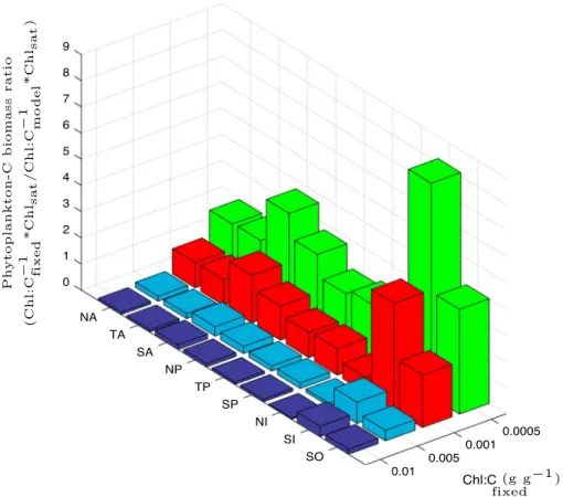
Figure 8.Ratio of predicted phytoplankton carbon biomass obtained as the product of satellite-derived Chl (Chl_sat) and a fixed Chl:C ratio (Chl:C⁻¹_fixed) and Chl_satcombined with our model-based Chl:C ratio (Chl:C⁻¹_model) (i.e., Chl:C⁻¹_fixed*Chl_sat/ Chl:C⁻¹_model*Chl_sat= Chl:C_model∕Chl:C_fixed), for different regions of the global ocean: North Atlantic (NA) (20^∘N–90^∘N, 100^∘W–0^∘W), Tropical Atlantic (TA) (20^∘S–20^∘N, 70^∘W–0^∘W), South Atlantic (SA) (50^∘S–20^∘S, 70^∘W–20^∘E), North Pacific (NP) (20^∘N–90^∘N, 110^∘E–100^∘W), Tropical Pacific (TP) (20^∘S–20^∘N, 110^∘E–90^∘W), South Pacific (SP) (50^∘S–20^∘S, 120^∘E–70^∘W), North Indian (NI) (10^∘S–20^∘N, 40^∘E–110^∘E), South Indian (SI) (50^∘S–10^∘S, 40^∘E–110^∘E), and Southern Oceans (SO) (0^∘S–50^∘S).

biomass from satellite Chl employing different globally constant (fixed) Chl:C ratios, in comparison with our model-based Chl:C (i.e., Chl:C⁻¹_fixed*Chl_sat/Chl:C⁻¹_model*Chl_sat) (Figure 8). Overall, the closest match in pre- dicted phytoplankton C biomass from fixed and model-based Chl:C (employing the same satellite Chl information) occurs when Chl:C is∼0.001 (g g⁻¹). This relatively low fixed Chl:C needed to match our predicted phytoplankton carbon biomass is a consequence of the large regions of the global ocean with predicted Chl:C ratios<0.01 (g g⁻¹). Compared with our estimates, using a globally fixed Chl:C to infer phytoplankton biomass can have diverse effects in different regions of the global ocean, which can result in a overestimation of 2–8 times in phytoplankton C concentration (or underestimation depending on the fixed Chl:C employed to infer phytoplankton C). This analysis highlights the importance of accounting for regional differences in Chl:C in order to estimate phytoplankton carbon biomass.

4. Sensitivity Analyses

4.1. General Parameter Sensitivity

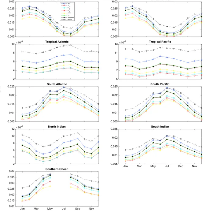
We conducted several sensitivity analyses in order to evaluate the effect of each model parameter presented in Table 1 on the estimated phytoplankton Chl:C ratios. We performed six additional simulations for the year 2005, increasing each of the six non-temperature-dependent parameters of the model by 50%. The results of these calculations for different ocean basins are presented in Figure 9. Compared against our standard con- figuration, our model-based Chl:C is most sensitive to changes in phytoplankton nutrient affinity (A₀) and the Chl-specific light absorption coefficient (𝛼). A greaterA₀results in a reduction of the nitrogen limitation experienced by phytoplankton, enlarging the internal pool of the enzymatic material available for the photo- chemical machinery, which results in a higher Chl:C ratio. Conversely, a larger𝛼results in a more efficient use of light, reducing Chl:C.

Figure 9.Sensitivity experiments (colored solid lines and symbols) based on monthly results for 2005. For each experiment, all non-temperature-dependent model parameters are kept globally constant as in Table 1, except for one parameter whose value was incremented by 50% with respect to Table 1. The solid back lines show the “standard” configuration with globally constant values for non-temperature-dependent parameters. The black dashed lines show the

“output” run, which includes the spatial parametrization ofA₀and_𝛼. Missing data in the Southern Ocean are due to the lack of satellite information during winter months. Geographical regional bundaries: North Atlantic (20^∘N–90^∘N, 100^∘W–0^∘W), Tropical Atlantic (20^∘S–20^∘N, 70^∘W–0^∘W), South Atlantic (50^∘S–20^∘S, 70^∘W–20^∘E), North Pacific (20^∘N–90^∘N, 110^∘E–100^∘W), Tropical Pacific (20^∘S–20^∘N, 110^∘E–90^∘W), South Pacific (50^∘S–20^∘S, 120^∘E–70^∘W), North Indian (10^∘S–20^∘N, 40^∘E–110^∘E), South Indian (50^∘S–10^∘S, 40^∘E–110^∘E), and Southern Oceans (0^∘S–50^∘S).

Increasing the cost of photosynthesis (𝜁^Chl), the cost of N assimilation (𝜁^N), or the subsistence nitrogen and phosphorus cell quotas (Q^N_s,Q^P₀) has more moderate effects on Chl:C in comparison toA₀and𝛼. Both𝜁^Chland 𝜁^Nincrease the cost of Chl synthesis; thus, higher values lead to lower Chl:C ratios. A 50% increase inQ^N_s or Q^P₀has essentially no effect on Chl:C. The spatial parametrization ofA₀and𝛼(equations (11) and (12)) results in higher Chl:C on average, which brings our model-based estimate closer to the in situ observations. We performed a second set of analyses to assess the sensitivity of our global patterns to changes in the parameters of the nutrient and light dependent functions forA₀and𝛼.

Figure 10.Sensitivity analysis of the slope and offset in the formulation of spatially varyingA₀(m³mol⁻¹d⁻¹) and_𝛼(m²E⁻¹mol (g Chl)⁻¹) . (left column) The resulting global surface Chl:C ratio for each test. (right column) The differences between each sensitivity simulation and the output run (a_𝛼=1,b_𝛼=0.3, a_A=100, andb_A=40). Slopes and offsets values for each sensitivity simulation are as follows: Stest 1:a_𝛼=1.1,b_𝛼=0.33,a_A=90, andb_A=44. Stest 2:

a_𝛼=1.1,b_𝛼=0.33,a_A=100, andb_A=40. Stest 3:a_𝛼=1,b_𝛼=0.3,a_A=90, andb_A=44.

4.2. Sensitivity to Variations ofA₀and𝜶

We ran three additional simulations varying the slope and offset of the formulations based on the nutrient and light limitation indices forA₀(m³mol⁻¹d⁻¹) and𝛼(m²E⁻¹mol (g Chl)⁻¹) (equations (11) and (12)) and recalculated global Chl:C. In sensitivity test 1 (Stest 1) the slope and offset of𝛼(a_𝛼 =1andb_𝛼 = 0.3) were increased by 10% to yielda_𝛼=1.1andb_𝛼=0.33, while forA₀we decreased the original slope and increased its offset by 10% (froma_A = 100toa_A = 90and fromb_A =40tob_A =44, respectively). Sensitivity test 2 (Stest 2) was conducted altering by 10% only the slope and offset of𝛼(i.e.,a_𝛼=1.1andb_𝛼=0.33,a_A=100, b_A=40). Sensitivity test 3 (Stest 3) was conducted altering by 10% only the slope and offset ofA₀(i.e.,a_𝛼=1 andb_𝛼 = 0.3,a_A =90,b_A =44). Variations in Chl:C obtained in these sensitivity tests are small (Figure 10).

Stest 1 and Stest 2 result in globally lower Chl:C with respect to the output run produced by the original slope and offset (largest difference∼0.002 g Chl g C⁻¹). This is primarily the consequence of a global increase in𝛼, which reduces Chl synthesis and Chl:C as discussed above. Stest 3 shows almost no difference with respect to usinga_𝛼=1andb_𝛼=0.3(output run).

The sensitivity of our phytoC results (and hence phytoC_rel) is tightly linked to the parameter sensitivity of our modeled Chl:C ratio, but in an opposite direction. As our inputs of Chl and POC are inferred from independent satellite information (i.e., not modeled), parameter changes that induce an increase in modeled Chl:C translate into a lower predicted phytoC (and hence phytoC_rel) and vice versa. As a consequence,A₀and𝛼are the two parameters with the greatest influence on our phytoC estimates.

Figure 11.(a) Mean ratio ofI_gestimated from K490 (Ig490) toI_gestimated from K_PAR(IgPAR) (i.e., Ig490:IgPAR) for 2005–2010, following the empirical relation of Morel et al.[2007] to estimate K_PAR. (b) Relative difference in annual mean Chl:C ratio predicted by computingI_gfrom K_PARand annual mean Chl:C predicted by computingI_gfrom K490 (^{Chl:CIgPAR−Chl:CIg490}

Chl:C_Ig490 ) for 2005.

4.3. Sensitivity toI_g

A potential caveat in our model-based approach is the representation of the light level in the surface mixed layer (I_g).I_gdepends on the diffusive light attenuation coefficient estimated at 490 nm, which is the wave- length of maximum sunlight penetration in seawater and thus can cause an overestimation of the amount of light that phytoplankton cells experience in the mixed layer [Morel et al., 2007]. Excessive estimates of light can result in an underestimation phytoplankton Chl:C ratio. We approximated the downward diffuse attenu- ation coefficient for the complete spectral range of PAR (K_PAR, equation (9)) [Morel et al., 2007] and carried out a sensitivity run of 1 year (2005) withI_gestimated from K_PARinstead of K490. Accounting for the full range of wavelengths within PAR has a considerable effect onI_g, especially in the Southern Ocean whereI_gestimated from K490 is∼3 to 4 times higher thanI_gestimated from K_PAR(Figure 11a). This has a considerable impact on model-based Chl:C, resulting in an increase of 30% in most of the Southern Ocean, and up to 70% in var- ious regions of the ocean, including the subtropical north Atlantic and Pacific, the central equatorial ocean, and the eastern and western coast of South Africa and Australia, when K_PARinstead of K490 is used to inferI_g (Figure 11b). While the K_PARapproximation ofMorel et al.[2007] is useful in the assessment of potential errors inI_g, K_PARis not established as a standard remote sensing product. Thus, our analyses have been carried out employing the widely used MODIS product for K490.

5. Conclusions

We simulate global Chl:C ratios employing an optimality-based model and monthly satellite-derived light and nitrate inputs. Our results predict high Chl:C in low light-high nutrient areas and vice versa. Predicted Chl:C varies between<0.01 and∼0.05 g Chl g C⁻¹. When combined with satellite-based Chl and POC estimates, our model-based Chl:C allows to infer phytoplankton carbon and its contribution to total POC in the global surface ocean. Highest concentrations of phytoplankton C biomass are found in high latitudes and along coastal margins (∼30 mg C m⁻³). However, the portion of POC corresponding to living phytoplankton is higher in subtropical low productive regions. We estimate that the contribution of living phytoplankton to the total surface POC pool is∼30–70% in the tropical oligotrophic areas and∼10–30% in higher latitudes and the equatorial Pacific. A similar latitudinal trend is observed when our modeled phytoC estimates are compared with zonally averaged POC observations [Martiny et al., 2014].

The estimation of phytoplankton C from variable Chl:C allows us to detect a positive correlation between nitrate concentration and the nonphotosynthetic particulate carbon pool in the surface ocean, as predicted by ecological models with specific allometric predatory relationships [Ward et al., 2012, 2014]. This relation is missed when a fixed Chl:C ratio is employed to estimate phytoplankton C.

Our analysis of phytoplankton C has the novel advantage of not being constrained by assumptions of constant Chl:C or phytoC:POC ratios. When compared with an optically derived estimate of Chl:C con- strained by observations with a mean phytoC:POC ratio of 0.3 [Behrenfeld et al., 2005], our model-based patterns have a similar latitudinal trend to that of the optically derived estimate but show important dis- crepancies in areas where the ratio of phytoC:POC deviates strongly from 0.3. While our Chl:C estimates are to some degree adjusted by equations (11) and (12) to approximate the global patterns inferred by Behrenfeld et al.[2005], the parameter distribution that derives from these equations results in a global