Measurements of the stable carbon isotope composition of dissolved inorganic carbon in the northeastern Atlantic and Nordic Seas during summer 2012

(1)

www.earth-syst-sci-data.net/7/127/2015/

doi:10.5194/essd-7-127-2015

Measurements of the stable carbon isotope composition of dissolved inorganic carbon in the northeastern

Atlantic and Nordic Seas during summer 2012

M. P. Humphreys¹, E. P. Achterberg^1,2, A. M. Griffiths¹, A. McDonald³, and A. J. Boyce³

1Ocean and Earth Science, University of Southampton, Southampton, United Kingdom

2GEOMAR Helmholtz Centre for Ocean Research, Kiel, Germany

3Scottish Universities Environmental Research Centre, East Kilbride, United Kingdom Correspondence to: M. P. Humphreys (m.p.humphreys@soton.ac.uk)

Received: 1 December 2014 – Published in Earth Syst. Sci. Data Discuss.: 26 January 2015 Revised: 26 May 2015 – Accepted: 29 May 2015 – Published: 15 June 2015

Abstract. The stable carbon isotope composition of dissolved inorganic carbon (δ¹³CDIC) in seawater was measured in a batch process for 552 samples collected during two cruises in the northeastern Atlantic and Nordic Seas from June to August 2012. One cruise was part of the UK Ocean Acidification research programme, and the other was a repeat hydrographic transect of the Extended Ellett Line. In combination with measurements made of other variables on these and other cruises, these data can be used to constrain the anthropogenic component of dissolved inorganic carbon (DIC) in the interior ocean, and to help to determine the influence of biological carbon uptake on surface ocean carbonate chemistry. The measurements have been processed, quality-controlled and submitted to an in-preparation global compilation of seawaterδ¹³C_DICdata, and are available from the British Oceanographic Data Centre. The observedδ¹³C_DICvalues fall in a range from−0.58 to+2.37 ‰, relative to the Vienna Pee Dee Belemnite standard. The mean of the absolute differences between samples collected in duplicate in the same container type during both cruises and measured consecutively is 0.10 ‰, which corresponds to a 1σ uncertainty of 0.09 ‰, and which is within the range reported by other published studies of this kind. A crossover analysis was performed with nearby historical δ¹³C_DIC data, indicating that any systematic offsets between our measurements and previously published results are negligible. Data doi:10.5285/09760a3a-c2b5-250b-e053- 6c86abc037c0 (northeastern Atlantic), doi:10.5285/09511dd0-51db-0e21-e053-6c86abc09b95 (Nordic Seas).

1 Introduction

The ocean has taken up between a third and a half of anthropogenic carbon dioxide (CO2) emitted since the late 18th century (Khatiwala et al., 2009; Sabine et al., 2004). It con- tinues to absorb about a quarter of contemporary annual emissions (Le Quéré et al., 2009), thereby substantially re- ducing the atmospheric accumulation of CO₂. The consequences of this oceanic uptake include a pH reduction (ocean acidification) that is expected to persist for centuries beyond the atmospheric CO₂transient (Caldeira and Wickett, 2003), and which will have consequences for marine ecosystems and biogeochemistry that we are only recently beginning to understand (Doney et al., 2009).

To predict the future response of the ocean carbon sink to continued changes to the atmospheric CO₂ partial pres- sure (pCO^atm₂ ), it is essential first to understand the existing spatial distribution of anthropogenic dissolved inorganic carbon (DIC). A variety of methods have been em- ployed to achieve this (Sabine and Tanhua, 2010), including back-calculation from DIC, total alkalinity and oxygen measurements (Brewer, 1978; Chen and Millero, 1979; Gruber et al., 1996); correlation with distributions of other anthropogenic transient tracers such as chlorofluorocarbons (Hall et al., 2002); and multi-linear regressions between observa- tional data from pairs of cruises separated in time (Tanhua et al., 2007). Multi-decadal measurements have shown that increases in thepCO^atm₂ and ocean DIC have been accom-

(2)

panied by reductions in their carbon-13 content relative to carbon-12 (δ¹³C, Eqs. 1 and 2), a phenomenon known as the Suess effect (Keeling, 1979). This occurs because anthropogenic CO₂is isotopically lighter (i.e. it has a lowerδ¹³C signature) than pre-industrial and present-day atmospheric CO₂, and it provides another way to investigate the spatial distribution of anthropogenic DIC and quantify its inventory (Quay et al., 1992, 2003, 2007; Sonnerup et al., 1999, 2007), although care must be taken: because theδ¹³C of DIC (δ¹³C_DIC) takes approximately 10 times longer to equilibrate with the atmosphere than DIC itself (Lynch-Stieglitz et al., 1995), their relative rate of change in the interior ocean can be influenced by the length of time that a given water mass last spent at the ocean surface (McNeil et al., 2001; Olsen et al., 2006). Finally, δ¹³CDICmeasurements are important for verification of predictions made by ocean carbon cycle models (Sonnerup and Quay, 2012).

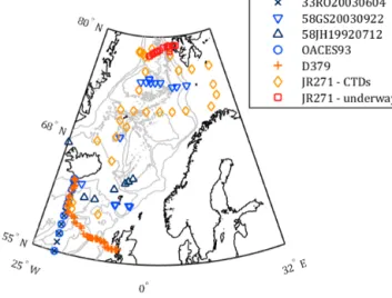
We present measurements of seawater δ¹³C_DIC from two cruises during summer 2012. The first cruise (RRS James Clark Ross, JR271) was carried out by the Sea Surface Consortium, part of the UK Ocean Acid- ification research programme (UKOA). These δ¹³C_DIC measurements will contribute towards quantifying the im- pact of ocean acidification upon the ocean carbon cycle and the biogeochemical processes which affect it, a high-level objective for this northeastern Atlantic/Nordic Seas cruise and the UKOA. The second cruise (RRS Discovery, D379) was a repeat occupation of the Extended Ellett Line (EEL) hydrographic transect in the northeastern Atlantic. These are the firstδ¹³CDICmeasurements made during an EEL cruise, establishing a baseline for future work on the transect. These cruises are located in an important region, partly overlapping with previous measurements but also filling a spatial gap in the existing global δ¹³C_DIC data set (Fig. 1; Schmittner et al., 2013).

2 Sample collection

2.1 Cruise details

Samples for δ¹³CDIC measurements were collected during two cruises. The first was RRS James Clark Ross cruise JR271, which took place in the period between 1 June and 2 July 2012 in the northeastern Atlantic and Nordic Seas (Leakey, 2012; https://www.bodc.ac.uk/data/information_

and_inventories/cruise_inventory/report/jr271.pdf). During JR271, the maximum depth sampled at most stations was shallower than 500 m, because the overall sampling strategy for that cruise and research programme involved assessment of ocean acidification on surface ocean biogeochemical processes. The underway surface water samples collected during JR271 were from a transect across the Fram Strait at approximately 79^◦N, the northernmost part of the cruise.

The underway seawater supply intake was at an approxi- mate water depth of 5 m. The second cruise was RRS Dis-

Figure 1. Sample locations for cruises D379 (orange plusses) and JR271 (CTD stations: gold diamonds; underway: red squares), along with nearby historical δ¹³C_DIC data locations from the Schmittner et al. (2013) compilation: cruises 33RO20030604 (dark-blue crosses), 58GS20030922 (blue inverted triangles), 58JH19920712 (dark-blue triangles) and OACES93 (blue circles).

Grey contours indicate bathymetry at 500 m intervals from the GEBCO_2014 grid, version 20141103, http://www.gebco.net.

covery cruise D379, which took place in the period between 31 July and 17 August 2012, in the northeastern Atlantic (Griffiths, 2012; https://www.bodc.ac.uk/data/information_

and_inventories/cruise_inventory/report/d379.pdf). The EEL transect covered by D379 runs from Scotland to Iceland via the Rockall Trough and plateau, and the northernmost section of the route (at 20^◦W) overlaps the northern end of the A16 World Ocean Circulation Experiment (WOCE) hydrographic transect. The samples collected during D379 cover the full water column depth range. For both cruises, the sample locations are illustrated by Fig. 1, and information about the number and types of samples collected is given in Table 1.

2.2 Collection and storage methods

Prior to sample collection, the containers were thoroughly rinsed with deionised water (Milli-Q water, Millipore,

> 18.2 mcm⁻¹). Samples were collected from the source (either Niskin bottle or underway seawater supply) via silicone tubing, following established best-practice protocols (Dickson et al., 2007; McNichol et al., 2010), as sum- marised in this section. The containers were thoroughly rinsed with excess sample directly before filling until over- flowing with seawater, taking care not to generate or trap any air bubbles. Two different sample containers were used, called “bottles” and “vials”: (1) 100 mL soda-lime glass “bottles” (Dixon Glass, UK) with ground glass stoppers, lubri- cated with Apiezon^®L grease and held shut with electrical tape; (2) 50 mL glass “vials” with plastic screw-cap lids and PTFE/silicone septa. A total of 0.02 % of the sample con-

(3)

Table 1.Quantities and types of samples collected during cruises JR271 and D379, and types of sample containers used. D379 duplicates where one sample was collected in each type of container are counted in the “Unique samples – Bottles” cell (asterisked). The row labelled

“Both (totals)” shows the total number of samples collected during both cruises.

Cruise CTD stations Underway Total

Bottles Vials Bottles

JR271 Unique samples 210 0 17 227

Incl. duplicates 221 0 17 238

D379 Unique samples 62^∗ 263 0 325

Both (totals) Unique samples 272 263 17 552

tainer volume of saturated mercuric chloride solution was added to sterilise each sample before sealing. A 1 mL air headspace (1 % of the sample volume) was also introduced into the bottles by removing 1 mL of seawater via pipette from the bottles when full of sample. This was to prevent thermal expansion and contraction of the seawater sample from damaging the bottle or breaking the airtight seal, following best practices for dissolved inorganic carbon samples collected in similar containers (Dickson et al., 2007). The vials had flexible septa, so they were instead sealed com- pletely full of seawater. All samples were stored in the dark until analysis.

3 Sample analysis

Theδ¹³C_DICsamples were analysed at the Scottish Univer- sities Environmental Research Centre Isotope Community Support Facility (SUERC-ICSF) in East Kilbride (UK), between June and August 2013.

3.1 Definitions

The abundance of¹³C relative to¹²C in a given substanceX is given by Eq. (1). For each sampleX,RXis then normalised to a reference standard using Eq. (2).

R_X= ₁₃

C

X

₁₂ C

X

, (1)

where [¹³C]X and [¹²C]Xare the concentrations of¹³C and

12C respectively inX.

δ¹³C=R_sample−R_standard Rstandard

×1000 ‰ (2)

3.2 Analysis procedure

Samples were analysed in a batch process. For each batch, δ¹³C was measured in 88 Exetainer^® glass vials, each of 12 mL volume. At least 18 vials per batch were set aside for

calibration standards (“standard vials”), while the rest were used for seawater samples (“sample vials”).

Most of the standards were analysed before any samples, at the start of each batch (“initial standards”), except for a pair near the middle and at the end (“mid-point standards”

and “end-point standards” respectively). Three SUERC- ICSF in-house standards (powdered carbonate/bicarbonate solids called MAB, NA and CA; see Table 2) were used to calibrate theδ¹³C_DICresults to the Vienna Pee Dee Belem- nite (V-PDB) international standard (Coplen, 1995). These in-house standards have previously been calibrated against the NBS 19 international standard. The initial standards con- sisted of a range of masses of all three of the in-house standards. The mid- and end-point standards, used for drift correction, were of similar mass and the same type (MAB for batches 1 and 2, and NA thereafter).

A total of 103 seawater samples were subsampled twice and analysed consecutively (“analysis duplicates”). This was carried out for all samples in the first two batches, and every 10th sample thereafter.

The analysis procedure for each batch was necessarily slightly different for the standards and samples because of their different states (solid and liquid respectively). The standard and sample vials were soaked and rinsed with deionised water, then dried overnight at 65^◦C. The calibration mate- rials were weighed into the standard vials, whilst 80 µL of concentrated phosphoric acid (mixed with phosphorus pentoxide to result in minimum 100 % saturation) was added to each sample vial in order to convert all of the dissolved carbonate and bicarbonate in the seawater sample (added later) into CO2. All vials were then closed using plastic screw-cap lids with PTFE/silicone septa to make an airtight seal. These lids were not removed until the entire analysis process was complete. All addition or removal of fluids from the vials after this point was via injection of a needle through the septa.

The air in each vial was replaced, to remove CO₂, by flush- ing with helium for 15 min (“overgassing”). This was an au- tomated process carried out by a CTC Analytics PAL system.

After overgassing, 1 mL of the phosphoric acid/phosphorus pentoxide diluted with deionised water to 10 % concentration

(4)

Table 2.The SUERC-ICSF in-house calibration standards. The certified values in the final column are the values taken byCin Eq. (4).

MAB, NA and CA are the names of the standards, and are not specific abbreviations/acronyms.

Name Chemical Certifiedδ¹³C composition V-PDB / ‰

MAB CaCO₃ +2.48

NA NaHCO₃ −4.67

CA CaCO₃ −24.23

was added to each standard vial. For each sample, a syringe was rinsed three times with the sample and then used to trans- fer 1 mL of that sample into the vial. All of the vials were then left for at least 24 h for the standard or sample to fully react with the acid and equilibrate with the gas headspace.

Finally, the gas headspace in each vial was automatically sampled by the PAL System, and theδ¹³C of the CO₂measured 10 times by a Thermo Scientific Delta V mass spec- trometer via a Thermo Scientific GasBench II. The set of 10 measurements for each sample or standard are henceforth re- ferred to as “technical replicates”.

4 Measurement processing

4.1 Batch-by-batch processing

The raw δ¹³C results were processed using MATLAB®

(MathWorks) software in five steps: (1) anomalous measurement removal, (2) averaging, (3) peak area correction, (4) calibration to V-PDB, and (5) drift correction. Except where specified, these steps were applied to each analysis batch independently, using only data from that specific batch.

4.1.1 Anomalous measurement removal

To begin, anomalousδ¹³C measurements were removed from the sets of technical replicates. These typically occurred when the CO₂ concentration in a replicate was too high or low, resulting in the peak area falling outside of the calibration range. Therefore, only measurements with a peak area between 10 and 145 were retained, and if fewer than 6 of the original 10 technical replicates for a given sample fell in the acceptable peak area range, the entire sample was discarded.

4.1.2 Averaging

After anomalous measurements were removed, the mean δ¹³C and peak area were calculated from each sample’s technical replicates. These mean values were used for the remain- der of the data processing.

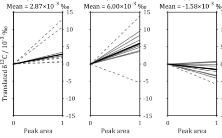
Figure 2.Peak area vs.δ¹³C relationships used for the peak area correction of the calibration standards (a) MAB, (b) NA and (c) CA (Table 2). The grey lines are the linear least-squares best fit for each analysis batch but are vertically translated to have ayintercept of 0, so that theyvalue of the line at a peak area of 1 is equal to the gradient. The thick black line is the mean gradient for each standard;

the dashed grey lines indicate batches excluded from calculation of the mean (see Sect. 4.1.3 for exclusion criteria).

4.1.3 Peak area correction

Plots of peak area against raw δ¹³C reveal relationships that are different for each of the three calibration standards (Fig. 2) and for seawater (Fig. 3). Peak area is controlled by CO₂concentration, so a range of peak areas can be generated by using a range of masses of calibration standards, or volumes of seawater, in different analyses, and these results can be used to quantify and correct for the relationships between peak area and rawδ¹³C. All corrections were linear and made to a peak area of 35, which is approximately equal to the mean peak area for all seawater samples across all analysis batches. For the calibration standards, the corrections were derived using the initial standards. For each batch, a linear least-squares regression between peak area and rawδ¹³C was derived for each standard. Regressions were discarded if the range of input peak areas either (i) did not include the value 35 or (ii) was smaller than 30. The mean gradient for each of the three standards (excluding discarded regressions) was then calculated across all batches and used to make the peak area correction for each standard (Fig. 2).

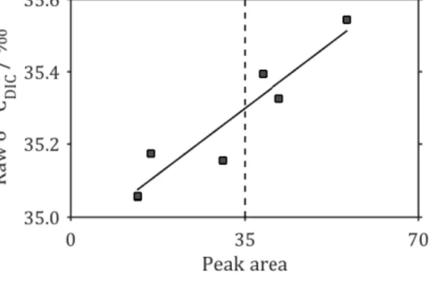
For the seawater samples, six subsamples of a large homogeneous seawater sample were taken in volumes from 0.50 to 1.50 mL (in 0.25 mL increments). These were measured consecutively during analysis batch #6, and a linear least-squares regression ofδ¹³C against peak area was used to make the linearity correction for all seawater samples from all batches (Fig. 3). All corrections were made using an equation of the form

δ_corr=δ_meas−g(A−35), (3)

whereδ_corris the correctedδ¹³C_DICvalue;δ_measis the original, uncorrectedδ¹³C_DICvalue;Ais the peak area; andgis

(5)

Figure 3.Peak area vs.δ¹³C relationship for homogeneous seawater sampled at a range of volumes from 0.5 to 1.5 mL (grey squares). The black best-fit line shows the relationship used to correct all seawater samples for peak area, and the vertical dashed line at (peak area)=35 indicates the peak area to which corrections have been made.

the appropriate correction gradient. For the standards MAB, NA and CA,gis 2.87×10⁻³, 6.00×10⁻³and−1.58×10⁻³ respectively (Fig. 2), while for the seawater samples, g is 1.04×10⁻²(Fig. 3).

4.1.4 Calibration to V-PDB

The mean of the peak-area-corrected δ¹³C for each of the three calibration standards was calculated (L), using only the measurements of the initial standards. A non-linear fit (Eq. 4) betweenLand the corresponding certified values relative to V-PDB (C, Table 2) was used to determine constants x, y andzfor each batch and then calibrate the samples to the V- PDB international standard (Coplen, 1995). The fit used an equation of the form

L²+C²+x·L+y·C+z=0. (4)

4.1.5 Drift correction

An interpolation between three points was used to correct for instrument drift during each batch. The index was the analysis position, with the mean analysis positions for the initial, mid-point and end-point standards as sample points for the interpolation. The initial point was assigned a value (drift) of 0, and mid-point and end-point values were calculated by subtracting the mean calibratedδ¹³C for each of the mid-point and end-point standard pairs from their certified values (Table 2). Piecewise cubic hermite interpolating polynomial (PCHIP) fits (Fritsch and Carlson, 1980; Kahaner et al., 1988) between analysis position and drift were generated and used to correct all results other than the initial standards.

4.2 Quality control

After calibration, the meanδ¹³C_DIC and its standard deviation (SD) were calculated for all seawater samples in all batches. Four of the 608 measurements had extremely low δ¹³C_DICvalues, more than 6 SDs away from the mean. These measurements were discarded; they are assumed to represent sample containers where the airtight seal failed and the DIC is thus contaminated with atmospheric CO₂, which has a much lowerδ¹³C than typical ocean DIC (Lynch-Stieglitz et al., 1995). Theδ¹³C_DICmeasurements were finally com- bined with their cruise metadata, using the mean values for pairs of analysis and sample duplicates, and the differences between the two samples in each duplicate pair calculated for statistical evaluation.

4.3 Data availability

The final, calibrated δ¹³C_DIC results have been archived with the British Oceanographic Data Centre and are publicly accessible, free of charge (Humphreys et al., 2014a, b;

data doi:10.5285/09760a3a-c2b5-250b-e053-6c86abc037c0, doi:10.5285/09511dd0-51db-0e21-e053-6c86abc09b95).

Measurements of additional hydrographic variables for cruise D379 are similarly available from the Carbon Diox- ide Information Analysis Center (Hartman et al., 2014;

http://cdiac.ornl.gov/ftp/oceans/CLIVAR/EllettLine/EEL_

2012_D379). Theδ¹³C_DICresults have also been submitted to an ongoing global compilation of seawaterδ¹³C_DICdata (Becker et al., 2015) as part of which they will undergo a secondary quality-control procedure.

4.4 Crossover analysis

A simple crossover analysis was performed to evaluate the consistency of our results with previous nearby results from the quality-controlled compilation ofδ¹³C_DICdata produced by Schmittner et al. (2013). First, all sampling stations in the Schmittner et al. (2013) data set within 150 km of a D357 or JR271 CTD station were selected. At each of our CTD sampling stations, a PCHIP was implemented by MAT- LAB (MathWorks) to interpolateδ¹³C_DICto the same depths that the nearby Schmittner et al. (2013)δ¹³C_DICdata were from. Using only data from deeper than 1500 m to minimise the confounding effect of seasonal variability, our interpo- latedδ¹³CDICvalues were subtracted from the results at the same depth from Schmittner et al. (2013) in order to give the δ¹³CDIC residuals. Finally, the mean and SD of all of theseδ¹³CDICresiduals were calculated for each Schmittner et al. (2013) cruise.

(6)

Table 3.Summary of the anomalous measurement removal process for all of the seawater samples. Numbers in each row are for all data after application of the measurement removal step indicated in the first column. Tech. rep. SD: standard deviation of uncalibratedδ¹³C_DIC, calculated for each sample’s set of 10 technical replicates.

Measurement Number of Number of Mean tech. Max. tech.

removal step measurements sample sets rep. SD / ‰ rep. SD / ‰

All raw data 7410 741 0.240 66.60

10 < peak area < 145 7349 740 0.029 0.616

Valid tech. reps≥6 7329 734 0.028 0.058

5 Discussion and statistics

5.1 Anomalous measurement removal

The process of removing anomalous measurements from the raw data eliminated approximately 1 % of the seawater sample technical replicates, but reduced the mean and maximum SD of these sets of replicates by one and three orders of magnitude respectively. Limiting the range of acceptable peak areas was responsible for almost all of the reduction in the mean SD and significantly reduced the maximum SD. Inter- mittent very low peak areas were suspected to be a conse- quence of transient liquid blockages in the tubing that drew the gaseous samples from the vials into the mass spectrome- ter. The second step of discarding samples with fewer than six technical replicates in this acceptable peak area range made little difference to the mean SD, but resulted in a fur- ther reduction to the maximum SD by an order of magnitude (Table 3). Figure 4 illustrates the SD of all sets of technical replicates for samples throughout the analysis.

5.2 Calibration to V-PDB

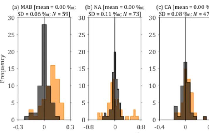
Initially, a linear fit was tested to calibrate the rawδ¹³C measurements to the V-PDB standard. An initial check on the quality of the calibration is to apply it to the standards that it was generated from, which should return near-perfect results (i.e. the certified values for each standard). However, this was not the case: the linear calibration returnedδ¹³C values that were higher than the certified values for MAB and CA standards, and values that were lower than certified for NA. These over/underestimations were consistent in polarity across all batches, with mean values of +0.08, −0.10 and +0.03 ‰ for MAB, NA and CA respectively (Fig. 5). This was therefore easily resolved by using a non-linear calibration fit. A circular fit (Eq. 4) was used, rather than an ordinary polynomial, because it maintains constant curvature in the calibration space, which has the same units of per mille (‰) on both axes. With the non-linear fit, for all standards across all 11 batches, the mean±SD of the difference between calibrated and certifiedδ¹³C was 0.00±0.06 ‰ (MAB, 59 analyses), 0.00±0.11 ‰ (NA, 73 analyses) and 0.00±0.08 ‰ (CA, 47 analyses) (Fig. 5), a notable improvement.

Figure 4.Standard deviation (SD) of technical replicates for each seawater sample, after anomalous peak removal. Alternating black and grey sections indicate separate analysis batches.

Figure 5.Distributions of the difference between calibrated and certifiedδ¹³C for calibration standards (a) MAB, (b) NA and (c) CA (Table 2) in all batches. The orange histograms indicate the distributions resulting from using a linear calibration equation, while the overlying black-grey histograms show the improved distributions from the non-linear calibration that we used instead (Eq. 4).

SD: standard deviation;N: number of analyses, both in reference to the black-grey histograms, which represent the actual calibration used.

5.3 Repeatability from duplicates

Comparison with published estimates of uncertainty for δ¹³C_DICmeasurements is complicated by the various different definitions used in the literature. In this study, the mean

(7)

Table 4.Mean absolute differences between sampling duplicates.

The “sample container” column indicates whether the duplicates were collected in the same type of container as each other, or different containers (i.e. one in a vial, one in a bottle).

Cruise Sample Number Mean absolute container of pairs difference / ‰

D379 Same 16 0.109

JR271 Same 11 0.080

Both Same 27 0.097

D379 Different 9 0.168

absolute difference in calibrated δ¹³CDIC for all analytical duplicate pairs was 0.053 ‰. This is very close to published values which we believe to be equivalently defined. For example, Olsen et al. (2006) quote a long-term precision for δ¹³C, based on replicates, of 0.05 ‰.

To evaluate the true measurement repeatability, including error introduced by the sampling process, it is necessary to use the sample duplicates rather than the analytical duplicates (Table 4). The mean duplicate pair difference for samples in the same type of container across both cruises was 0.097 ‰.

However, where the duplicate samples were collected in different containers (one in a bottle, one in a vial), the mean absolute duplicate pair difference took the higher value of 0.168 ‰. This suggests that the differences in the sampling method for the different containers introduced a measurable increase in the uncertainty. To test whether there was a systematic offset inδ¹³CDICmeasured in the different container types, we subtracted the vial value from the bottle value for these duplicate pairs with non-matching containers and performed a one-sample t test for the null hypothesis that the resulting distribution had a mean value of 0. It was not possible to reject the null hypothesis at the 95 % certainty level, so we did not find a consistent offset between the container types.

The expected SD of a large number of measurements of the same sample (i.e. the 1σ uncertainty or precision) can be estimated from the mean duplicate pair absolute difference by dividing by 2/√

π (Thompson and Howarth, 1973). For this study, for the duplicates from both cruises which were in the same type of container, the precision defined in this way is 0.09 ‰. As these duplicate pairs were always measured consecutively in the same batch as each other, this is a value that indicates the short-term reproducibility (i.e. repeatability) of our measurements, and does not include any additional differences that may or may not exist between analysis batches. Like the analytical repeatability, this compares well with equivalent published values. For example, Olsen et al. (2006) found an SD of 0.07 ‰ for 16 samples taken in seawater with “very similar physical and chemical water mass characteristics”; Quay et al. (2007) reported a “reproducibility... based on replicate measurements” of ±0.03 ‰

; McNichol et al. (2010) record a “replication” of±0.03 ‰

Figure 6.Measuredδ¹³C_DIC/ ‰ for all samples from both cruises collected at a depth shallower than 10 m. Actual sampling points are indicated by black plusses.

Figure 7.Measuredδ¹³C_DIC/ ‰ for all samples from cruise D379.

Actual sampling points are indicated by black plusses. Section runs from Iceland to Scotland from left to right; see Fig. 1 for precise route. Bathymetry data are from the GEBCO_2014 grid, version 20141103, http://www.gebco.net, and are approximate to the cruise route.

(8)

from measurements of duplicate seawater samples from the Niskin bottle; and Griffith et al. (2012) calculated a “pooled SD” for eight duplicateδ¹³C_DICsamples of 0.23 ‰. In con- clusion, the uncertainty of our measurements falls within the range of previously published results.

5.4 Results distribution

The measuredδ¹³C_DICvalues during both cruises (D379 and JR271) are illustrated by Figs. 6 and 7. All of the δ¹³C_DIC measurements were in the range from −0.58 to+2.37 ‰, relative to V-PDB.

Crossover analysis

The simple crossover analysis (Sect. 4.4) found that any systematic offsets between our measurements and those in the Schmittner et al. (2013) compilation were negligible. Two cruises from the compilation met the criteria of having δ¹³C_DIC data deeper than 1500 m within a lateral distance of 150 km of a D357 or JR271 station:

OACES93 and 58GS20030922 (Fig. 1). For OACES93, crossovers were possible with stations from both D357 and JR271, while for 58GS20030922 there were only crossovers with JR271. Overall, the means±SDs of the δ¹³CDICresiduals were 0.07±0.09 ‰ for OACES93 (based on 36 matchingδ¹³CDICmeasurements) and 0.00±0.06 ‰ for 58GS20030922 (based on 10 matches). We therefore conclude that any systematic offset between our results and nearby historical data was negligible, relative to our measurement repeatability of 0.09 ‰, and to the accuracy of 0.1 to 0.2 ‰ estimated by Schmittner et al. (2013) for their compilation ofδ¹³C_DICdata.

Author contributions. M. P. Humphreys, E. P. Achterberg and A. M. Griffiths determined sampling strategy and collected the samples. M. P. Humphreys, A. McDonald and A. J. Boyce carried out the measurements and data processing. M. P. Humphreys prepared the manuscript with contributions from all co-authors.

Acknowledgements. We are grateful to the officers and crew of RRS James Clark Ross and RRS Discovery along with the science team on board both cruises for their support. We acknowledge funding by the Natural Environment Research Council for the PhD studentship to M. P. Humphreys (NE/J500112/1) and funding the carbon isotope analyses (IP/1358/1112), and the UKOA and EEL projects for funding and ship time (NE/H017348/1). We thank M. Ribas-Ribas, E. Tynan and V. M. C. Rérolle for assisting with sample collection on cruise JR271, and D. Wolf-Gladrow, A. Yool and the two anonymous reviewers for their constructive comments and advice.

Edited by: D. Carlson

References

Becker, M., Tanhua, T., Humphreys, M. P., Erlenkeuser, H., Ander- sen, N., and Körtzinger, A.: An internally consistent collection of oceanδ¹³C data, in preparation, 2015.

Brewer, P. G.: Direct observation of the oceanic CO₂increase, Geo- phys. Res. Lett., 5, 997–1000, doi:10.1029/GL005i012p00997, 1978.

Caldeira, K. and Wickett, M. E.: Anthropogenic carbon and ocean pH, Nature, 425, 365–365, doi:10.1038/425365a, 2003.

Chen, G.-T. and Millero, F. J.: Gradual increase of oceanic CO₂, Nature, 277, 205–206, doi:10.1038/277205a0, 1979.

Coplen, T. B.: Reporting of stable carbon, hydrogen, and oxygen isotopic abundances, in Reference and intercomparison materi- als for stable isotopes of light elements, Proceedings of a consul- tants meeting held in Vienna, 1–3 December 1993, International Atomic Energy Agency, 1995.

Dickson, A. G., Sabine, C. L., and Christian, J. R.: Guide to best practices for ocean CO₂measurements, PICES Special Publica- tion 3, TN, USA, 2007.

Doney, S. C., Fabry, V. J., Feely, R. A., and Kleypas, J. A.: Ocean Acidification: The Other CO₂Problem, Annu. Rev. Marine Sci., 1, 169–192, doi:10.1146/annurev.marine.010908.163834, 2009.

Fritsch, F. and Carlson, R.: Monotone Piecewise Cubic Interpola- tion, SIAM J. Numer. Anal., 17, 238–246, doi:10.1137/0717021, 1980.

Griffith, D. R., McNichol, A. P., Xu, L., McLaughlin, F. A., Mac- donald, R. W., Brown, K. A., and Eglinton, T. I.: Carbon dy- namics in the western Arctic Ocean: insights from full-depth carbon isotope profiles of DIC, DOC, and POC, Biogeosciences, 9, 1217–1224, doi:10.5194/bg-9-1217-2012, 2012.

Griffiths, C. R. (Ed.): RRS Discovery cruise D379, Southampton to Reykjavik, Extended Ellett Line, Scottish Association for Marine Science, Oban, UK, 184 pp., 2012.

Gruber, N., Sarmiento, J. L., and Stocker, T. F.: An improved method for detecting anthropogenic CO₂in the oceans, Global Biogeochem. Cy., 10, 809–837, doi:10.1029/96GB01608, 1996.

Hall, T. M., Haine, T. W. N., and Waugh, D. W.: In- ferring the concentration of anthropogenic carbon in the ocean from tracers, Global Biogeochem. Cy., 16, 1131, doi:10.1029/2001GB001835, 2002.

Hartman, S., Griffiths, A., and Achterberg, E.: Discrete Car- bon Dioxide Data Obtained During the R/V Discovery EEL_2012_D379 Cruise Along Extended Ellett Line, Carbon Dioxide Information Analysis Center, Oak Ridge National Lab- oratory, US Department of Energy, Oak Ridge, Tennessee, USA, doi:10.3334/CDIAC/OTG.CLIVAR_EEL_2012_D379, 2014.

Humphreys, M. P., Achterberg, E. P., Griffiths, A. M., McDonald, A., and Boyce, A.: Ellett Line measurements of the stable isotope composition of dissolved inorganic carbon in the Northeastern Atlantic and Nordic Seas during summer 2012, British Oceano- graphic Data Centre, Natural Environment Research Coun- cil, UK, doi:10.5285/09760a3a-c2b5-250b-e053-6c86abc037c0, 2014a.

Humphreys, M. P., Achterberg, E. P., Griffiths, A. M., McDonald, A., and Boyce, A.: UKOA measurements of the stable isotope composition of dissolved inorganic carbon in the Northeastern Atlantic and Nordic Seas during summer 2012, British Oceano- graphic Data Centre, Natural Environment Research Coun-

(9)

cil, UK, doi:10.5285/09511dd0-51db-0e21-e053-6c86abc09b95, 2014b.

Kahaner, D., Moler, C., and Nash, S.: Numerical Methods and Soft- ware, Prentice Hall, NJ, USA, 1988.

Keeling, C. D.: The Suess effect:¹³Carbon-¹⁴Carbon interrelations, Environ. Int., 2, 229–300, doi:10.1016/0160-4120(79)90005-9, 1979.

Khatiwala, S., Primeau, F., and Hall, T.: Reconstruction of the his- tory of anthropogenic CO₂concentrations in the ocean, Nature, 462, 346–349, doi:10.1038/nature08526, 2009.

Leakey, R. J. G. (Ed.): UK Ocean Acidification Research Pro- gramme Arctic Cruise Report, Scottish Association for Marine Science, Oban, UK, 310 pp., 2012.

Le Quéré, C., Raupach, M. R., Canadell, J. G., Marland, G., Bopp, L., Ciais, P., Conway, T. J., Doney, S. C., Feely, R. A., Foster, P., Friedlingstein, P., Gurney, K., Houghton, R. A., House, J. I., Huntingford, C., Levy, P. E., Lomas, M. R., Majkut, J., Metzl, N., Ometto, J. P., Peters, G. P., Prentice, I. C., Randerson, J. T., Run- ning, S. W., Sarmiento, J. L., Schuster, U., Sitch, S., Takahashi, T., Viovy, N., van der Werf, G. R., and Woodward, F. I.: Trends in the sources and sinks of carbon dioxide, Nature Geosci., 2, 831–836, doi:10.1038/ngeo689, 2009.

Lynch-Stieglitz, J., Stocker, T. F., Broecker, W. S., and Fairbanks, R. G.: The influence of air-sea exchange on the isotopic composition of oceanic carbon: Observations and modeling, Global Biogeochem. Cy., 9, 653–666, doi:10.1029/95GB02574, 1995.

McNeil, B. I., Matear, R. J., and Tilbrook, B.: Does carbon 13 track anthropogenic CO₂in the southern ocean?, Global Biogeochem.

Cy., 15, 597–613, doi:10.1029/2000GB001352, 2001.

McNichol, A., Quay, P. D., Gagnon, A. R., and Burton, J. R.: Col- lection and measurement of carbon isotopes in seawater DIC, in The GO-SHIP Repeat Hydrography Manual: A Collection of Expert Reports and Guidelines, IOCCP Report NO. 14, ICPO Publication Series No. 134, Version 1, available at: http://www.

go-ship.org/HydroMan.html (last access: 12 June 2015), 2010.

Olsen, A., Omar, A. M., Bellerby, R. G. J., Johannessen, T., Ninne- mann, U., Brown, K. R., Olsson, K. A., Olafsson, J., Nondal, G., Kivimäe, C., Kringstad, S., Neill, C., and Olafsdottir, S.: Mag- nitude and origin of the anthropogenic CO₂ increase and¹³C Suess effect in the Nordic seas since 1981, Global Biogeochem.

Cy., 20, GB3027, doi:10.1029/2005GB002669, 2006.

Quay, P. D., Tilbrook, B., and Wong, C. S.: Oceanic Uptake of Fossil Fuel CO₂: Carbon-13 Evidence, Science, 256, 74–79, doi:10.1126/science.256.5053.74, 1992.

Quay, P., Sonnerup, R., Westby, T., Stutsman, J., and McNichol, A.: Changes in the¹³C/¹²C of dissolved inorganic carbon in the ocean as a tracer of anthropogenic CO₂uptake, Global Bio- geochem. Cy., 17, GB1004, doi:10.1029/2001GB001817, 2003.

Quay, P. D., Sonnerup, R., Stutsman, J., Maurer, J., Körtzinger, A., Padin, X. A., and Robinson, C.: Anthropogenic CO₂accumulation rates in the North Atlantic Ocean from changes in the 13C/¹²C of dissolved inorganic carbon, Global Biogeochem. Cy., 21, GB1009, doi:10.1029/2006GB002761, 2007.

Sabine, C. L. and Tanhua, T.: Estimation of Anthropogenic CO₂ Inventories in the Ocean, Annu. Rev. Marine Sci., 2, 175–198, doi:10.1146/annurev-marine-120308-080947, 2010.

Sabine, C. L., Feely, R. A., Gruber, N., Key, R. M., Lee, K., Bullis- ter, J. L., Wanninkhof, R., Wong, C. S., Wallace, D. W. R., Tilbrook, B., Millero, F. J., Peng, T.-H., Kozyr, A., Ono, T., and Rios, A. F.: The Oceanic Sink for Anthropogenic CO₂, Science, 305, 367–371, doi:10.1126/science.1097403, 2004.

Schmittner, A., Gruber, N., Mix, A. C., Key, R. M., Tagliabue, A., and Westberry, T. K.: Biology and air-sea gas exchange controls on the distribution of carbon isotope ratios (δ¹³C) in the ocean, Biogeosciences, 10, 5793–5816, doi:10.5194/bg-10-5793-2013, 2013.

Sonnerup, R. E. and Quay, P. D.: ¹³C constraints on ocean carbon cycle models, Global Biogeochem. Cy., 26, GB2014, doi:10.1029/2010GB003980, 2012.

Sonnerup, R. E., Quay, P. D., McNichol, A. P., Bullister, J.

L., Westby, T. A., and Anderson, H. L.: Reconstructing the oceanic¹³C Suess Effect, Global Biogeochem. Cy., 13, 857–872, doi:10.1029/1999GB900027, 1999.

Sonnerup, R. E., McNichol, A. P., Quay, P. D., Gammon, R. H., Bullister, J. L., Sabine, C. L., and Slater, R. D.: Anthropogenic δ¹³C changes in the North Pacific Ocean reconstructed using a multiparameter mixing approach (MIX), Tellus B, 59, 303–317, doi:10.1111/j.1600-0889.2007.00250.x, 2007.

Tanhua, T., Körtzinger, A., Friis, K., Waugh, D. W., and Wallace, D.

W. R.: An estimate of anthropogenic CO₂inventory from decadal changes in oceanic carbon content, P. Natl. Acad. Sci. USA, 104, 3037–3042, doi:10.1073/pnas.0606574104, 2007.

Thompson, M. and Howarth, R. J.: The rapid estimation and control of precision by duplicate determinations, Analyst, 98, 153–160, doi:10.1039/AN9739800153, 1973.