Stable carbon isotopes of dissolved inorganic carbon for a zonal transect across the subpolar North Atlantic

(1)

www.earth-syst-sci-data.net/8/221/2016/

doi:10.5194/essd-8-221-2016

Stable carbon isotopes of dissolved inorganic carbon for a zonal transect across the subpolar North Atlantic

Ocean in summer 2014

Matthew P. Humphreys¹, Florence M. Greatrix¹, Eithne Tynan¹, Eric P. Achterberg^1,2, Alex M. Griffiths³, Claudia H. Fry¹, Rebecca Garley⁴, Alison McDonald⁵, and Adrian J. Boyce⁵

1Ocean and Earth Science, University of Southampton, Southampton, UK

2GEOMAR Helmholtz Centre for Ocean Research, Kiel, Germany

3Department of Earth Science and Engineering, Imperial College London, London, UK

4Bermuda Institute of Ocean Sciences, St George’s, Bermuda

5Scottish Universities Environmental Research Centre, East Kilbride, UK Correspondence to:Matthew P. Humphreys (m.p.humphreys@soton.ac.uk) Received: 10 November 2015 – Published in Earth Syst. Sci. Data Discuss.: 9 March 2016

Revised: 16 May 2016 – Accepted: 17 May 2016 – Published: 3 June 2016

Abstract. The stable carbon isotope composition of dissolved inorganic carbon (δ¹³C_DIC) in seawater was measured in samples collected during June–July 2014 in the subpolar North Atlantic. Sample collection was carried out on the RRSJames Clark Rosscruise JR302, part of the “Radiatively Active Gases from the North Atlantic Region and Climate Change” (RAGNARoCC) research programme. The observedδ¹³CDIC values for cruise JR302 fall in a range from−0.07 to+1.95 ‰, relative to the Vienna Pee Dee Belemnite standard. From duplicate samples collected during the cruise, the 1σ precision for the 341 results is 0.08 ‰, which is similar to our previous work and other studies of this kind. We also performed a cross-over analysis using nearby historical δ¹³CDICdata, which indicated that there were no significant systematic offsets between our measurements and previously published results. We also included seawater reference material (RM) produced by A. G. Dickson (Scripps Institution of Oceanography, USA) in every batch of analysis, enabling us to improve upon the calibration and quality-control procedures from a previous study. Theδ¹³C_DICis consistent within each RM batch, although its value is not certified. We reportδ¹³C_DICvalues of 1.15±0.03 ‰ and 1.27±0.05 ‰ for batches 141 and 144 respectively. Our JR302δ¹³C_DICdata can be used – along with measurements of other biogeochemical variables – to constrain the processes that control DIC in the interior ocean, in particular the oceanic uptake of anthropogenic carbon dioxide and the biological carbon pump. Ourδ¹³C_DICresults are available from the British Oceanographic Data Centre – doi:10.5285/22235f1a-b7f3-687f-e053-6c86abc0c8a6.

1 Introduction

The global ocean has absorbed up to half of the anthropogenic carbon dioxide (CO₂) emitted since the early 1800s (Sabine et al., 2004; Khatiwala et al., 2009, 2013) and it con- tinues to take up about a quarter of annual CO₂emissions at the present day (Le Quéré et al., 2009), substantially decreas- ing CO₂accumulation in the atmosphere. The consequences of this uptake include a decline in pH – known as ocean acidification – with lower pH values predicted to persist for cen-

turies longer than the atmospheric CO₂anomaly (Caldeira and Wickett, 2003), which will have impacts on marine biogeochemistry and ecology that we are only just beginning to understand (Doney et al., 2009; Achterberg, 2014; Gaylord et al., 2015).

In order to predict the response of the oceanic CO2sink to the continuing rise of the atmospheric partial pressure of CO2(pCO2), it is useful to first understand the existing spatial distribution of anthropogenic dissolved inorganic carbon (DIC_anth) in the ocean interior. Various methods have

(2)

been employed to this end (Sabine and Tanhua, 2010), including back-calculation from DIC, total alkalinity (TA) and dissolved oxygen observations (Brewer, 1978; Chen and Millero, 1979; Gruber et al., 1996); inference from the oceanic distributions of other anthropogenic gases such as chlorofluorocarbons (Hall et al., 2002; Waugh et al., 2006);

and multi-linear regressions using measurements from pairs of cruises in the same region, but separated in time (Friis et al., 2005; Tanhua et al., 2007). Oceanic measurements during the past few decades (Quay et al., 2007) and over longer timescales in ice cores (Rubino et al., 2013) show that the rise inpCO2and DIC has been accompanied by a decline in the carbon-13 content of DIC, relative to carbon-12 (reported asδ¹³C, Eqs. 1 and 2), a phenomenon called the “Suess effect” (Keeling, 1979). This is caused by the lower δ¹³C of anthropogenic CO2relative to pre-industrial and present-day atmospheric CO₂, and it provides another approach to constrain the spatial distribution and inventory of anthropogenic DIC (e.g. Quay et al., 1992, 2003, 2007; Sonnerup et al., 1999, 2007; Körtzinger et al., 2003). The Suess effect has caused significant changes in the present-day distribution of δ¹³C_DICin the ocean interior (Olsen and Ninnemann, 2010).

Continued observations of oceanicδ¹³C_DICare essential for verification of the parameterisations of ocean carbon cycle models (Sonnerup and Quay, 2012).

Here, we present measurements ofδ¹³C_DICfrom a zonal transect across the subpolar North Atlantic Ocean in June–

July 2014. The cruise, JR302 on the RRS James Clark Ross, was carried out as part of the “Radiatively Active Gases from the North Atlantic Region and Climate Change”

(RAGNARoCC) research programme. Our observations fill important spatiotemporal gaps in the existing global data set (Schmittner et al., 2013), and will contribute towards the scientific objectives summarised above. Our analysis was carried out following the methodology presented by Humphreys et al. (2015a), but we have been able to make several improvements to the raw data processing and calibration procedures by inclusion of seawater reference material (RM) in every batch of sample analysis. This RM, produced by A.

G. Dickson (Scripps Institution of Oceanography, USA), is mainly used for assessing the accuracy of non-isotopic marine carbonate chemistry measurements, and it does not have a certifiedδ¹³CDICvalue. Nevertheless, theδ¹³CDICof different RM bottles from the same RM batch should be consistent, allowing us to assess the consistency of our measurements between analysis batches. We determineδ¹³CDICvalues for the two RM batches that we measured (141 and 144), which could be used to check for systematic offsets between our results and those from other laboratories. We also use the RM results to carry out a statistical analysis of our measurement precision both within and between analysis batches.

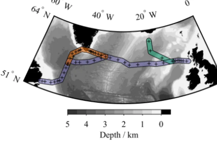
Figure 1.Bathymetric map of the subpolar North Atlantic Ocean.

Black plusses show δ¹³C_DIC sampling locations during cruise JR302. Coloured sections indicate illustrated transects: blue for Fig. 6, orange for Fig. 7, and green for Fig. 8. Bathymetry data are from the GEBCO_2014 grid, version 20150318, http://www.gebco.

net.

2 Sample collection

2.1 Cruise details

The δ¹³C_DIC samples were collected during RRS James Clark Rosscruise JR302, which was an approximately zonal transect from St John’s, Newfoundland, Canada, to Imming- ham, UK (Fig. 1), from June to July 2014 (King and Holli- day, 2015). During the crossing, several transects were sailed in towards the coast of Greenland, and in the eastern region the ship carried out a short meridional transect north towards Iceland in order to sample the Extended Ellett Line (Holliday and Cunningham, 2013).

2.2 Sample collection and storage

Prior to sample collection, the containers were thoroughly rinsed with deionised water (Milli-Q water, Millipore,

>18.2 mcm⁻¹). Samples were collected from the source (either seawater sampling bottle or underway seawater sup- ply) via silicone tubing, following established best-practice protocols (Dickson et al., 2007; McNichol et al., 2010), as summarised here. The containers were thoroughly rinsed with excess seawater sample immediately before filling until overflowing with seawater, taking care not to generate or trap air bubbles. Two different sample containers were used:

(1) 100 mL glass “bottles” with ground glass stoppers, lu- bricated with Apiezon^® L grease and held shut with elec- trical tape, and (2) 50 mL glass “vials”, with plastic screw- cap lids and PTFE/silicone septa. In order to sterilise each sample, 0.02 % of the sample container volume of saturated mercuric chloride solution was added before sealing. A 1 mL air headspace (i.e. 1 % of the sample volume) was also in- troduced to the bottles, prior to poisoning, by removing this

(3)

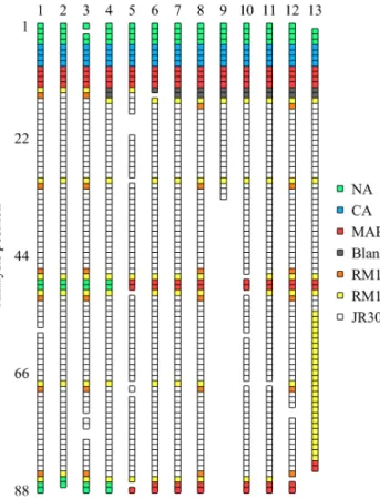
Figure 2.Schematic arrangement of calibration standards (NA, CA and MAB), blanks, RM and samples (JR302) within each analysis batch. Each square represents a separate measurement (i.e. a set of 10 technical replicates). Gaps are left where results have failed quality control.

volume of seawater via pipette. This prevents thermal expan- sion/contraction of the seawater from breaking the airtight seal. However, the flexible septa on the vials allowed them to be sealed when full of seawater. All samples were stored in the dark until analysis.

3 Sample analysis

All of the δ¹³CDIC samples were analysed at the Scottish Universities Environmental Research Centre Isotope Com- munity Support Facility (SUERC-ICSF) in East Kilbride (UK), in June–July 2015. We describe the analysis procedure here only in brief, as it was identical to that of Humphreys et al. (2015a).

The samples were analysed in 13 batches. Each analysis batch consisted of up to 88 measurements, 16 of which were of calibration standards, and the remainder were of seawater samples, “blanks” or RM (Fig. 2). Each batch underwent a three-step process of overgassing, equilibration and measurement. For the overgassing step, the air in each of the measurement vials (12 mL Exetainer^®) was flushed out and replaced with helium by a PAL system (CTC Analytics). For

equilibration, the standards, samples and RM were reacted with phosphoric acid to convert all DIC to CO₂. Finally, the gaseous headspace in each measurement vial was then sam- pled by the PAL system and transferred to a Thermo Sci- entific Delta V mass spectrometer via a Thermo Scientific GasBench II, and was measured 10 times (called technical replicates).

For seawater samples and RM, four drops of concentrated phosphoric acid were added to the Exetainer analysis vials prior to overgassing, and 1 mL of liquid sample was then in- jected into each vial for equilibration. For the standards, only the solid powder standard was added to the analysis vials prior to overgassing, and 1 mL of dilute (10 % by volume) phosphoric acid was added to each vial for equilibration.

During batches 4 and 6–13, “blanks” were prepared in the same way as the standards, except that the Exetainer analysis vials were completely empty for overgassing, and had the same dilute acid added as the standards in that batch.

4 Measurement processing

We were able to make improvements to the processing of the raw measurements from our previous study (Humphreys et al., 2015a), in part by using the results from the RM that were included in every batch. The processing sequence used in this study is described in full here, including parts that are the same as in Humphreys et al. (2015a); differences between the two approaches are then discussed later. All processing was carried out using MATLAB^®(MathWorks, USA).

4.1 Definitions

The relative abundance of¹³C to¹²C in a sampleXis given by Eq. (1). TheR_Xis then normalised to a reference standard – i.e. Vienna Pee Dee Belemnite (V-PDB) (Coplen, 1995) – using Eq. (2).

R_X= ₁₃

C

X

₁₂ C

X

, (1)

where [¹³C]_Xand [¹²C]_Xare the concentrations of¹³C and

12C respectively inX.

δ¹³C=R_sample−R_V−PDB RV−PDB

×1000 ‰ (2)

4.2 General procedure

4.2.1 Anomalous measurement removal

Anomalousδ¹³C measurements were first removed from the sets of technical replicates. These typically occurred when the CO₂ concentration in a replicate was too low, causing the peak area to fall outside the calibrated range (i.e. the range of peak areas covered by the standards). There were no

(4)

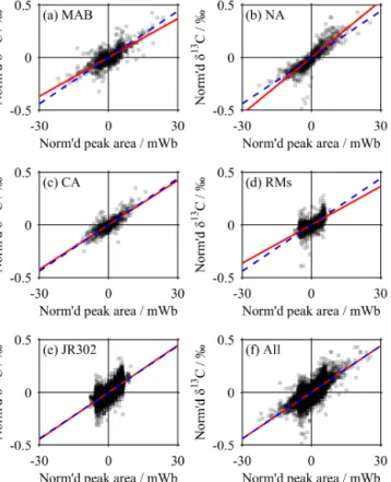
Figure 3.The peak area correction relationship. All technical replicates are plotted, normalised such that the mean peak area andδ¹³C for each set of technical replicates are both 0 (‰ or mWb respectively). The red line is the same in each plot, showing the mean relationship used for all of the peak area corrections, while each dashed blue line shows the equivalent relationship determined only from the data scattered in each panel. Individual data points are semi- transparent.

sample measurements with peak areas greater than the calibrated range. Thus all measurements with a peak area less than 5 mWb were judged to be anomalous and discarded, and if this applied to 5 or more of the original 10 technical replicates for a given sample, the entire sample was discarded.

4.2.2 Peak area (linearity) correction

Virtually all samples, standards and RM showed a consistent decline in both peak area and raw δ¹³C through each set of technical replicates, called “linearity” (Fig. 3). To cor- rect for this, we first “normalised” the peak area and raw δ¹³C of each set of technical replicates by subtracting the mean peak area andδ¹³C respectively from each replicate;

every set of technical replicates thus had a mean normalised peak area andδ¹³C of 0 (mWb or ‰ respectively). We then performed an ordinary least-squares linear regression of nor- malisedδ¹³C against normalised peak area using all technical replicates from all of the samples, standards and RM. The regression was forced through the origin and had a gradient

(L) of 0.0147 ‰ mWb⁻¹. This was used to make a “peak area correction” to all technical replicates:

δ_lin=δ_raw−L(a−A_lin), (3) where δ_lin is the linearity-corrected δ¹³C, δ_raw is the raw δ¹³C measurement, L is the correction gradient (i.e.

0.0147 ‰ mWb⁻¹),ais the peak area for the technical replicate in mWb, andA_lin is 20 mWb – the peak area that the correction is made to. The value ofA_linwas chosen because it is the mean peak area for all of the seawater samples, thus minimising the magnitude of this correction.

4.2.3 Averaging

After the peak area correction had been applied, the mean δ¹³C of each set of technical replicates was calculated. These mean values were then used for the remainder of the data processing.

4.2.4 Blank correction

A “blank correction” was then applied to the standards only (MAB, NA and CA). This was necessary because phosphoric was added to these after the overgassing step, so any CO₂dissolved in the acid would be included in the measurement. It was not necessary for the seawater samples and RM, because here the acid was added prior to overgassing. The different procedures were necessary because of the different states of the standards and samples (solid and liquid respectively).

A pair of “blank” measurements were included during analysis batches 4 and 6–13. These were clean, empty Ex- etainer analysis vials that were otherwise treated in the same way as the standards: acid had been added after overgassing. The mean ± standard deviation (SD) peak area and linearity-corrected δ¹³C of all of these blanks were 0.277±0.024 mWb and 19.42±2.47 ‰ respectively. These mean values were then used to make the blank correction to all standards:

δ_blank=aδlin−AblankDblank

a−A_blank , (4)

where δblank is the blank-corrected δ¹³C, and Ablank and Dblank are the mean blank peak area and δ¹³C (i.e.

0.277±0.024 mWb and 19.42±2.47 ‰ respectively).

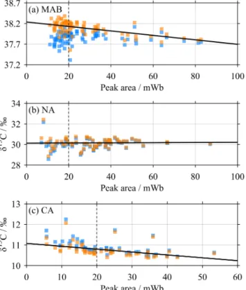
Even after this blank correction, there remained unexplained relationships between peak area and δ¹³C for the standards (Fig. 4). We therefore performed an ordinary least- squares regression between peak area and blank-corrected δ¹³C for all measurements in all analysis batches of each standard, and took the value of the regression line at a peak area of 20 mWb as theδ¹³C value for that standard in order to generate the V-PDB calibration curve (Table 1).

(5)

Figure 4.The blank correction for the standards. Each panel shows relationships between peak area and δ¹³C for(a)MAB,(b) NA and(c)CA before (blue) and after (orange) blank correction. The solid black lines are linear least-squares regressions for the data after blank correction. Their intercepts with the dashed black lines at 20 mWb were used as the mean values for each standard to generate the V-PDB calibration curve (Fig. 5). Note that the panels have different axes resolutions.

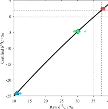
4.2.5 Calibration to V-PDB

A second-order polynomial fit was generated to determine the certifiedδ¹³C values for the standards (Table 1) from their blank-corrected mean values (Fig. 5):

δ_cert=cδ_blank² +sδ_blank+f, (5)

whereδcertis the certifiedδ¹³C value (Table 1) andc,sand f are coefficients describing the curvature, stretch and offset respectively of the calibration fit, taking the following values:

c= −4.321×10⁻³‰⁻¹, s=1.189, and f= −36.563 ‰.

Equation (5) was then used to calibrate all of the sample and RM measurements, by inputting the linearity-corrected δ¹³C values asδ_blank; the output (δ_cert) gives the final, cali- bratedδ¹³C_DIC, relative to the V-PDB international standard (Coplen, 1995).

4.3 Quality control 4.3.1 Practical problems

We have excludedδ¹³C_DICresults from our data set where practical problems were encountered and noted during sam-

Table 1.The SUERC-ICSF calibration standards.

Name Chemical Certifiedδ¹³C Blank-correctedδ¹³C composition (V-PDB)/‰ at 20 mWb/‰

MAB CaCO₃ +2.48 +38.13

NA NaHCO₃ −4.67 +30.13

CA CaCO₃ −24.23 +10.80

ple analysis that discredited specific measurements. For ex- ample, during analysis batch 9 the automated needle became detached part way through the overgassing step, resulting in the loss of measurements after this point. The measurements that have been excluded in this way can be identified as gaps in Fig. 2.

4.4 Cross-over analysis

A cross-over analysis was performed using XOVER v1.0.0.1 (Humphreys, 2015) in order to evaluate the consistency of this study’s results with “historical” measurements from the Schmittner et al. (2013)δ¹³CDICcompilation and our previous study (Humphreys et al., 2014a, b, 2015a). This compila- tion is probably the best available source for oceanicδ¹³C_DIC measurements at present, although it may soon be super- seded by ongoing efforts to merge and quality-control ma- rineδ¹³C_DICdata sets (e.g. Becker et al., 2016). The XOVER program follows a similar procedure to the secondary quality control toolbox of Lauvset and Tanhua (2015). Firstly, all historical sampling stations within 150 km of a JR302 CTD station were selected. The 150 km distance is the best com- promise for minimising the spatial offset between the JR302 and historical observations while still capturing enough historical data to perform an effective cross-over analysis. At each of these historical stations, a piecewise cubic Hermite interpolating polynomial (PCHIP) fit was generated to pre- dictδ¹³CDICfrom depth. Values ofδ¹³CDICat depths which were equivalent to the JR302 observations were then interpo- lated using these PCHIP fits. Only JR302 data from deeper than 200 m were used, in order to limit the effect of seasonal variability inδ¹³C_DIC, which is relatively high near the ocean surface due to biological processes. The differences between the JR302 and historicalδ¹³C_DICvalues were calculated and combined into a mean±SD value for each cruise in the historical data sets.

4.5 Precision from duplicates

The SD obtained if one sample was measured many times (i.e. 1σprecision, 68.3 % confidence interval) can also be estimated from many duplicate measurements of different samples: it is equal to the mean of the absolute differences between the duplicate pairs divided by 2/√

π (Thompson and Howarth, 1973; Humphreys et al., 2015a), as follows. For this purpose, each pair of duplicate measurements of a sam-

(6)

pleiis considered to be two values (di,1anddi,2) that have been randomly selected from a normal distribution with a SD equal to the 1σmeasurement precision (P) and a mean equal to the “true”δ¹³C_DICvalue for that sample. The “duplicate pair difference” (D) for the sample iis then calculated by subtracting theδ¹³C_DICof the first duplicate from that of the second (i.e.D_i =d_i,2−d_i,1). AsPis the same for every sample,Dis normally distributed with a mean of 0 and a SD of P√

2. The 1σ precisionP can thus be estimated from the SD of allDby dividing it by√

2. Alternatively, the absolute values ofD follow a half-normal distribution, which has a mean value 2P /√

π; thus,P can also be estimated from the mean of the duplicate pair absolute differences (i.e. the mean of all|D|) by dividing the latter by 2/√

π. This last calculation (Eq. 6) was carried out for all of the analytical duplicate pairs and separately for the sampling duplicates to determine their respective 1σconfidence intervals:

P =

√ π 2N

N

X

i=1

|D_i|, (6)

whereNis the total number of duplicate pairs.

5 Results and discussion

5.1 Results in context

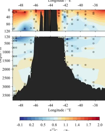
5.1.1 Interiorδ¹³C_DICdistribution

Our finalδ¹³C_DICresults are presented in Figs. 6–8. To first order,δ¹³CDICis highest in surface waters (shallower than ca. 40 m) taking values up to 2 ‰. Then,δ¹³CDICdecreases with depth to minima just below 0 ‰ at about 500 m, before increasing again to intermediate values of around 1 ‰ in deeper waters. This pattern is in general agreement with previous studies (Schmittner et al., 2013).

5.1.2 Cross-over analysis

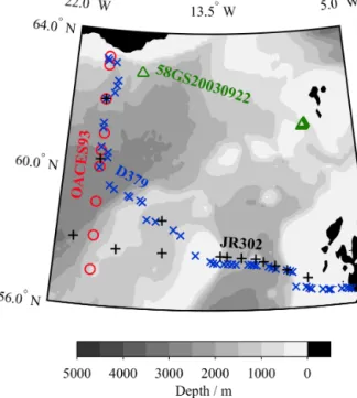
The cross-over analysis compared the results from this study with three nearby historical cruises: OACES93, 58GS20030922 and D379 (Table 2, Fig. 9). The mean δ¹³CDIC residual was significantly different from 0 for all of these cruises (p <0.01). Despite this, the mean (±SD) δ¹³CDICresiduals for OACES93 and D379 (−0.08±0.14 ‰ and +0.08±0.16 ‰ respectively) were no larger than our reported measurement precision of 0.08 ‰. Although the mean (±SD) residual for 58GS20030922 was greater (−0.19±0.16 ‰), it must firstly be considered that this de- pends on only three matching δ¹³C_DICmeasurements, and secondly that it is still within the range of the accuracy of 0.1–0.2 ‰ reported for its parent data set (Schmittner et al., 2013). These cruises and JR302 span a time interval of just over 20 years, so invasion of anthropogenic CO₂could have modified the δ¹³C_DICthrough the Suess effect (Keel- ing, 1979), potentially inhibiting the use of cross-over anal-

Figure 5.The V-PDB calibration. Mean values for each standard:

red square for MAB, green diamond for NA, and blue triangle for CA; results of individual measurements of standards shown as plusses in the same colours as the means. Thick black line shows the calibration curve (Eq. 5); dashed black lines enclose the range ofδ¹³C values for the seawater samples and RM.

ysis. However, in the deeper part of the water column in this region,δ¹³C_DIChas been observed to change at a rate of less than−0.01 ‰ yr⁻¹in recent decades (Humphreys et al., 2016). Thus the total change inδ¹³C_DICover the period between OACES93 (the earliest historical cruise) and JR302 should be no greater than the stated accuracy of the historical data set, and therefore our cross-over is valid. For future studies this will need to be reconsidered, as it might not hold true over longer timescales. We therefore conclude that any systematic bias between the results of this study and existing δ¹³CDICdata sets is negligible relative to the uncertainties of the measurements themselves.

5.2 Measurement uncertainty 5.2.1 Sample container types

In tests of duplicate samples collected in these two different container types, Humphreys et al. (2015a) were unable to find evidence of any systematic offset betweenδ¹³C_DIC measurements from the same two sample container types that were used in this study. Here, five pairs of sampling duplicates were collected with one sample in each container type. The mean±SD difference inδ¹³C_DICfor these duplicate pairs was−0.01±0.04 ‰, with the difference always calculated as theδ¹³C_DICvalue measured in the sample collected in a 50 mL vial subtracted from that collected in a

(7)

Table 2.Results of the cross-over analysis. Sources: OACES93 on R/VMalcolm Baldrige, carbon PIs F. Millero, R. Feely and P. Quay, data from Schmittner et al. (2013); 58GS20030922 on G. O.Sars, carbon PIs A. Olsen and T. Johannessen, data from Schmittner et al. (2013);

D379 on RRSDiscovery, carbon PI A. M. Griffiths, data from Humphreys et al. (2015a).

Cross-over Sampling Mean ofδ¹³C_DIC SD ofδ¹³C_DIC Number of

cruise date residuals/ ‰ residuals/ ‰ residuals

OACES93 Aug 1993 −0.08 0.14 19

58GS20030922 Oct 2003 −0.19 0.16 3

D379 Aug 2012 0.08 0.16 253

Figure 6. Zonal section of δ¹³C_DIC results from this study, from west to east across the subpolar North Atlantic Ocean (blue in Fig. 1). Coloured squares show actual sample locations and δ¹³C_DICvalues. Vertical dashed lines indicate locations of joints with edges of Figs. 7 and 8. Bathymetry data are from the GEBCO_2014 grid, version 20150318, http://www.gebco.net.

250 mL bottle. A one-samplet test could not reject the null hypothesis that this mean difference inδ¹³C_DICwas equal to 0 (p=0.63). We therefore conclude that the container type does not cause a systematic offset in the δ¹³C_DICmeasure- ment, in agreement with Humphreys et al. (2015a).

5.2.2 Seawater samples

The typical precision for seawater δ¹³C_DIC measurements is in the range from about 0.03 to 0.23 ‰ (Olsen et al.,

Figure 7. Zonal section of δ¹³C_DIC results from this study, from west to east near southern Greenland (orange in Fig. 1).

Coloured squares show actual sample locations andδ¹³C_DICval- ues. Bathymetry data are from the GEBCO_2014 grid, version 20150318, http://www.gebco.net.

2006; Quay et al., 2007; McNichol et al., 2010; Griffith et al., 2012), and we previously reported a value of 0.10 ‰ based on sampling duplicates (Humphreys et al., 2015a). In this study, we again determined the precision of the seawater sample measurements from both analytical and sampling duplicates. There were 341 analytical duplicate pairs, which had a mean absolute difference of 0.075 ‰ and therefore a 1σ precision of 0.067 ‰, and 36 sampling duplicate pairs, with a mean absolute difference of 0.090 ‰ and therefore a 1σ precision of 0.080 ‰. Although the latter is slightly greater, indicating that the sample collection and storage pro-

(8)

Figure 8.Meridional section ofδ¹³C_DICresults from this study, from south to north in the eastern subpolar North Atlantic Ocean (green in Fig. 1). Coloured squares show actual sample locations andδ¹³C_DICvalues. Bathymetry data are from the GEBCO_2014 grid, version 20150318, http://www.gebco.net.

cedures might have adversely affected the measurement precision, Levene’s test (Levene, 1960) carried out on the (non- absolute) duplicate differences could not reject the null hypothesis that the analytical and sampling precisions are in fact the same (p=0.33). We therefore report the higher value of 0.08 ‰ as the 1σ precision for this data set; it falls within the range of other studies of this kind. It is important to note that this value is based on consecutively analysed samples, and so might not reflect additional uncertainty en- gendered by samples being measured non-consecutively or in different analysis batches. However, it is shown in the following section that any such additional uncertainty was negligible.

5.2.3 Seawater reference material

Two “batches” of RM were measured in this study:

141 and 144 (http://cdiac.ornl.gov/oceans/Dickson_CRM/

batches.html). Each batch consists of multiple bottles of virtually identical seawater. Bottles from within each batch will henceforth be referred to as RM141 and RM144 respectively.

The RM are primarily intended for assessment of the accu-

Figure 9.Map of JR302 and historical sampling stations used in the cross-over analysis (Table 2). There were no stations suitable for cross-over analysis outside of the area shown on this map. Black plusses show JR302, blue crosses are D379, green triangles are 58GS20030922, and red circles are OACES93. Only historical stations within 150 km of a JR302 station were used, as described in Sect. 4.3.2.

racy of marine carbonate chemistry measurements, in particular DIC and TA (Dickson et al., 2003); they are sterilised and sealed in airtight bottles such that the DIC and TA are consistent in all RM bottles within each RM batch, and so these variables are stable and do not change on timescales of up to a few years. Although theδ¹³C_DICvalue is unknown for these RM, the nature of the preparation and storage process means that we can assume that it is also consistent within each RM batch (A. G. Dickson, personal communication, 18 June 2015), thus allowing us to assess the relative accuracy of ourδ¹³C_DICmeasurements between different analysis batches. Unpublished past measurements ofδ¹³CDICin similar RM (batches 17, 18 and 19) have supported this as- sumption, with theδ¹³CDICin multiple (i.e. 3–9) bottles from the same RM batch found to have a SD of about 0.01 ‰ (A.

G. Dickson, personal communication, 18 June 2015).

Typically, we made six measurements of each RM bottle, all within the same analysis batch. These were also spread throughout the analysis batch, and hence not consecutive (Fig. 2). The SD of these results for each bottle therefore represents a longer-term precision estimate than that which we get from the analytical duplicates, which were always analysed one immediately after the other. This approach therefore indicates the reproducibility of measurements carried out anywhere within a single analysis batch (rather than just

(9)

consecutively). The 1σ precision from the analytical duplicates was 0.067 ‰, while the average SD of the measurements within each RM bottle was slightly smaller (0.058 ‰).

This indicates that the position of samples within each analysis batch did not influence the δ¹³C_DICmeasurement; the relative accuracy of two consecutive measurements is no bet- ter than that between measurements from opposite ends of an analysis batch.

The next step is to verify that the difference in δ¹³C_DIC between different RM bottles of the same batch is negligible.

During analysis batch 13, we measured six different RM144 bottles, each up to six times (Table 3). The mean of the six measurements for each RM bottle was taken as its δ¹³CDIC

value. The SD of these six mean values was 0.028 ‰. Next, we compared this to measurements of different RM bottles across different analysis batches. One RM144 bottle was measured during each of analysis batches 1–12. The mean value was calculated for each analysis batch, and the SD of these 12 mean values was 0.056 ‰. Although larger than the SD for the six RM bottles within batch 13, this value is still smaller than the overall measurement precision based on samples within the same batch. In addition, we used Levene’s test (Levene, 1960) for the null hypothesis that the SD of the 6 RM bottles in analysis batch 13 was the same as the SD of the 12 RM bottles in analysis batches 1–12; the resulting p value of 0.14 was too great to confidently reject the null hypothesis, so we cannot be certain that there truly is greater variance between analysis batches than within them.

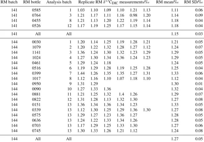
Our final δ¹³CDIC values are +1.15 ‰ for RM141 and +1.27 ‰ for RM144 (Table 3).

5.2.4 Calibration standards

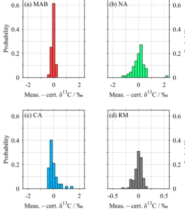
The precision of measurements of the calibration standards was greater (i.e. worse) than that of the samples and RM;

all calibrated MAB, NA and CA measurements had SDs of 0.13, 0.46, and 0.35 ‰ respectively, compared with about 0.08 ‰ for the RM (Fig. 10). We suggest that this is a result of the necessarily different practical treatment of the liquid seawater samples and RM compared with the powdered solid standards. The former were added to concentrated acid that had been overgassed with helium, while the latter were themselves overgassed prior to addition of dilute acid that may have contained some CO2. The blank correction should have corrected for the influence of this CO2, but there remained an unexplained relationship between peak area and rawδ¹³C for the standards even after its application (Fig. 4).

The poor precision for the standards might be associated with the very small quantities (0.1–1.1 mg) that were measured out into the Exetainer analysis vials, in contrast to the 1 mL of seawater sample or RM that was used each time – the former would be more susceptible to contamination. This result provides a strong incentive to develop seawater RM with a certifiedδ¹³C_DICvalue, which can be analysed following the

Figure 10. Histograms of offset of all standards and RM from their certified values (Table 1). Mean ± SD are (a) MAB, −0.03±0.13 ‰; (b) NA, +0.02±0.46 ‰; (c) CA,

−0.04±0.35 ‰; and (d) all RM, −0.01± 0.08 ‰. “Certified”

values for RM are our final values, 1.15 ‰ for RM141 and 1.27 ‰ for RM144 (Table 3). Note the increased horizontal resolution in (d).

exact same method as the samples during future studies of this kind.

5.3 Changes from our previous study

There were three main changes to the data processing from our previous study (Humphreys et al., 2015a): the peak area correction, which previously was carried out using a different relationship for the seawater samples and for each standard; the V-PDB calibration, which was previously carried out separately for each analysis batch; and the drift correction, which is absent in the current study.

5.3.1 Peak area (linearity) correction

The linearity correction in this study was different from that in our previous work (Humphreys et al., 2015a), because we did not find the same relationships between peak area and δ¹³C. This was due to hardware changes to the mass spectrometer in the intervening time between the studies. We therefore believe that the linearity correction used in each study was appropriate, and would recommend determining the best way to apply this correction on a case-by-case ba-

(10)

Table 3.Results of the RM measurements. The RM mean and standard deviation (SD) columns contain the mean and SD of the replicate values in each row, except for the rows marked “All”, which contain the mean and SD of all the RM mean values for each RM batch.

RM batch RM bottle Analysis batch Replicate RMδ¹³C_DICmeasurements/‰ RM mean/‰ RM SD/‰

141 0585 1 1.03 1.10 1.09 1.10 1.21 1.13 1.11 0.06

141 0764 3 1.21 1.17 1.11 1.16 0.98 1.20 1.14 0.09

141 0455 8 1.21 1.13 1.20 1.22 1.19 1.14 1.18 0.04

141 0526 12 1.17 1.19 1.25 1.17 1.15 1.14 1.18 0.04

141 All All 1.15 0.03

144 0030 1 1.20 1.14 1.25 1.19 1.28 1.21 1.21 0.05

144 1079 2 1.20 1.22 1.32 1.28 1.27 1.12 1.24 0.07

144 1141 3 1.36 1.24 1.30 1.32 1.23 1.29 1.29 0.05

144 1024 4 1.27 1.30 1.34 1.36 1.24 1.23 1.29 0.05

144 0461 5 1.29 1.24 1.18 1.24 0.05

144 0516 6 1.19 1.29 1.28 1.19 1.25 1.28 1.25 0.04

144 0399 7 1.44 1.26 1.35 1.35 1.27 1.31 1.33 0.06

144 1017 8 1.12 1.16 1.10 1.07 1.18 1.10 1.12 0.04

144 0950 9 1.31 1.29 1.30 0.01

144 0090 10 1.27 1.33 1.36 1.32 0.04

144 0881 11 1.21 1.25 1.32 1.4 1.26 1.29 0.07

144 0822 12 1.31 1.28 1.13 1.32 1.30 1.27 0.08

144 0151 13 1.36 1.34 1.36 1.34 1.23 1.33 0.05

144 0339 13 1.12 1.30 1.25 1.29 1.36 1.30 1.27 0.08

144 0575 13 1.29 1.27 1.23 1.36 1.27 1.28 0.05

144 0636 13 1.24 1.22 1.33 1.34 1.26 1.28 0.05

144 0703 13 1.17 1.29 1.25 1.33 1.30 1.27 0.06

144 0745 13 1.30 1.33 1.26 1.21 1.12 1.24 0.08

144 All All 1.27 0.05

sis for different data sets. Another result of these hardware changes was a reduction in the mean peak area for the seawater samples from about 35 mWb to about 20 mWb. There is no evidence of any adverse (or particularly beneficial) ef- fects on the quality of the results of either study as a result of these modifications.

5.3.2 The V-PDB calibration

The V-PDB calibration in this study was a single equation determined from all of the measurements of all of the calibration standards in every analysis batch, where previously we determined a separate equation for each batch (Humphreys et al., 2015a). This new approach delivered significantly bet- ter RM results between batches, as a result of the relatively high uncertainty in the measurements of the calibration standards; the apparent differences in calibration equations between analysis batches were in fact an artefact of these uncertainties. The consequence of this for our previous study is a decrease in precision, but it does not constitute a systematic error. If we apply a different calibration to each batch, as in our previous study, we find mean±SD across all analysis batches of the meanδ¹³C_DICof each RM within each batch for RM141 (4 RM bottles across 4 batches) and RM144 (18 RM bottles across 13 batches) of 1.19±0.08 and

1.30±0.11 ‰ respectively; by way of comparison, our new approach in this study yields 1.15±0.03 and 1.26±0.05 ‰ respectively. To determine the significance of these apparent differences, we took the mean RM141 and RM144 results for each analysis batch and used them to test two different null hypotheses, separately for each RM and calibration method.

Firstly, we used Welch’s unequal variances t test (Welch, 1947) for the null hypothesis that the meanδ¹³CDICacross all batches was the same regardless of the V-PDB calibration method. For both RM141 and RM144, the null hypothesis could not be rejected at the 5 % significance level, with p values of 0.47 and 0.28 respectively. Secondly, we used Levene’s test (Levene, 1960) for the null hypothesis that the variance of these batch mean results was the same regardless of the V-PDB calibration method. For both RM141 and RM144, the null hypothesis was rejected at the 5 % significance level, with p values of 0.01 and 0.03 respectively.

Thus we conclude that the change to the V-PDB calibration method – using a single equation across all analysis batches, instead of a separate one for each – results in an improvement in the precision of results from different analysis batches (i.e.

reduced SD), and that it does not cause a systematic bias in these results (i.e. no change in the mean).

(11)

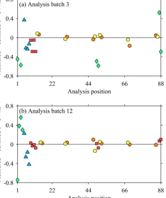
Figure 11.Examples of results of standards and RM within batches (a)3 and(b)12. Red squares for MAB, green diamonds for NA, blue triangles for CA, orange circles for RM141, and yellow circles for RM144.

This result cannot necessarily be applied to recalibrate the results of our previous study, as no RM measurements were carried out then. In this study, all measurements were carried out on consecutive days over a 5-week period. However, in the previous study, there were gaps of several weeks between some analysis batches, and there is no way to objectively assess the consistency of the calibration over these breaks retrospectively. Therefore, although the uncertainty estimate for the previous study was probably too generous (i.e. the reported uncertainty was lower than it should have been) and should be approximately doubled, there is no evidence of a systematic bias.

Additionally, the form of the equation used to carry out the V-PDB calibration (Eq. 5) is a second-order polynomial in this study, which differs from the circle used by Humphreys et al. (2015a). This change makes virtually no difference to the finalδ¹³C_DICresults, but it provides a calibration equation that only gives one possible corrected value for each input δ¹³C. The calibration equation used in this study is also much easier to interpret, with coefficients directly cor- responding to the curvature (c), stretch (s) and translational offset (f) of the curve.

5.3.3 Drift correction

No drift correction was performed during this study, while Humphreys et al. (2015a) used the measurements of pairs

standards at the middle and end of each analysis batch to cor- rect for instrumental drift. However, the RM measurements spaced throughout each analysis batch in the present study indicated that no drift correction was required, sometimes in disagreement with the calibration standards (Fig. 11). We suggest that this apparent conflict is again a result of the significantly greater uncertainty in individual measurements of the calibration standards relative to those of seawater samples and RM.

As for the V-PDB calibration, this difference does not cause an important systematic offset to the results from our previous study, but rather an increase in the variance. To support this claim, we applied a drift correction following Humphreys et al. (2015a) to our RM144 results in analysis batches 1–8 and 10–12. Analysis batches 9 and 13 were excluded due to the lack of RM data and the different arrangement of RM respectively (Fig. 2). The mean±SD of all individual RM144 measurements (i.e. up to 6 per RM bottle) was 1.26±0.08 ‰ with no drift correction, but 1.22±0.17 ‰ when a drift correction was applied. We used Levene’s test (Levene, 1960) to confidently reject the null hypothesis that the SDs were equal with and without the drift correction (p=0.0001), and thus the decline in precision caused by applying the drift correction was significant. We also used Welch’s unequal variancest test (Welch, 1947) for the null hypothesis that the mean value of these RM144 measurements were the same with and without drift correction; although the null hypothesis could be tentatively rejected at the 5 % significance level (p=0.048) the actual magnitude of the difference in the mean values (ca. 0.04 ‰) is smaller than the measurement precision of either study, and can therefore be considered negligible.

However, for the same reasons as given regarding the V- PDB calibration, it would not be appropriate to recommend retrospective changes to the results of our previous study in the absence of any RM measurements therein.

6 Conclusions

We successfully measuredδ¹³C_DICin 341 samples collected from June to July 2014 during RRSJames Clark Rosscruise JR302 in the subpolar North Atlantic Ocean. The δ¹³CDIC

values were in the range from−0.07 to+1.95 ‰ relative to V-PDB and had a 1σ uncertainty of 0.08 ‰. Our results are internally consistent, with no systematic offsets between or within analysis batches, and a cross-over analysis revealed no systematic bias relative to nearby historical data in deep waters. We have also establishedδ¹³C_DICvalues for batches 141 (+1.15 ‰) and 144 (+1.27 ‰) of seawater RM obtained from A. G. Dickson (Scripps Institute of Oceanography, USA), and demonstrated that RM bottles within the same batch have consistentδ¹³C_DICvalues. These RMs greatly en- hanced our ability to quantitatively assess and improve our data processing approach, and lead us to conclude that the de-

(12)

velopment of an internationally available seawater RM with a certifiedδ¹³C_DICvalue would be a valuable boon to future measurements of this kind.

7 Data set availability

Theδ¹³CDICmeasurements described in this study are pub- licly available, free of charge, from the British Oceano- graphic Data Centre, with doi:10.5285/22235f1a-b7f3-687f- e053-6c86abc0c8a6 (Humphreys et al., 2015b). The data will also be submitted to the Carbon Dioxide Information Analysis Centre (CDIAC, Oak Ridge National Laboratory, USA) along with other carbonate chemistry and macronutri- ent metadata from cruise JR302 once those become available.

Author contributions. E. Tynan determined the sampling strat- egy, and E. Tynan, A. M. Griffiths, C. H. Fry and R. Garley collected the samples. F. M. Greatrix, A. McDonald and M. P. Humphreys carried out the measurements and data processing. M. P. Humphreys wrote the manuscript with contributions from all co-authors.

Acknowledgements. We acknowledge funding from the Natural Environment Research Council (UK) for the carbon isotope analyses (IP-1449-0514) and the RAGNARoCC award to the University of Southampton for ship time (NE-K002546-1). We are grateful to the officers, crew and scientists on board RRS James Clark Rossfor their hard work and support during cruise JR302.

We thank Matt Donnelly (BODC) for handling the archiving of our data.

Edited by: D. Carlson

References

Achterberg, E. P.: Grand challenges in marine biogeochemistry, Front. Mar. Sci., 1, 7, doi:10.3389/fmars.2014.00007, 2014.

Becker, M., Andersen, N., Erlenkeuser, H., Humphreys, Matthew.

P., Tanhua, T., and Körtzinger, A.: An Internally Consistent Dataset ofδ¹³C-DIC in the North Atlantic Ocean – NAC13v1, Earth Syst. Sci. Data Discuss., doi:10.5194/essd-2016-7, in review, 2016.

Brewer, P. G.: Direct observation of the oceanic CO₂increase, Geo- phys. Res. Lett., 5, 997–1000, doi:10.1029/GL005i012p00997, 1978.

Caldeira, K. and Wickett, M. E.: Anthropogenic carbon and ocean pH, Nature, 425, 365–365, doi:10.1038/425365a, 2003.

Chen, G.-T. and Millero, F. J.: Gradual increase of oceanic CO₂, Nature, 277, 205–206, doi:10.1038/277205a0, 1979.

Coplen, T. B.: Reporting of stable hydrogen, carbon, and oxygen isotopic abundances, Geothermics, 24, 707–712, doi:10.1016/0375-6505(95)00024-0, 1995.

Dickson, A. G., Afghan, J. D., and Anderson, G. C.: Reference ma- terials for oceanic CO₂analysis: a method for the certification of total alkalinity, Mar. Chem., 80, 185–197, doi:10.1016/S0304- 4203(02)00133-0, 2003.

Dickson, A. G., Sabine, C. L., and Christian, J. R.: Guide to best practices for ocean CO₂measurements, PICES Special Publica- tion 3, 191 pp., 2007.

Doney, S. C., Fabry, V. J., Feely, R. A., and Kleypas, J. A.: Ocean Acidification: The Other CO₂ Prob- lem, Annual Review of Marine Science, 1, 169–192, doi:10.1146/annurev.marine.010908.163834, 2009.

Friis, K., Körtzinger, A., Pätsch, J., and Wallace, D. W. R.:

On the temporal increase of anthropogenic CO₂ in the subpolar North Atlantic, Deep-Sea Res. Pt. I, 52, 681–698, doi:10.1016/j.dsr.2004.11.017, 2005.

Gaylord, B., Kroeker, K. J., Sunday, J. M., Anderson, K. M., Barry, J. P., Brown, N. E., Connell, S. D., Dupont, S., Fabricius, K. E., Hall-Spencer, J. M., Klinger, T., Milazzo, M., Munday, P. L., Russell, B. D., Sanford, E., Schreiber, S. J., Thiyagarajan, V., Vaughan, M. L. H., Widdicombe, S., and Harley, C. D. G.: Ocean acidification through the lens of ecological theory, Ecology, 96, 3–15, doi:10.1890/14-0802.1, 2015.

Griffith, D. R., McNichol, A. P., Xu, L., McLaughlin, F. A., Mac- donald, R. W., Brown, K. A., and Eglinton, T. I.: Carbon dy- namics in the western Arctic Ocean: insights from full-depth carbon isotope profiles of DIC, DOC, and POC, Biogeosciences, 9, 1217–1224, doi:10.5194/bg-9-1217-2012, 2012.

Gruber, N., Sarmiento, J. L., and Stocker, T. F.: An improved method for detecting anthropogenic CO₂in the oceans, Global Biogeochem. Cy., 10, 809–837, doi:10.1029/96GB01608, 1996.

Hall, T. M., Haine, T. W. N., and Waugh, D. W.: In- ferring the concentration of anthropogenic carbon in the ocean from tracers, Global Biogeochem. Cy., 16, 1131, doi:10.1029/2001GB001835, 2002.

Holliday, N. P. and Cunningham, S.: The Extended Ellett Line:

Discoveries from 65 years of marine observations west of the UK, Oceanography, 26, 156–163, doi:10.5670/oceanog.2013.17, 2013.

Humphreys, M. P.: Cross-over analysis of hydrographic variables: XOVER v1.0, Ocean and Earth Science, University of Southampton, UK, 8 pp., doi:10.13140/RG.2.1.1629.0405, 2015.

Humphreys, M. P., Achterberg, E. P., Griffiths, A. M., McDonald, A., and Boyce, A. J.: Ellett Line measurements of stable isotope composition of dissolved inorganic carbon in the Northeastern Atlantic and Nordic Seas during summer 2012, British Oceano- graphic Data Centre, Natural Environment Research Council, UK, doi:10/xph, 2014a.

Humphreys, M. P., Achterberg, E. P., Griffiths, A. M., McDonald, A., and Boyce, A. J.: UKOA measurements of the stable isotope composition of dissolved inorganic carbon in the Northeastern Atlantic and Nordic Seas during summer 2012, British Oceano- graphic Data Centre, Natural Environment Research Council, UK, doi:10/xpj, 2014b.

Humphreys, M. P., Achterberg, E. P., Griffiths, A. M., McDonald, A., and Boyce, A. J.: Measurements of the stable carbon isotope composition of dissolved inorganic carbon in the northeastern Atlantic and Nordic Seas during summer 2012, Earth Syst. Sci.

Data, 7, 127–135, doi:10.5194/essd-7-127-2015, 2015a.

Humphreys, M. P., Greatrix, F. M., Tynan, E., Griffiths, A. M., Fry, C. H., Garley, R., Achterberg, E. P., McDonald, A., and Boyce, A. J.: Stable carbon isotopes of dissolved inorganic carbon for RRSJames Clark Ross cruise JR302 in the subpolar North Atlantic Ocean from June to July 2014, British Oceano-

(13)

graphic Data Centre, Natural Environment Research Coun- cil, UK, doi:10.5285/22235f1a-b7f3-687f-e053-6c86abc0c8a6, 2015b.

Humphreys, M. P., Griffiths, A. M., Achterberg, E. P., Holliday, N.

P., Rérolle, V. M. C., Menzel Barraqueta, J.-L., Couldrey, M. P., Oliver, K. I. C., Hartman, S. E., Esposito, M., and Boyce, A.

J.: Multidecadal accumulation of anthropogenic and remineral- ized dissolved inorganic carbon along the Extended Ellett Line in the northeast Atlantic Ocean, Global Biogeochem. Cy., 30, 2015GB005246, doi:10.1002/2015GB005246, 2016.

Keeling, C. D.: The Suess effect:¹³Carbon-¹⁴Carbon interrelations, Environ. Int., 2, 229–300, doi:10.1016/0160-4120(79)90005-9, 1979.

Khatiwala, S., Primeau, F., and Hall, T.: Reconstruction of the his- tory of anthropogenic CO₂concentrations in the ocean, Nature, 462, 346–349, doi:10.1038/nature08526, 2009.

Khatiwala, S., Tanhua, T., Mikaloff Fletcher, S., Gerber, M., Doney, S. C., Graven, H. D., Gruber, N., McKinley, G. A., Murata, A., Ríos, A. F., and Sabine, C. L.: Global ocean storage of anthropogenic carbon, Biogeosciences, 10, 2169–2191, doi:10.5194/bg-10-2169-2013, 2013.

King, B. A. and Holliday, N. P.: JR302 Cruise Report, The 2014 RAGNARoCC, OSNAP and Extended Ellett Line cruise, Na- tional Oceanography Centre, Southampton, UK, 76 pp., 2015.

Körtzinger, A., Quay, P. D., and Sonnerup, R. E.: Relationship between anthropogenic CO₂ and the ¹³C Suess effect in the North Atlantic Ocean, Global Biogeochem. Cy., 17, 5-1–5-20, doi:10.1029/2001GB001427, 2003.

Lauvset, S. K. and Tanhua, T.: A toolbox for secondary quality control on ocean chemistry and hydrographic data, Limnol.

Oceanogr.-Meth., doi:10.1002/lom3.10050, 2015.

Le Quéré, C., Raupach, M. R., Canadell, J. G., Marland, G., Bopp, L., Ciais, P., Conway, T. J., Doney, S. C., Feely, R. A., Foster, P., Friedlingstein, P., Gurney, K., Houghton, R. A., House, J. I., Huntingford, C., Levy, P. E., Lomas, M. R., Majkut, J., Metzl, N., Ometto, J. P., Peters, G. P., Prentice, I. C., Randerson, J. T., Running, S. W., Sarmiento, J. L., Schuster, U., Sitch, S., Taka- hashi, T., Viovy, N., van der Werf, G. R., and Woodward, F. I.:

Trends in the sources and sinks of carbon dioxide, Nat. Geosci., 2, 831–836, doi:10.1038/ngeo689, 2009.

Levene, H.: Robust tests for equality of variances, in Contribu- tions to Probability and Statistics: Essays in Honor of Harold Hotelling, 278–292, Stanford University Press, USA, 1960.

McNichol, A., Quay, P. D., Gagnon, A. R., and Burton, J. R.: Col- lection and measurement of carbon isotopes in seawater DIC, in The GO-SHIP Repeat Hydrography Manual: A Collection of Ex- pert Reports and Guidelines, IOCCP Report No. 14, ICPO Pub- lication Series No. 134, Version 1, 2010.

Olsen, A. and Ninnemann, U.: Large δ¹³C Gradients in the Preindustrial North Atlantic Revealed, Science, 330, 658–659, doi:10.1126/science.1193769, 2010.

Olsen, A., Omar, A. M., Bellerby, R. G. J., Johannessen, T., Ninne- mann, U., Brown, K. R., Olsson, K. A., Olafsson, J., Nondal, G., Kivimäe, C., Kringstad, S., Neill, C., and Olafsdottir, S.: Mag- nitude and origin of the anthropogenic CO₂ increase and¹³C Suess effect in the Nordic seas since 1981, Global Biogeochem.

Cy., 20, GB3027, doi:10.1029/2005GB002669, 2006.

Quay, P., Sonnerup, R., Westby, T., Stutsman, J., and McNichol, A.: Changes in the ¹³C/¹²C of dissolved inorganic carbon in

the ocean as a tracer of anthropogenic CO₂uptake, Global Bio- geochem. Cy., 17, GB1004, doi:10.1029/2001GB001817, 2003.

Quay, P. D., Tilbrook, B., and Wong, C. S.: Oceanic Uptake of Fossil Fuel CO₂: Carbon-13 Evidence, Science, 256, 74–79, doi:10.1126/science.256.5053.74, 1992.

Quay, P. D., Sonnerup, R., Stutsman, J., Maurer, J., Körtzinger, A., Padin, X. A., and Robinson, C.: Anthropogenic CO₂accumulation rates in the North Atlantic Ocean from changes in the 13C/¹²C of dissolved inorganic carbon, Global Biogeochem. Cy., 21, GB1009, doi:10.1029/2006GB002761, 2007.

Rubino, M., Etheridge, D. M., Trudinger, C. M., Allison, C. E., Bat- tle, M. O., Langenfelds, R. L., Steele, L. P., Curran, M., Bender, M., White, J. W. C., Jenk, T. M., Blunier, T., and Francey, R. J.:

A revised 1000? year atmosphericδ¹³C-CO₂record from Law Dome and South Pole, Antarctica, J. Geophys. Res. Atmos., 118, 8482–8499, doi:10.1002/jgrd.50668, 2013.

Sabine, C. L. and Tanhua, T.: Estimation of Anthropogenic CO₂ Inventories in the Ocean, Annual Review of Marine Science, 2, 175–198, doi:10.1146/annurev-marine-120308-080947, 2010.

Sabine, C. L., Feely, R. A., Gruber, N., Key, R. M., Lee, K., Bullis- ter, J. L., Wanninkhof, R., Wong, C. S., Wallace, D. W. R., Tilbrook, B., Millero, F. J., Peng, T.-H., Kozyr, A., Ono, T., and Rios, A. F.: The Oceanic Sink for Anthropogenic CO₂, Science, 305, 367–371, doi:10.1126/science.1097403, 2004.

Schmittner, A., Gruber, N., Mix, A. C., Key, R. M., Tagliabue, A., and Westberry, T. K.: Biology and air–sea gas exchange controls on the distribution of carbon isotope ratios (δ¹³C) in the ocean, Biogeosciences, 10, 5793–5816, doi:10.5194/bg-10-5793-2013, 2013.

Sonnerup, R. E. and Quay, P. D.: ¹³C constraints on ocean carbon cycle models, Global Biogeochem. Cy., 26, GB2014, doi:10.1029/2010GB003980, 2012.

Sonnerup, R. E., Quay, P. D., McNichol, A. P., Bullister, J.

L., Westby, T. A., and Anderson, H. L.: Reconstructing the oceanic¹³C Suess Effect, Global Biogeochem. Cy., 13, 857–872, doi:10.1029/1999GB900027, 1999.

Sonnerup, R. E., McNichol, A. P., Quay, P. D., Gammon, R. H., Bullister, J. L., Sabine, C. L., and Slater, R. D.: Anthropogenic δ¹³C changes in the North Pacific Ocean reconstructed using a multiparameter mixing approach (MIX), Tellus B, 59, 303–317, doi:10.1111/j.1600-0889.2007.00250.x, 2007.

Tanhua, T., Körtzinger, A., Friis, K., Waugh, D. W., and Wallace, D.

W. R.: An estimate of anthropogenic CO₂inventory from decadal changes in oceanic carbon content, Proc. Natl. Acad. Sci. USA, 104, 3037–3042, doi:10.1073/pnas.0606574104, 2007.

Thompson, M. and Howarth, R. J.: The rapid estimation and control of precision by duplicate determinations, Analyst, 98, 153–160, doi:10.1039/AN9739800153, 1973.

Waugh, D. W., Hall, T. M., McNeil, B. I., Key, R., and Matear, R. J.: Anthropogenic CO₂ in the oceans estimated using tran- sit time distributions, Tellus B, 58, 376–389, doi:10.1111/j.1600- 0889.2006.00222.x, 2006.

Welch, B. L.: The Generalization of Student’s Problem When Sev- eral Different Population Variances Are Involved, Biometrika, 34, 28–35, doi:10.1093/biomet/34.1-2.28, 1947.