A global monthly climatology of oceanic total dissolved inorganic carbon: a neural network approach

(1)

https://doi.org/10.5194/essd-12-1725-2020

A global monthly climatology of oceanic total dissolved inorganic carbon: a neural network approach

Daniel Broullón¹, Fiz F. Pérez¹, Antón Velo¹, Mario Hoppema², Are Olsen³, Taro Takahashi^4,, Robert M. Key⁵, Toste Tanhua⁶, J. Magdalena Santana-Casiano⁷, and Alex Kozyr⁸

1Instituto de Investigaciones Marinas, CSIC, Eduardo Cabello 6, 36208 Vigo, Spain

2Alfred Wegener Institute Helmholtz Centre for Polar and Marine Research, Postfach 120161, 27515 Bremerhaven, Germany

3Geophysical Institute, University of Bergen and Bjerknes Centre for Climte Research, Allégaten 70, 5007 Bergen, Norway

4Lamont–Doherty Earth Observatory of Columbia University, Palisades, NY 10964, USA

5Atmospheric and Oceanic Sciences, Princeton University, 300 Forrestal Road, Sayre Hall, Princeton, NJ 08544, USA

6GEOMAR Helmholtz Centre for Ocean Research Kiel, Düsternbrooker Weg 20, 24105 Kiel, Germany

7Instituto de Oceanografía y Cambio Global, IOCAG, Universidad de Las Palmas de Gran Canaria, Las Palmas de Gran Canaria, Spain

8NOAA National Centers for Environmental Information, 1315 East-West Hwy Silver Spring, MD 20910, USA

deceased

Correspondence:Daniel Broullón (dbroullon@iim.csic.es) Received: 14 February 2020 – Discussion started: 11 March 2020 Revised: 18 June 2020 – Accepted: 2 July 2020 – Published: 5 August 2020

Abstract. Anthropogenic emissions of CO₂to the atmosphere have modified the carbon cycle for more than 2 centuries. As the ocean stores most of the carbon on our planet, there is an important task in unraveling the natural and anthropogenic processes that drive the carbon cycle at different spatial and temporal scales. We contribute to this by designing a global monthly climatology of total dissolved inorganic carbon (TCO₂), which offers a robust basis in carbon cycle modeling but also for other studies related to this cycle. A feedforward neural network (dubbed NNGv2LDEO) was configured to extract from the Global Ocean Data Analysis Project version 2.2019 (GLODAPv2.2019) and the Lamont–Doherty Earth Observatory (LDEO) datasets the relations between TCO₂ and a set of variables related to the former’s variability. The global root mean square error (RMSE) of mapping TCO2 is relatively low for the two datasets (GLODAPv2.2019: 7.2 µmol kg⁻¹; LDEO:

11.4 µmol kg⁻¹) and also for independent data, suggesting that the network does not overfit possible errors in data. The ability of NNGv2LDEO to capture the monthly variability of TCO2 was testified through the good reproduction of the seasonal cycle in 10 time series stations spread over different regions of the ocean (RMSE: 3.6 to 13.2 µmol kg⁻¹). The climatology was obtained by passing through NNGv2LDEO the monthly climatological fields of temperature, salinity, and oxygen from the World Ocean Atlas 2013 and phosphate, nitrate, and silicate computed from a neural network fed with the previous fields. The resolution is 1^◦×1^◦in the horizontal, 102 depth levels (0–5500 m), and monthly (0–1500 m) to annual (1550–5500 m) temporal resolution, and it is centered around the year 1995. The uncertainty of the climatology is low when compared with climatological values derived from measured TCO₂in the largest time series stations. Furthermore, a computed climatology of partial pressure of CO₂(pCO₂) from a previous climatology of total alkalinity and the present one of TCO₂supports the robustness of this product through the good correlation with a widely usedpCO₂climatology (Landschützer et al., 2017). Our TCO₂climatology is distributed through the data repository of the Spanish National Research Council (CSIC; https://doi.org/10.20350/digitalCSIC/10551, Broullón et al., 2020).

(2)

1 Introduction

The ocean is the major carbon reservoir of the Earth. Most of this carbon occurs as dissolved inorganic carbon (TCO2, also known as DIC or CT; Ciais et al., 2013; Tanhua et al., 2013).

Three species make up TCO2: dissolved CO2(generally considered to be the sum of the dissolved CO₂itself, CO₂(aq), and carbonic acid, H₂CO₃), bicarbonate ion (HCO⁻₃), and carbonate ion (CO²⁻₃ ). The relative concentrations of these species with respect to each other determine the seawater pH (Zeebe and Wolf-Gladrow, 2001). The seawater CO₂chemistry system can be represented as a set of chemical equilib- ria reactions that describe the speciation of the various ions of TCO2as follows:

CO₂(g)CO₂(aq) CO2(aq)+H2OH2CO3

H₂CO₃H⁺+HCO⁻₃ HCO⁻₃ H⁺+CO²⁻₃ .

Since the Industrial Revolution, the concentration of TCO₂in the global ocean has increased, generally to a certain depth level (depending on the particular processes in each ocean area) due to the entry of CO₂into the seawater from the atmosphere (Sarmiento and Gruber, 2002; Doney et al., 2009;

Vázquez-Rodríguez et al., 2009; Bates et al., 2012; Sallée et al., 2012; Khatiwala et al., 2013). The uptake is driven by the increasing partial pressure of CO2(pCO2) in the atmosphere relative to the ocean, generated by the anthropogenic emissions of CO₂ that cause an annual net flux of this gas into the ocean (Le Quéré et al., 2018). Accompanying the change in TCO₂, the pH and carbonate ion concentration have been declining because of the anthropogenic process previously mentioned, these changes being reflected in the proportions of the chemical species of TCO₂ (Kleypas and Langdon, 2000; Orr et al., 2005). These changes in seawater chemistry framed in the ocean acidification process can negatively influence various processes involving marine or- ganisms such as calcification, growth, and survival (Orr et al., 2005; Fabry et al., 2008; Hendriks et al., 2010; Hoegh- Guldberg and Bruno, 2010; Kroeker et al., 2013).

In addition to the secular trends driven by the uptake of anthropogenic CO2, ocean TCO2varies both temporally and spatially as a consequence of several natural processes. This variability may reach values of 15 % of the mean TCO₂value in the ocean (Lee et al., 2000). The processes that increase TCO₂are net flux of CO₂from the atmosphere to the ocean, organic matter remineralization, and the dissolution of cal- cium carbonate (CaCO₃). The processes that reduce TCO₂ are net flux of CO₂from the ocean to the atmosphere, pri- mary production, and calcification. Advection and mixing also influence the variability of TCO₂ in these two ways (Sabine et al., 2002). In the surface ocean, the main vari-

ables influencing the variability of TCO₂ are temperature and salinity (Weiss et al., 1982; Lee et al., 2000; Wu et al., 2019), through the modification of the solubility of CO₂, af- fecting the seawaterpCO2(which is almost instantaneous) and thus the air–sea CO2flux, which eventually drives the change in TCO2 over time. Nutrients and oxygen can also reflect the processes that modify the concentration of TCO2

through their consumption and release, like during the cy- cling of organic matter (Körtzinger et al., 2001; Bauer et al., 2013). From products generated with measured data (Key et al., 2004; Takahashi et al., 2014; Lauvset et al., 2016) and in modeling studies (e.g., Doi et al., 2015), it is known that the global surface distribution of TCO₂follows a zonal gradient:

there is a reduction in its concentration from the poles to the Equator, reflecting the processes that control its variability.

Key et al. (2004) emphasize that this distribution is associated with the distribution pattern of nutrients. Recently, Wu et al. (2019) found that the distribution of surface-salinity- normalized TCO2(nDIC) has two main drivers: temperature and upwelling. At depth, the variation shown in almost any measured profile of TCO2mainly reflects the remineralization of organic matter and, to a lesser extent, the dissolution of CaCO₃(Millero, 2007), resulting in an increase in TCO₂ from the surface to intermediate depths.

Understanding the distribution and variability of TCO₂ in the ocean and its secular trends driven by anthropogenic carbon uptake is needed to assess the magnitude and possible impacts of ocean acidification. It is also necessary for the evaluation of numerical models that include the carbon cycle and their estimates of past, current, and future ocean carbon cycle behavior (e.g., Yool et al., 2013; Au- mont et al., 2015; Butenschön et al., 2016; Le Quéré et al., 2016;) Goris et al., 2018). Seasonality of TCO2and the horizontal and vertical variability underscore the necessity to design a climatology with both monthly and spatial resolu- tions according to the processes that influence this variable on a global scale. The existing climatologies of TCO2 do not include all these characteristics collected together. Key et al. (2004) and Lauvset et al. (2016) built an annual climatology at 33 depth levels using interpolation techniques with data from the Global Ocean Data Analysis Project version 1 (GLODAPv1; Key et al., 2004) and version 2 (GLO- DAPv2; Key et al., 2015; Olsen et al., 2016), respectively.

Takahashi et al. (2014) published a monthly climatology for the surface ocean computed from climatologies ofpCO₂and total alkalinity (A_T). Other studies used the covariability between TCO₂and other more commonly measured variables discussed above for mapping and gap-filling via empirical regressions and neural networks. Lee et al. (2000) used temperature and nitrate to compute surface nDIC with an area- weighted error of±7 µmol kg⁻¹. Sauzède et al. (2017) and Bittig et al. (2018) trained neural networks with GLODAPv2 data to compute TCO₂over the depth range 0–8000 m with

(3)

an accuracy of±9 and±7.1 µmol kg⁻¹, respectively. The input variables used in those studies were location, pressure, temperature, salinity, dissolved oxygen, and time.

In the present study, we introduce the use of neural networks for going one step further in the design of a climatology. We have generated a climatology of TCO₂with a resolution consistent with that of the climatology ofA_Tof Broul- lón et al. (2019): horizontal resolution of 1^◦×1^◦, 102 depth levels between 0 and 5500 m, and a monthly (0–1500 m) and annual (1550–5500 m) temporal resolution. The availability of global databases containing variables of the seawater CO₂ system with more and more data – e.g., GLODAPv2.2019;

the Lamont–Doherty Earth Observatory (LDEO) database (Takahashi et al., 2017); the Surface Ocean CO2Atlas (SO- CAT; Bakker et al., 2016) – and the great ability of the neural networks to interpolate as shown in other climatological studies about CO₂system variables (Landschützer et al., 2014; Broullón et al., 2019) show the appropriateness of this approach for generating a global monthly climatology cover- ing more than the surface ocean.

2 Methodology

2.1 Neural network design

A feedforward neural network was configured to compute TCO2 in the global ocean and to create a global climatology based on the good results previously obtained with this method in similar studies (e.g., Broullón et al., 2019). Briefly, a neural network of this type (Fig. S1a in the Supplement) is used to extract relationships between a set of input variables and a target one through a training process. At this stage, the inputs are passed through different parallel layers composed of a tunable number of neurons to reach values as closest as possible to the target ones (Fig. S1a). Initially, all inputs en- ter each neuron of the first layer, where they are multiplied by different weights depending on the neuron they go to. Inside the neurons (Fig. S1b), the results of the previous operation are summed, and a bias is added. The obtained value inside each neuron is passed through an activation function, which yields an output. The outputs of each neuron in each layer go to the following layer undergoing the same process described to this point. In the last layer, which is composed of one neuron, a unique value for the target variable is calculated for each pair consisting of inputs and a target. This value is compared to the desired one, and the difference between both values is backpropagated through the entire network in order to adjust the weights and biases and to start the processes again and reach an accurate output value after multiple iterations.

A complete description of the most common algorithms used to backpropagate and minimize the errors can be found in Rumelhart et al. (1986), Levenberg (1944), and Marquardt (1963).

The method used here is equivalent to that fully described by Broullón et al. (2019) forA_T. In addition to the target vari-

able (TCO2instead ofAT), the main changes in the present study compared to that of Broullón et al. (2019) are the inclusion of the input variable “year”, accounting for the anthropogenic increase in the TCO₂pool, and the use of thepCO₂ database from the LDEO (Takahashi et al., 2017) in addition to the extended GLODAPv2.2019 (Olsen et al., 2019) to enable more robust TCO₂estimates in the surface ocean.

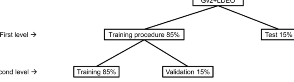
Similar to Broullón et al. (2019), the neural networks were trained using the Levenberg–Marquardt method (Levenberg, 1944; Marquardt, 1963) through the trainlm function (de- tailed in Beale et al., 2018) in MATLAB. The splitting of the database used in the present study (see Sect. 2.2) into the sets needed for training and testing the network is depicted in Fig. 1. The data were randomly associated with each dataset to capture (training) and evaluate (test) all possible variability. The input variables are temperature, salinity, phosphate, nitrate, silicate, oxygen, sample position, and year (Fig. S1a).

The number of neurons tested in the unique hidden layer to find the best neural network was 16, 32, 64, 128, and 256.

Ten networks were trained for each number of neurons. The criteria for selecting the final number of neurons are based on a trade-off between the root mean square error (RMSE;

between the measured TCO₂and that estimated by the neural network) on the one hand and the generalization of the network (to prevent overfitting, maintaining a similar error in the training and in the test sets) on the other hand. Further- more, an additional criterion based on the influence of each input variable on the TCO2 extracted with the connection weight approach (Olden and Jackson, 2002) was followed to ensure that biogeochemical input variables have a larger influence on the TCO2estimates than the input variables related to sample position for selecting a proper network. The influence of each input variable on the computed TCO₂was obtained from Eq. (1):

C_i=

H

X

k=1

w_ik·w_k, (1)

whereC_iis the relative importance of the input variablei,H the number of neurons in the hidden layer,w_ikthe weight of the connection between the variableiand the neuronkof the hidden layer, andwk the weight of the connection between the neuronkof the hidden layer and output layer.

2.2 Data

We included the LDEO database version 2016 (Taka- hashi et al., 2017; https://www.nodc.noaa.gov/ocads/oceans/

LDEO_Underway_Database, last access: 13 November 2017) because it contains significantly more data in the surface layer than GLODAPv2.2019. Since the higher variability in the surface layer may lead to high errors in modeling variables of the seawater CO₂system (e.g., Carter et al., 2018; Bittig et al., 2018; Broullón et al., 2019), including the LDEO database should force the network to reach a more

(4)

Figure 1.Division of the complete database in the datasets needed to train the neural network. The percentages in each level are relative to the number of data in the previous one. Data in the datasets of the first level are always the same for each network. Data in the sets of the second level are randomly associated with each set for each network to find the best network weights because of the different starting points in the error weight space of the training process (see also Broullón et al., 2019).

robust fit. The idea is that these additional data probably have more different relationships between input variables and TCO₂to help the neural network to adequately capture spatiotemporal variability. The pCO₂, temperature, and salinity data from the LDEO were monthly averaged for each year in a 1^◦×1^◦ grid. The points where the standard devi- ation (SD) of the averaged pCO₂, temperature, and salinity were greater than±20 µatm, 1.5^◦C, and 0.5, respectively, were discarded since the objective is to capture the monthly variability, and therefore an extremely high submonthly variability could lead to errors. To obtain TCO₂values from the LDEO data, an additional variable of the CO2system is necessary, for which we take AT computed using the neural network NNGv2 of Broullón et al. (2019). The input variables required by NNGv2 were obtained from (1) temperature and salinity from the LDEO; (2) filtered oxygen from the World Ocean Atlas version 2013 (WOA13; see Broullón et al., 2019); and (3) phosphate, nitrate, and silicate computed with CANYON-B (Bittig et al., 2018) using the previous variables as inputs. Finally, TCO₂was calculated from thisA_Tand the averagedpCO₂using the MATLAB version of the CO_2SYS program (van Heuven et al., 2011); we used the dissociation constants of Mehrbach et al. (1973; as refit by Dickson and Millero, 1987) and the borate dissociation constant of Dickson (1990). Note that we used this software and set of constants for all seawater CO₂ chemistry calcu- lations in the present study. The TCO2 calculated this way and the associated input variables were used as a part of the training and testing data for the neural networks created here.

The final number of data points derived from the LDEO was 54572.

To represent interior ocean conditions, the GLO- DAPv2.2019 database (Olsen et al., 2019) was added to the LDEO dataset for training and testing the neural network.

Only samples which had data for all input variables and TCO₂ were used. This database was included in two ways:

(1) only samples where all variables passed the second quality control (n=287 953; Olsen et al., 2016; Olsen et al., 2019; hereafter abbreviated Gv2QC) and (2) all samples (n= 321 647; hereafter abbreviated Gv2). Therefore, two neural

network options were trained and tested: NNGv2QCLDEO and NNGv2LDEO, respectively.

2.3 Comparison of methods

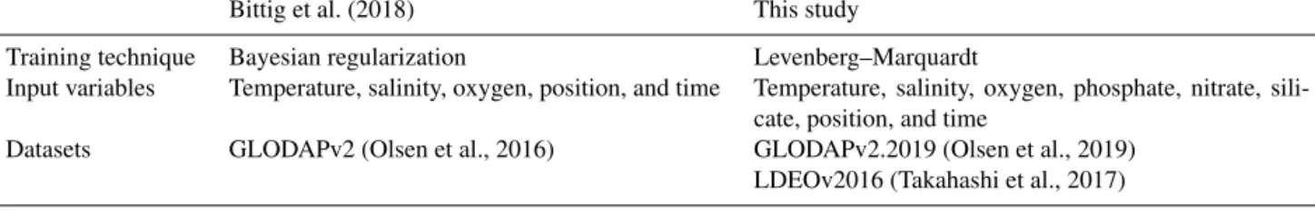
We compared our method with CANYON-B of Bittig et al. (2018), where TCO2values were also computed from multiple input variables. Both methods are based on neural networks but with certain differences as summarized in Ta- ble 1.

An error analysis was carried out in the same areas for which this was done by Broullón et al. (2019) for A_T and in several depth ranges (0–50, 50–200, 200–500, and 500–1000 m and 1000 m–bottom) for the two methods (our method and CANYON-B) and for the two datasets (Gv2QC and LDEO). The Gv2QC database was analyzed in this sec- tion instead of Gv2 because in the designing of CANYON-B only quality-controlled data were included. The analysis of CANYON-B using the LDEO dataset is useful to evaluate the validity of the approach followed by convertingpCO2

to TCO2 since CANYON-B has not been trained with this dataset.

ComputedpCO2fromATand TCO2derived from neural networks was also evaluated in the LDEO dataset to assess the adequacy of including this dataset in our approach and to assess the ability of NNGv2 of Broullón et al. (2019) and the present TCO₂neural network to compute other variables of the seawater CO₂system. Furthermore, we compared the magnitude of the errors with the ones obtained by Land- schützer et al. (2014), in whichpCO₂is computed directly with a neural network, to evaluate the accuracy of our com- putedpCO₂.

2.4 Validation

In addition to the ability to compute TCO₂ using the Gv2 and LDEO test sets, the neural network has been tested using independent data from 10 ocean time series, located in different regions of the world ocean (data were obtained from https://www.nodc.noaa.gov/ocads/oceans/time_series_

moorings.html, last access: 4 June 2019): Hawaii Ocean

(5)

Table 1.Differences between the methods used in the present study and in CANYON-B (Bittig et al., 2018).

Bittig et al. (2018) This study

Training technique Bayesian regularization Levenberg–Marquardt

Input variables Temperature, salinity, oxygen, position, and time Temperature, salinity, oxygen, phosphate, nitrate, silicate, position, and time

Datasets GLODAPv2 (Olsen et al., 2016) GLODAPv2.2019 (Olsen et al., 2019) LDEOv2016 (Takahashi et al., 2017)

Time-series (HOT ALOHA and HOT ALOHA SURFACE;

Dore et al., 2009), Bermuda Atlantic Time-series Study (BATS; Bates et al., 2012), European Station for Time-series in the Ocean at the Canary Islands (ESTOC; González- Dávila et al., 2010), Iceland Sea time series (ICELAND;

Olafsson et al., 2010), Irminger Sea time series (IRMINGER;

Olafsson et al., 2010), Kyodo North Pacific Ocean time series (KNOT; Wakita et al., 2010), K2 (Wakita et al., 2010), Ocean Weather Station Mike (OWS; Gislefoss et al., 1998), and Kerguelen Islands in the Indian sector of the Southern Ocean (KERFIX; Jeandel et al., 1998). CANYON-B was also used to compute TCO₂ in the time series to show the differences between that method and ours. The TCO₂ values were obtained by feeding the neural networks with the measured values of the input variables at each time series.

The data from these time series allow us to test the ability of the neural network to reconstruct not only the seasonal variability of TCO2at the various locations and depths sam- pled but also its long-term trends. For the trend analyses, the measured and estimated TCO2 values were deseasonalized following Bates et al. (2014).

As an additional test, the measuredpCO₂or thepCO₂calculated from measured TCO₂andA_Tat the time series stations was compared withpCO₂calculated from the neural- network-generated values of A_T and TCO₂. This provides insight into the combined performance of the NNGv2 of Broullón et al. (2019) and the neural network designed in the present study. Furthermore, we compared the magnitude of the errors to that obtained by Landschützer et al. (2014) for some of the time series.

2.5 Climatology ofTCO₂

We used the selected network, based on the results of the analyses described above, to construct a climatology of TCO2. Climatologies of the input variables were passed through the network to obtain the climatological fields of TCO₂. The spatiotemporal resolution of the product is determined by that of the climatologies used as inputs: 1^◦×1^◦horizontal resolution, 102 upper depth levels of the WOA13, and monthly (for 0–1500 m depth) to annual (for 1550–5500 m depth) temporal resolution. Temperature and salinity climatologies were obtained from objectively analyzed WOA13 fields (Locarnini et al., 2013; Zweng et al., 2013; https:

//www.nodc.noaa.gov/OC5/woa13/woa13data.html, last ac-

cess: 6 February 2017). Oxygen, phosphate, nitrate, and silicate climatologies were taken from Broullón et al. (2019; https://doi.org/10.20350/digitalCSIC/8644, last access: 1 August 2019). These climatologies of nutrients were created using the objectively analyzed climatologies of temperature, salinity, and oxygen (Garcia et al., 2014; oxygen climatology from WOA13 has been filtered by applying a fifth-order one-dimensional median filter through the depth dimension; see Broullón et al., 2019) from the WOA13 in CANYON-B (Bittig et al., 2018). As a year input is needed, we decided to center the TCO₂ climatology around 1995 based on the time distribution of the data used to create the WOA13 climatologies: the World Ocean Database 2013 (Boyer et al., 2013).

The computed climatological values were compared with those from measured data to assess the uncertainty of the climatology since the WOA13 does not offer an uncertainty field with the objectively analyzed climatologies. Un- fortunately, only two locations have enough measured data to calculate a pure climatological value of TCO2 for each month: HOT ALOHA and BATS. The measured values were monthly averaged at several depth levels, and the anthropogenic carbon as calculated by Lauvset et al. (2016) was added or subtracted to correct the data to the reference year of the climatology according to

TCO^year₂ ²=TCO^year₂ ¹−C_ant₂₀₀₂

(1+0.0191)^(year¹⁻²⁰⁰²⁾

−(1+0.0191)^year²⁻²⁰⁰²

, (2)

where TCO^year₂ ² is the TCO₂ corrected for year₂, which is the reference year of the climatology; TCO^year₂ ¹ is the TCO₂ measured in year₁, Cant₂₀₀₂ is the anthropogenic carbon for 2002; and 0.0191 is the annual increase rate derived from the scaling factor determined by Gruber et al. (2019) for the global ocean between 1994 and 2007.

We compared our climatology with previously published climatologies of TCO₂. The monthly surface climatology created by Takahashi et al. (2014) was used to assess the spatiotemporal differences in the surface layer. The annual climatology of Lauvset et al. (2016) was used to evaluate the spatial differences in the deeper parts of the ocean. For the comparisons, the climatologies of Takahashi et al. (2014) and Lauvset et al. (2016) were adjusted to the year 1995, subtract- ing the anthropogenic carbon (C_ant) of Lauvset et al. (2016) as in Eq. (2).

(6)

Finally, a surface climatology of pCO2 was computed from the TCO₂climatology of the present study and theAT

climatology of Broullón et al. (2019) to assess the potential of computing climatologies of other variables of the seawater CO₂system. For comparison, the updated monthlypCO₂ climatology from Landschützer et al. (2016, 2017) was used.

The values between 1981 and 2010 were averaged to obtain the climatological year 1995. The variable selected from Landschützer et al. (2017) was that labeled as spco2_raw (sea surfacepCO₂) in the netCDF file.

It should be noted that the RMSE and the bias were obtained for all the comparisons, the last statistic being computed as the difference between the measured (or computed by the method to compare) TCO2and the one obtained with the neural network of the present study.

3 Results

3.1 Neural network analysis

Following the established criteria to obtain the optimal number of neurons, the configuration with 128 neurons in the hidden layer was selected. From the 10 networks trained with this number of neurons for each approach (NNGv2LDEO and NNGv2QCLDEO), the ones with the lowest influence of the position input variables were selected. These two networks present a similar RMSE in both training and test datasets, showing there is no overfitting. Because in Gv2QC, both NNGv2LDEO and NNGv2QCLDEO produce the same global RMSE (6.1 µmol kg⁻¹), it is likely that the Gv2 dataset contains high-quality measurements, and the possible errors in the non-QC data of this dataset are clearly avoided by the network; otherwise NNGv2LDEO should have a higher RMSE in the test dataset than NNGv2QCLDEO because of an overfitting of the errors in the Gv2 dataset. The same holds for the LDEO dataset. The network properly fitted TCO₂ derived from the LDEO dataset since it does not significa- tively increase the global RMSE relative to a network only trained with Gv2. Therefore, we decided to continue with NNGv2LDEO only since it has fitted more relationships between variables (e.g., Gv2 has more data points than Gv2QC in the Mediterranean Sea), providing a more robust fitting.

For this network, the influence of each input variable on the computed TCO2 is depicted in Fig. S2. The position variables together (latitude, clongitude, slongitude, and depth) have no more than 30 % influence, allowing biogeochemical variables to be the main ones responsible for the variability of TCO₂. Furthermore, the input variable year has an influence lower than 5 %. This is probably responsible for capturing the positive interannual trend due to the TCO₂increase derived from anthropogenic emissions of CO₂to the atmosphere (see Sect. 3.2).

The global RMSE is quite low for the Gv2 dataset and for the LDEO dataset (Fig. 2). The measured and the computed data are highly correlated (Fig. 2), and the bias is negligi-

ble in both datasets. The higher RMSE in the LDEO dataset likely results from the higher variability of TCO₂ in the surface layer and from uncertainties in its calculation from pCO₂.

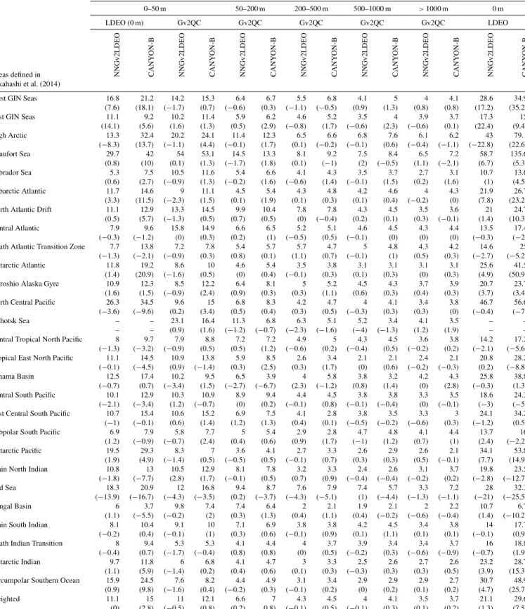
The RMSE by area and depth for NNGv2LDEO and CANYON-B in Gv2QC is shown in Table 2. The highest errors for the two methods are in the 0–50 m layer for the Gv2QC dataset and the LDEO dataset. These errors get smaller with increasing depth for all areas, and the depth- weighted RMSE of the two methods is not significantly different below 50 m. In the LDEO dataset, NNGv2LDEO pro- duces a lower error than CANYON-B, except for two areas: East GIN (Greenland, Iceland, and Norwegian) Seas and the Bengal Basin (Table 2), although there are only 9 and 13 data points, respectively, in each area. Interest- ingly, CANYON-B is able to reproduce the TCO2data derived from the complete LDEO dataset with a lower error than the one it obtains for the complete Gv2QC dataset in the surface ocean (RMSE LDEO: 16.4 µmol kg⁻¹; RMSE Gv2QC, 0–5 m: 17.8 µmol kg⁻¹), supporting the approach of computing reliable TCO₂ values from thepCO₂ of the LDEO dataset and theA_T computed with NNGv2 (Broul- lón et al., 2019) since CANYON-B was not trained with the LDEO database. A similar result was obtained for NNGv2LDEO but with a higher difference between the two errors (RMSE LDEO: 11.4 µmol kg⁻¹; RMSE Gv2QC, 0–

5 m: 17.1 µmol kg⁻¹). Finally, the surface RMSE towards LDEO data of NNGv2LDEO is clearly lower than that of CANYON-B. This shows the value of including pCO2- derived surface TCO2 among the training data, through which there are more fitted relations in our new method.

For data from Gv2 where no QC was performed for at least one of the variables used in the present study (Gv2noQC), the RMSE also decreases with increasing depth ( <50 m: 22.5 µmol kg⁻¹; 50–200 m: 9.8 µmol kg⁻¹; 200–

500 m: 7 µmol kg⁻¹; 500–1000 m: 5.4 µmol kg⁻¹;>1000 m:

5.4 µmol kg⁻¹). Thus, the error in Gv2noQC is similar to that in the areas with the highest error in Gv2QC (Table 2; except in Beaufort Sea, where the error is considerably higher).

However, the higher error in Gv2noQC is mainly caused by the samples located in the Arctic Ocean since cruises in the Atlantic and Pacific oceans are modeled with a very low error. Therefore, using Gv2noQC does not imply the introduction of low-quality data in our study; otherwise the network would not compute TCO2 with low errors in Gv2QC because of an overfitting of the possible low-quality data that Gv2noQC could contain.

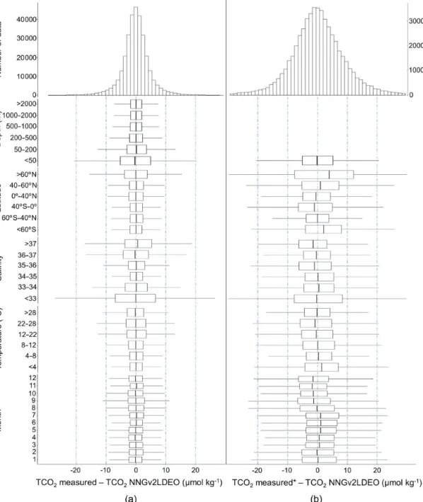
In general, the highest differences between measured and estimated TCO₂ occurs in the high-latitude surface oceans (Figs. 3 and 4). In Gv2, 40 % of the samples with differences beyond±3RMSE (3 times RMSE; threshold selected to refer to samples with large residuals) are at latitudes greater than 70^◦N. In the LDEO dataset, 39 % of the samples with differences beyond±3RMSE are from latitudes south of 70^◦S.

These samples where RMSE is high are 7.5 % of the total

(7)

Figure 2.Regression of TCO₂computed using NNGv2LDEO and TCO₂in Gv2 and the LDEO dataset. The graph is divided into pixels.

The color of each pixel is determined by the number of points inside it. Note the logarithmic scale of the pixels accounting for the large number of data.

Figure 3.Differences between(a)Gv2 TCO₂and NNGv2LDEO TCO₂(0–30 m) and(b)LDEO TCO₂and NNGv2LDEO TCO₂(0 m).

This figure was made with Ocean Data View (Schlitzer, 2016).

north of 70^◦N in Gv2 and 42 % of the total south of 70^◦S in the LDEO dataset. The samples with low salinities have the highest errors (Fig. 4). A total of 41.5 % of the samples in Gv2 and 43 % in the LDEO dataset with differences beyond±3RMSE have salinities below 33. Furthermore, in the LDEO dataset, the number of samples with residuals beyond

±3RMSE increases with increasing SD of bothpCO2and salinity in the monthly averaging in each pixel in the LDEO subset (Fig. S3). This result shows the difficulty of modeling areas with a high submonthly variability inpCO₂and salinity and supports the exclusion of the averaged LDEO data with a high SD since it could cause the network to interpret the submonthly variability as monthly variability (note that the purpose of this study is to capture the monthly variability).

Like for modeling A_T (Takahashi et al., 2014; Broullón et al., 2019), the Arctic Ocean is one of the regions with the highest RMSE of neural-network-estimated TCO2. The

major Arctic rivers contribute TCO₂concentrations ranging between 400 and 3600 µmol kg⁻¹(estimated by Tank et al., 2012), derived mainly from carbonated rocks in the water- sheds. Other areas like the Okhotsk Sea also show a high RMSE (Table 2 and Fig. 3), probably because of the high riverine input of TCO2 (Watanabe et al., 2009). An input variable accounting for the contribution of the rivers to the TCO₂pool would improve the neural network performance in areas like these, but it is not available.

The errors of thepCO₂ computed in the LDEO dataset with TCO₂ from NNGv2LDEO and A_T from NNGv2 (Broullón et al., 2019) are similar to the errors obtained by Landschützer et al. (2014) for the SOCAT database in some of the areas (10–16 µatm; Table 2). This result shows the potential of computingpCO₂ values with neural networks trained for other variables of the seawater CO₂ system, at least in some ocean regions. The global error of thepCO₂ in the LDEO dataset is clearly higher than that obtained by

(8)

Table 2.RMSE (bias) by area and depth for TCO₂and pCO₂, computed with CANYON-B and NNGv2LDEO in Gv2QC and LDEO datasets. For each depth range, the RMSE (bias) in each area was weighted by the contribution of its data to the total. Units are micromoles per kilogram (µmol kg⁻¹) for TCO₂and microatmospheres (µatm) forpCO₂.

TCO₂ pCO₂

0–50 m 50–200 m 200–500 m 500–1000 m >1000 m 0 m

LDEO (0 m) Gv2QC Gv2QC Gv2QC Gv2QC Gv2QC LDEO

Areas defined in NNGv2LDEO CANYON-B NNGv2LDEO CANYON-B NNGv2LDEO CANYON-B NNGv2LDEO CANYON-B NNGv2LDEO CANYON-B NNGv2LDEO CANYON-B NNGv2LDEO CANYON-B Takahashi et al. (2014)

West GIN Seas 16.8 21.2 14.2 15.3 6.4 6.7 5.5 6.8 4.1 5 4 4.1 28.6 34.9

(7.6) (18.1) (−1.7) (0.7) (−0.6) (0.3) (−1.1) (−0.5) (0.9) (1.3) (0.8) (0.8) (17.2) (35.2)

East GIN Seas 11.1 9.2 10.2 11.4 5.9 6.2 4.6 5.2 3.5 4 3.9 3.7 17.3 15

(14.1) (5.6) (1.6) (1.3) (0.5) (2.9) (−0.8) (1.7) (−0.6) (2.3) (−0.6) (0.1) (22.4) (9.4)

High Arctic 13.3 32.4 20.2 24.1 11.4 12.3 6.5 6.6 6.8 7.6 6.1 6.2 43 79.1

(−8.3) (13.7) (−1.1) (4.4) (−0.1) (1.7) (0.1) (−0.2) (−0.1) (0.6) (−0.4) (−1.1) (−22.8) (22.6)

Beaufort Sea 29.7 42 54 53.1 14.5 13.3 8.1 9.2 7.5 8.4 6.5 7.2 58.7 135.6

(0.8) (10) (0.1) (1.3) (−1.7) (1.8) (0.1) (−1) (2) (−0.5) (1.1) (−2.1) (6.7) (5.3)

Labrador Sea 5.3 7.5 10.5 11.6 5.4 6.6 4.1 4.3 3.5 3.7 2.7 3.1 10.7 13.6

(0.6) (2.7) (−0.9) (1.3) (−0.2) (1.6) (−0.6) (1.4) (−0.1) (1.5) (0.2) (1.6) (1) (4.5)

Subarctic Atlantic 11.7 14.6 9 11.1 4.5 5.4 4.3 4.8 4.2 4.6 4 4.3 21.9 26.7

(3.3) (11.5) (−2.3) (1.5) (0.1) (1.9) (0.1) (0.3) (0.1) (0.4) (−0.2) (0) (7.8) (23.2)

North Atlantic Drift 11.1 12.9 13.3 14.5 9.9 10.4 7.8 7.8 4.3 4.5 3.5 3.6 21 24.7

(0.5) (5.7) (−1.3) (0.5) (0.7) (0.5) (0) (−0.4) (0.2) (0.1) (0.3) (−0.1) (1.4) (10.3)

Central Atlantic 7.9 9.6 15.8 14.9 6.6 6.5 5.2 5.1 4.6 4.5 4.3 4.4 13.5 17.4

(−0.3) (−1.2) (0) (0.3) (0.2) (1) (−0.5) (0.5) (−0.1) (0) (0) (0) (−0.3) (−2)

South Atlantic Transition Zone 7.7 13.8 7.2 7.8 5.4 5.7 5.7 4.7 5 4.8 4.3 4.2 14.6 25

(−1.3) (−2.1) (−0.9) (0.3) (0.8) (0.1) (1.1) (0.7) (−0.1) (1) (0.5) (0.3) (−2.7) (−5.2)

Antarctic Atlantic 11.8 19.2 8.6 10 4.6 5.4 3.5 3.8 3.1 3.1 3.1 3.1 25.6 41.5

(1.4) (20.9) (−1.6) (0.5) (0) (0.4) (−0.1) (0.3) (0.1) (0.3) (0) (0.3) (4.9) (50.9)

Kuroshio Alaska Gyre 10.9 12.3 8.5 12.2 6.4 8.1 5 5.2 4.5 4.3 3.7 3.9 20.7 23.7

(1.6) (1.5) (−0.9) (2.4) (0.9) (0.3) (0.3) (1.1) (0.6) (0.3) (0.4) (0.3) (3.7) (3.4)

North Central Pacific 26.3 34.5 9.6 15 6.8 8.3 4.2 4.7 4 4.1 3.4 3.8 46.7 56.6

(−3.6) (−9.6) (0.2) (3.4) (0.5) (0.4) (0.3) (0.5) (−0.3) (0.3) (0.3) (0) (−0.4) (−7)

Okhotsk Sea – – 23.1 16.4 11.3 6.8 6.3 5.1 5.2 3.4 4.1 3.5 – –

– – (0.9) (1.6) (−1.2) (−0.7) (−2.3) (−1.6) (−4) (−1.3) (1.2) (1.9) – –

Central Tropical North Pacific 8 9.7 7.9 8.8 7.2 7.2 4.9 5 4.3 4.5 3.6 3.8 14.2 17.2

(−1.3) (−3.2) (−0.9) (0.5) (0.5) (1.2) (−0.6) (0.2) (−0.4) (0.5) (−0.2) (0.2) (−2.1) (−5.6)

Tropical East North Pacific 11.1 14.5 10.9 13.8 5.9 8.5 2.6 3.4 2.1 2.1 2.4 2.1 20.8 28.2

(−0.1) (−4.5) (0.9) (−1.4) (0.3) (2.5) (0.3) (1.7) (0) (0.6) (−0.2) (−0.3) (0.2) (−8.8)

Panama Basin 12.5 17.4 10.2 9.5 6.5 3.9 4 5.8 3.8 3.2 4.2 4.3 25.8 38.8

(−0.7) (0.7) (−3.4) (1.5) (−2.7) (−6.7) (2.3) (−1.2) (0.8) (1.4) (0) (2.8) (−0.3) (1.3)

Central South Pacific 10.1 12.9 10.3 10.9 8.9 9.4 4.4 4.5 3.8 3.8 3.3 3.5 18.6 24.3

(−2.1) (−3.4) (1.2) (−0.7) (0) (0.2) (−0.1) (0.8) (−0.1) (−0.4) (0) (−0.1) (−3) (−5)

East Central South Pacific 10.7 15.4 10.6 15.2 6.9 7.5 4.1 2.8 3.8 3.5 3.3 3 24.1 34.2

(−1) (−0.1) (0.6) (1.4) (1.2) (1.3) (0.4) (0.1) (−0.5) (−0.2) (−0.6) (0.3) (−1.2) (0.5)

Subpolar South Pacific 6.9 7.9 5.8 7.7 5 5.4 2.9 2.8 4.7 4.8 4.1 4.4 13.7 16

(1.2) (−0.9) (−0.7) (2.4) (0.4) (0.6) (0.9) (1.7) (−1) (1.2) (0.7) (1) (2.4) (−2.2)

Antarctic Pacific 19.5 29.3 8.3 7 3.6 4.1 2.7 3.3 2.6 2.9 2.6 2.1 34.1 53.8

(1.9) (4.9) (−1.4) (0.5) (−0.5) (0.5) (−0.1) (0.7) (0.3) (0.3) (0.5) (−0.1) (7.7) (14.9)

Main North Indian 10.8 13 10.5 12.9 8.1 7.8 3.2 3.3 2.4 2.6 3.1 3.7 19.8 23.5

(−1.8) (−7.7) (2.8) (1.7) (−0.1) (0.5) (0.7) (0.9) (−0.4) (−0.4) (−0.2) (0.2) (−2.8) (−12.7)

Red Sea 18.3 20.9 12 16.8 9.4 8.7 7.6 7.9 7.4 5.7 3.3 7.2 28 32.3

(−13.9) (−16.7) (−4.3) (−3.5) (0.2) (−3.7) (−4.3) (−5.1) (1) (−4.4) (−1.3) (−1.1) (−21) (−25.5)

Bengal Basin 6 3.7 9.8 7.4 7.4 6.4 2 2.1 1.9 2.1 2 2.2 10.7 6.7

(1.1) (−5.5) (−0.2) (2) (0.3) (1.3) (0.4) (1.1) (0.4) (−0.2) (−0.6) (−0.4) (1.4) (−10.2)

Main South Indian 8.1 10.4 9.1 10 7.1 6.9 3.8 3.8 4.2 4.5 3.4 3.8 14 17.7

(−0.2) (0.4) (−0.1) (1) (0.3) (0.6) (−0.1) (0.9) (0.1) (1.1) (0.1) (0.1) (−0.1) (0.9)

South Indian Transition 8 9.4 5.3 5.3 4.1 4.4 4 3.7 3.9 3.4 3.4 3.7 16 18.8

(−0.4) (0.7) (−1.7) (−0.4) (0.8) (0.8) (0) (0.5) (−0.2) (0.3) (−0.6) (−0.9) (−0.7) (1.9)

Antarctic Indian 9.7 11.8 6 6.8 4.1 4.7 3 3.3 2.5 2.6 2.7 2.6 23.2 28.7

(1.1) (5.9) (−1.4) (0.2) (0.4) (0.6) (0.1) (0.3) (−0.3) (0.3) (0.3) (0.5) (3.9) (15.3)

Circumpolar Southern Ocean 15.9 24.5 7.6 8.2 4.4 4.9 3.1 3.4 2.9 2.9 2.9 2.7 30.7 48.9

(0.9) (9.8) (−1.6) (0.4) (−0.2) (0.3) (−0.1) (0.2) (0) (0.2) (0.1) (0.2) (4.7) (25.7)

Weighted 11.1 15 11 12.1 6.6 7 4.3 4.5 4 4.1 3.5 3.7 21.1 29.6

(0) (2.8) (−0.5) (0.8) (0.2) 0.8) (−0.1) (0.5) (−0.1) (0.3) (0.1) (0.2) (1.3) (7.5)

(9)

Figure 4. Histograms and box plots of differences between measured and neural-network-computed TCO₂in (a)Gv2 and(b) LDEO.

∗TCO₂computed from measuredpCO₂and neural-network-derivedA_T.

Landschützer et al. (2014) for the SOCAT dataset (22 vs.

12 µatm, respectively), although the critical areas are mainly the same (Fig. S4): equatorial Pacific upwelling system, Arc- tic and subarctic waters around the Alaska Peninsula, the Southern Ocean, the Gulf Stream, and the North Atlantic Current. At this point, the following should be considered:

(1) thepCO₂computed in the present study is derived from A_Tand TCO₂and not from specific modeling forpCO₂, and therefore it contains errors associated with this computation (∼6 µatm; Millero, 1995) and the neural network estimates of A_T and TCO₂; (2) the present study includes the Arc-

tic region where the highest errors occur (Table 2; Beaufort Sea and High Arctic areas); and (3) there is a longer temporal range in the present study (1973–2016). The analysis of Landschützer et al. (2014) in the LDEO dataset for data that differ from SOCAT shows a global error higher than the one obtained in the present study for all LDEO data between 1998 and 2011 (25.9 vs. 21.3 µatm, respectively). The error between 40^◦S and 40^◦N is similar in the two studies (Land- schützer et al., 2014: 16.5 µatm; NNGv2LDEO: 16.4 µatm).

Although it is not the main objective of this work, these last two results show how NNGv2LDEO and NNGv2 (Broullón

(10)

et al., 2019) have the potential to computepCO2values between 40^◦S and 40^◦N with similar errors as the method with the lower error in thepCO₂modeling to obtain a climatology and with lower errors in high latitudes for the LDEO dataset, even taking into account the inclusion of the critical area of the Arctic in the computation of the error of thepCO₂from the present study (it is not included in Landschützer et al., 2014) and the higher number of data from high latitudes in the present study (15 479 vs. 3799).

3.2 Time series validation

The good generalization of the network in the test dataset containing data from Gv2 and the LDEO dataset with a similar RMSE as the one reached in the training set is also evidenced through independent time series data (Table 3).

Except for KERFIX, where the number of data points is very low and Olsen et al. (2019) suggested an adjustment to the original data of−39 µmol kg⁻¹, TCO₂computed using NNGv2LDEO and CANYON-B at the time series locations is characterized by low errors and biases (Table 3).

NNGv2LDEO computes TCO₂with a lower RMSE and bias than CANYON-B for most of the time series stations (Ta- ble 3). CANYON-B reaches a lower RMSE in HOT ALOHA SURFACE and ESTOC than NNGv2LDEO, but the bias is considerably higher in these time series for CANYON-B.

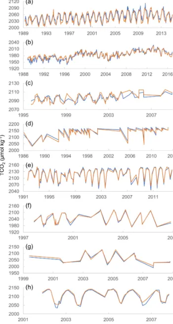
The seasonal variability is well captured by NNGv2LDEO, showing its great potential to design a monthly climatology. In the surface layer, where the seasonal variability is the highest, the computed values are strongly correlated with the measured TCO2in all the time series (Fig. 5). In addition, the high correlation holds for all depths (Table S1). The TCO₂computation with a low error in these time series located in different oceanic regimes as well as in the areas of Table 2 shows the good performance of NNGv2LDEO in almost any region of the ocean.

Assessing the potential of neural networks to obtain values of other variables of the seawater CO₂system in the time series,pCO₂calculated withA_Tfrom NNGv2 (Broullón et al., 2019) and TCO₂from NNGv2LDEO compared quite well withpCO₂as measured or calculated fromA_Tand TCO₂at the time series stations (Table 4). Except for BATS, thepCO2

obtained in the present study has a lower error than that re- ported by Landschützer et al. (2014; Table 4). In contrast, the bias in the present study is higher, except for ESTOC. Con- sidering the error involved in the calculation ofpCO2from AT and TCO₂ (∼6 µatm); Millero, 1995), and the error in the computed AT and TCO₂ with the neural networks (Ta- ble 4), our results demonstrate again the ability of NNGv2 and NNGv2LDEO to calculate other variables of the seawater CO₂system with a relatively low error.

Using NNGv2LDEO, it is also possible to reproduce the secular trends in TCO₂. Using seasonal detrending to en- hance the multiannual changes, similar trends in the longer time series are found for the measured TCO₂and the neural-

Figure 5.Measured (blue line) and computed (orange line) TCO₂ with NNGv2LDEO for the depth range 0–15 m (0–30 m in panel b) for several time series.(a)BATS,(b)HOT ALOHA SURFACE, (c)ESTOC,(d)ICELAND,(e)IRMINGER,(f)KNOT,(g)K2 and (h)OWS.

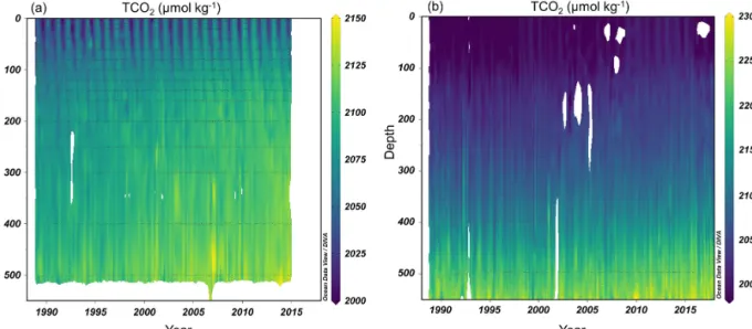
network-computed TCO2 (Table 5). The same holds for pCO₂ (Table 5), although at the IRMINGER site the trend obtained from the neural-network-generated data is significantly lower than that from measured data. The neural networks seem to capture the anthropogenic influence in the seawater CO₂system and thus the ocean acidification process (Fig. 6). Furthermore, using NNGv2LDEO increases the number of TCO₂ data where the various inputs were measured but not TCO₂itself. This allows for the evaluation of high-frequency changes (Fig. 6) and for the calculation of

(11)

Table 3.RMSE and bias between measured and computed TCO₂concentrations in several time series. The comparison was done using only water samples where all the input variables for NNGv2LDEO and the TCO₂were measured in the same water sample.

NNGv2LDEO CANYON-B

Time series Location Time period n RMSE Bias RMSE Bias

(µmol kg⁻¹) (µmol kg⁻¹) (µmol kg⁻¹) (µmol kg⁻¹)

BATS 31.7^◦N, 64.2^◦W 1988–2014 4121 7.7 0.1 7.7 −0.6

HOT ALOHA 22.8^◦N, 158^◦W 1988–2017 4054 5.4 −0.5 5.1 −2

HOT ALOHA SURF 22.8^◦N, 158^◦W 1988–2016 281 6.3 −1.6 5.8 −5.1

ESTOC 29.3^◦N, 15.5^◦W 1995–2008 1697 7.1 0.8 6.6 4.7

ICELAND 68^◦N, 12.7^◦W 1985–2013 1322 5.4 5.6 6.9 5.3

IRMINGER 64.3^◦N, 28^◦W 1991–2013 1086 4.8 3.3 7.5 6.6

K2 47^◦N, 160^◦E 1999–2008 615 3.6 1.3 6.3 2.4

KNOT 44^◦N, 155^◦E 1997–2008 1321 5.8 −0.8 7.2 −1.9

OWS 66^◦N, 2^◦E 2001–2007 803 6.8 −1 10.5 −4.7

KERFIX 50.4^◦S, 68.2^◦E 1992–1994 38 13.2 26.4 13.1 28.9

Table 4.RMSE and bias between measuredpCO₂(and in some cases, computed from measuredA_Tand TCO₂in time series wherepCO₂ was not measured) and computedpCO₂withA_Tfrom NNGv2 (Broullón et al., 2019) and TCO₂from NNGv2LDEO in several time series.

The time period forpCO₂from this study is the same as in Table 3. Consult Table 2 in Landschützer et al. (2014) for its time period. The depth range is 0–15 m. Only time series with more than 30 data points are included. RMSE and bias for computedA_Twith NNGv2 (Broullón et al., 2019) and TCO₂with NNGv2LDEO are included to show the errors in the variables used to compute TCO₂.

pCO₂ A_T TCO₂

NNGv2LDEO Landschützer et al. (2014) NNGv2 (Broullón et al., 2019) NNGv2LDEO

Time series RMSE Bias RMSE Bias RMSE Bias RMSE Bias

(µatm) (µatm) (µatm) (µatm) (µatm) (µatm) (µatm) (µatm)

BATS 17.2 9.7 15.6 0.4 5.6 −1.7 10.1 4.4

HOT ALOHA SURF 10.3 −3.6 11.6 0.1 5.0 0.9 6.5 −1.6

ESTOC 10.6 2.7 14.5 −7.1 2.6 −2.7 5.3 −0.6

ICELAND 16 14.8 – – 5.4 0.7 5.4 5.4

IRMINGER 13.1 −1.8 22.6 −1.1 7.0 −0.4 6.6 −1.1

K2 18.1 −3.2 27.8 −0.2 5.1 −0.5 5.7 −2.4

KNOT 20.8 8.6 – – 6.6 −7.3 8.2 −2.5

interannual trends with a low error (as temporal sampling biases are reduced).

3.3 Climatology

Using NNGv2LDEO we have demonstrated its ability to compute TCO2values with low errors and especially to capture the monthly variability of this variable. In addition, the climatologies of the input variables used to create the climatology of TCO₂have been satisfactorily evaluated previously for the construction of anAT climatology (Broullón et al., 2019). Considering these results, a monthly climatology of TCO₂is obtained by passing the input climatologies through NNGv2LDEO.

The spatial distribution of the surface annual mean climatology of TCO₂ (Fig. 7a) is similar to two recent climatologies: those of Takahashi et al. (2014) and Lau- vset et al. (2016). The largest surface TCO₂ concentra-

tions occur in the Southern Ocean, subpolar North Atlantic, Nordic Seas, and Mediterranean Sea (note that the latter is not included in these other climatologies). In general, surface TCO₂ decreases from high to low latitudes. The Indian and the Pacific oceans are characterized by lower concentrations of TCO₂ at higher latitudes than the At- lantic, the latter being the ocean with the highest surface TCO2 by area. TCO2 increases with depth in all oceans, in particular in the upwelling regions, where this increase is expanded eastwards with depth (Fig. 7b and video at https://doi.org/10.20350/digitalCSIC/10551, Broullón et al., 2020). Depending on the area, the values reach a maximum at certain intermediate depths, and below it the concentration gradually decreases or remains almost constant (Fig. S5).

The largest seasonal variability occurs at the surface at high latitudes, in the Pacific upwelling region, the equatorial African coasts, and in the area under influence of the Amazon River (Fig. 8a). At depth, the seasonal variability de-

(12)

Table 5.Long-term trends (seasonally detrended) of the measured and computed TCO₂andpCO₂from neural networks at time series locations in the depth range 0–15 m.

TCO₂(µmol kg⁻¹yr⁻¹) pCO₂(µatm yr⁻¹) Time series Measured Computed Measured^∗ Computed

BATS 1.2 1.1 1.8 1.7

HOT ALOHA SURF 1.7 1.3 1.8 1.4

ICELAND 0.9 0.9 1.5 1.6

IRMINGER 0.6 0.5 2.5 1.7

∗Computed from measuredA_Tand TCO₂in time series wherepCO₂was not measured.

Figure 6. Time series of TCO₂using NNGv2LDEO at(a)BATS and(b)HOT ALOHA locations. The water column shows a higher concentration of TCO₂year by year. This figure was made with Ocean Data View (Schlitzer, 2016).

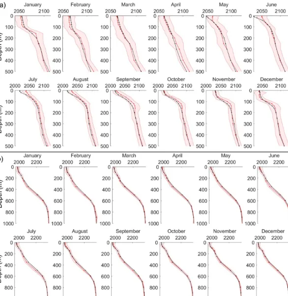
creases, except for the Pacific upwelling region, where it increases and moves progressively northward between 30 and 150 m (Fig. 8b). This increase is correlated with the high seasonal variability of the climatologies of nutrients, oxygen, and temperature at these depths. Czeschel et al. (2012) also showed an increase in the subsurface variability of oxygen from measured profiles. Similar increases also occur in the Indian Ocean north of 20^◦S between 50 and 100 m and in the equatorial Atlantic Ocean in the same depth range. At the 1500 m level, the seasonal variability is below 10 µmol kg⁻¹ in most of the ocean (Fig. 8c). This last result shows that an annual climatology below 1500 m is sufficient.

Although the surface patterns of the annual mean of the TCO2climatology are very similar to those of the other recent climatologies (Takahashi et al., 2014; Lauvset et al., 2016), differences do occur. The annual mean climatology of the present study is closest to that of Takahashi et al. (2014;

Table 6). The largest differences between these two climatologies are located in the Arctic, North Pacific, Peru upwelling area, western South Pacific, and the area of influence of the Antarctic Circumpolar Current (Fig. S6a). The

Atlantic and the Indian oceans do not show significant differences. Our climatology shows more deviations from that of Lauvset et al. (2016), compared in the grid of Takahashi et al. (2014; Table 6). The highest differences are found in the North Pacific, around Antarctica, the Nordic Seas, the South and North Atlantic, and in several less localized areas around the oceans (Fig. S6b). When the climatology of Takahashi et al. (2014) is compared to that of Lauvset et al. (2016), the differences are even higher (Table 6), and the critical areas are the same of those of the previous comparison. Although it is clear that discrepancies between the three climatologies are derived from the different methods used, the higher sim- ilarity between ours and the one of Takahashi et al. (2014) is probably due to the influence of the same source used to create them, the World Ocean Atlas.

The comparison of our climatology with that of Lauvset et al. (2016) at the 33 depth levels of Lauvset et al. (2016) shows a reduction in the RMSE with depth. Between 0 and 1000 m, the RMSE is reduced from∼32 to 7 µmol kg⁻¹(Ta- ble S2; note the higher RMSE at surface compared to the one obtained for the grid of Takahashi et al., 2014, because of

(13)

Figure 7.Annual mean climatology of TCO₂at(a)0 m,(b)100 m, and(c)1000 m. This figure was made with Ocean Data View (Schlitzer, 2016).

Figure 8.Seasonal amplitude of TCO₂at(a)0 m,(b)100 m, and(c)1500 m. The contour lines of 25, 50, 75, and 100 µmol kg⁻¹are shown.

This figure was made with Ocean Data View (Schlitzer, 2016).

the inclusion of areas which are not included in the latter’s grid, and the difficulty of modeling TCO₂in some areas, like the Arctic and the Mediterranean Sea). This reduction with depth is probably due to the reduction in the variability in most of the ocean below the surface. The surface values in Lauvset et al. (2016) are likely characteristic of months in which most of the sampling was carried out. Because of the lower variability of TCO2at depth, the values are closer to the annual mean, and therefore the two compared climatologies are more similar at depth than at surface depth levels.

Below 1000 m, the differences between the two climatologies

are not significant, with an RMSE around 5 µmol kg⁻¹and a bias around 0.5 µmol kg⁻¹at each depth level (Table S2).

Our monthly climatology shows a high correspondence with that of Takahashi et al. (2014), although the RMSE values show that there are also large differences in certain areas (Table 7). These areas are mainly the same as those in the comparison of the annual mean climatologies, but some other small regions with high differences appear for each month all through the ocean (Fig. S7).

Unfortunately, the uncertainty of the TCO2 climatology cannot be assessed globally and robustly. As Broullón et al. (2019) stated, the unavailability of an uncertainty field