The Circulation Response to Volcanic Eruptions: The Key Roles of Stratospheric Warming and Eddy Interactions
KEVINDALLASANTA ANDEDWINP. GERBER
Center for Atmosphere–Ocean Science, Courant Institute of Mathematical Sciences, New York University, New York, New York
MATTHEWTOOHEY
GEOMAR Helmholtz Centre for Ocean Research Kiel, Kiel, Germany
(Manuscript received 21 February 2018, in final form 27 November 2018) ABSTRACT
Proxy data and observations suggest that large tropical volcanic eruptions induce a poleward shift of the North Atlantic jet stream in boreal winter. However, there is far from universal agreement in models on this effect and its mechanism, and the possibilities of a corresponding jet shift in the Southern Hemisphere or the summer season have received little attention. Using a hierarchy of simplified atmospheric models, this study examines the impact of stratospheric aerosol on the extratropical circulation over the annual cycle. In par- ticular, the models allow the separation of the dominant shortwave (surface cooling) and longwave (strato- spheric warming) impacts of volcanic aerosol. It is found that stratospheric warming shifts the jet poleward in both the summer and winter hemispheres. The experiments cannot definitively rule out the role of surface cooling, but they provide no evidence that it shifts the jet poleward. Further study with simplified models demonstrates that the response to stratospheric warming is remarkably generic and does not depend critically on the boundary conditions (e.g., the planetary wave forcing) or the atmospheric physics (e.g., the treatment of radiative transfer and moist processes). It does, however, fundamentally involve both zonal-mean and eddy circulation feedbacks. The time scales, seasonality, and structure of the response provide further insight into the mechanism, as well as its connection to modes of intrinsic natural variability. These findings have implications for the interpretation of comprehensive model studies and for postvolcanic prediction.
1. Introduction
Volcanic aerosols primarily impact Earth’s climate by scattering incoming shortwave radiation and absorbing and emitting longwave radiation. While aerosol in the troposphere is generally washed out by the hydrological cycle within a few weeks, sufficiently large eruptions can inject material into the stratosphere. In particular, the most influential eruptions on global climate are large tropical eruptions (e.g.,Robock and Mao 1995;Robock 2000). Volcanoes emit both ash and sulfuric compounds that oxidize and form sulfuric acid aerosol droplets; it is thought that the latter is most important in the stratosphere (Robock 2000). Following large tropical eruptions, like that of Mt. Pinatubo in 1991, the Brewer–
Dobson circulation, or meridional overturning circula- tion of the stratosphere, lifts and meridionally spreads
these droplets (Trepte et al. 1993;Hitchman et al. 1994), allowing them to persist in the middle atmosphere with ane-folding lifetime of approximately one year (Barnes and Hofmann 1997). The shortwave effect causes glob- ally averaged surface cooling, while the longwave effect causes localized warming of the tropical stratosphere (Robock 2000). The cooling effect of volcanic eruptions has been appreciated for centuries (e.g.,Franklin 1784) but, paradoxically, temperature reconstructions from proxy data also indicate that much of northern Eurasia warms during the first winters after a large volcanic eruption, even after accounting for El Niño–Southern Oscillation (ENSO) variability (Robock and Mao 1995;
Fischer et al. 2007).
Reconstructions of Northern Hemisphere (NH) tem- perature changes following past eruptions show spatial patterns reminiscent of a positive anomaly of the northern annular mode (e.g.,Robock 2000;Christiansen 2008). A positive annular mode is characterized by a poleward shift
Corresponding author: Kevin DallaSanta, dalla@cims.nyu.edu DOI: 10.1175/JCLI-D-18-0099.1
Ó2019 American Meteorological Society. For information regarding reuse of this content and general copyright information, consult theAMS Copyright Policy(www.ametsoc.org/PUBSReuseLicenses).
have found a poleward shift of the SH winter jet (e.g., Karpechko et al. 2010; McGraw et al. 2016) while again others have found little or opposite response (e.g.,Robock et al. 2007;Roscoe and Haigh 2007).
In the context of a large tropical eruption, a poleward jet shift has been attributed to two general mechanisms:
surface dimming (the shortwave effect) and stratospheric warming (the longwave effect). A first possible mecha- nism (Graf 1992;Stenchikov et al. 2002) is that aerosol scattering of shortwave radiation dims and cools the surface, reducing the tropospheric meridional tempera- ture gradient. Assuming this reduces midlatitude baro- clinicity, it is possible that upward wave flux is reduced so as to stimulate a stronger stratospheric vortex, which in turn drives a poleward shift of the jet, as observed with natural variability (Baldwin and Dunkerton 2001).
A second possible mechanism (Robock and Mao 1995) observes that aerosol absorption of longwave radiation warms the tropical stratosphere, steepening the strato- spheric meridional temperature gradient. At a small Rossby number, this balances a westerly acceleration of the zonal winds. Assuming this acceleration occurs in the midlatitudes, the vortex acceleration feeds back with a poleward shift of the jet via the stratosphere–
troposphere coupling reflected in the annular mode. A majority of previous studies have favored this hypoth- esis; however, as has been noted (Stenchikov et al. 2002;
Toohey et al. 2014;Bittner et al. 2016b), the meridional temperature gradient may not be in direct balance with a strengthened vortex. We will constructively demon- strate that the qualitative nature of this hypothesis is quite sensitive to its quantitative details.
Given the wide variety of results obtained with com- prehensive models and the inconsistent conclusions re- garding mechanisms,Zanchettin et al. (2016)proposed a volcanic model intercomparison project (VolMIP) to study this issue within phase 6 of the Coupled Model Intercomparison Project (CMIP6). VolMIP details sev- eral experiments, including differentiation of forcings (stratospheric warming and surface dimming). The unified protocol will reduce methodological uncertainty in our understanding of the response and afford the opportunity
previous model studies with one another.
We seek to address this challenge by examining vol- canic forcing comparable to a large tropical eruption in a hierarchy of idealized models, sequentially studying how each level of complexity relates to the response.
The resultant simplicity aids understanding of the dy- namical mechanism of volcanic forcing although, as we will see, causality is not always clear in the nonlinear atmosphere.
We first investigate the equilibrium responses to the two aerosol impacts in an idealized moist atmospheric model, which includes a representation of zonal asym- metries in the surface conditions. We find that the model’s circulation response is driven by tropical stratospheric warming, not surface cooling associated with a reduction of insolation. Next, we simplify our model in order to understand the mechanistic roles played by planetary-scale waves, radiative transfer and moist physics, synoptic eddy feedbacks, and the zonal- mean circulation. Additional insight into the mechanism is provided by the temporal evolution in response to instantaneous forcing. Finally, we will relate the forced response of these models to their internal modes of variability.
2. An idealized atmospheric model
We start with the equilibrium response to solar dim- ming and stratospheric warming in a recently developed moist atmospheric model, Model of an Idealized Moist Atmosphere (MiMA), which is described in detail by Jucker and Gerber (2017). MiMA is an extension of the Gray Radiation Aquaplanet Moist general circulation model (GRAM;Frierson et al. 2006), a pseudospectral dynamical core coupled to a slab ocean with a simplified treatment of air–surface interactions and the hydrolog- ical cycle. MiMA differs from GRAM by replacing the single-stream ‘‘gray’’ radiative transfer scheme with a full radiation package, the Rapid Radiative Transfer Model (RRTM;Mlawer et al. 1997;Iacono et al. 2000), which permits simulation of the diurnal and annual variations in insolation. A key simplification of MiMA
relative to comprehensive models is to neglect the effect of clouds: any condensed moisture (convective and re- solved) falls out immediately, eliminating the role of microphysics in the hydrological cycle and radiative transfer. Clouds have a net cooling effect on the climate, and the global mean surface temperature of MiMA was corrected by tuning the surface albedo to a globally uniform 0.27, the default established by Jucker and Gerber (2017). Consequently, MiMA is among the simplest models able to simulate both shortwave and longwave perturbations. As configured, its radiatively active gases are water vapor (a prognostic variable), carbon dioxide fixed at 300 ppm, and stratospheric ozone fixed at 1990-averaged values. Fixing the ozone concentration precludes any ozone–aerosol feedback or coupling between ozone and the circulation.
The model is the same as used byJucker and Gerber (2017), but modified as follows to include asymmetries in the surface conditions and a representation of gravity wave momentum transport. Land–sea contrast is ap- proximated by incorporating topography and varying the heat capacity of the surface mixed layer, which is set to 100 m in grid cells over ocean and 2 m in grid cells over land. The mixed layer includes a fixed meridional heat flux in the tropics to approximate ocean heat transport, first developed byMerlis et al. (2013)[see their Eq. (2)].
In addition, a tropical warm pool is forced by a fixed zonal transport of heat within the tropics, specified by Eq. (3) in Jucker and Gerber (2017), with maximum divergence of the prescribed heat flux at 1108E. Earth’s topography (at the resolution of the model) is included to excite stationary waves, which play a dominant role in the stratospheric circulation and variability. To quantify the effectiveness of these perturbations,Table 1 com- pares the stationary wave amplitude in MiMA to ERA- Interim reanalysis (Dee et al. 2011) at several heights.
The wave heights are nearly identical in the lower stratosphere, but MiMA exhibits slightly weaker waves in the upper stratosphere.
The Alexander and Dunkerton (1999) gravity wave parameterization was included to improve represen- tation of the polar vortices. The scheme considers a spectrum of gravity waves to represent both orographic and nonorographic sources. The parameterization was tuned to spontaneously generate a QBO-like oscillation with a periodicity of roughly 36 months. More important for our study, the stationary and gravity wave parame- terization allows us to capture the asymmetry in strength and variability of the polar vortices in the austral and boreal hemispheres. The configuration also manifests NH sudden stratospheric warmings (SSWs) at a fre- quency of 3.4 per decade, slightly less frequent than, but comparable to, observed values. (Here, we have defined
SSWs as the reversal of zonal-mean zonal winds at 608N and 10 hPa during DJF, with events separated by at least 30 days of consecutive westerlies.) MiMA is publicly available through GitHub, and the version used in this paper with all name lists and input files is available (DallaSanta et al. 2018). For reference,Table 2lists all the experiments shown in this study.
MiMA is a pseudospectral model implemented at tri- angular truncation at wavenumber 42 (roughly equiva- lent to 2.88grid resolution) with 40 vertical levels up to 0.01 hPa. Integrations were spun up for 30 years before sampling data to ensure no residual effects from the initial condition persist. Runs tested with higher vertical and horizontal resolutions yield very similar results.
3. The circulation response to surface dimming versus stratospheric warming
Our setup is designed to mimic the surface dimming and stratospheric warming that occurred after the eruption of Mt. Pinatubo in 1991. We apply these forcings separately to focus on the dynamics of each.
Additional testing found that the response to both simultaneously is approximately the superposition of the individual responses.
For the dimming experiment (e.g., integration 2 of Table 2), we reduce the solar constant by 0.5%, mod- ifying the downward top-of-atmosphere shortwave flux by21.7 W m22, comparable to the radiative forcing by the 1991 eruption of Mt. Pinatubo, which averaged 22.7 W m22 in the second and third months after erupting (Minnis et al. 1993). This prescribed forcing also produces surface cooling similar to the observed peak global surface cooling of 0.4 K (Thompson et al.
2009). A more realistic setup in which the dimming is varied for each latitude is not possible in MiMA’s current configuration.
For stratospheric warming experiments, we directly apply a steady, zonally uniform temperature tendency in the lower stratosphere Q(_ f,z), where f and zare latitude and height, respectively. The tendency is an
TABLE1. Stationary wave amplitude in the stratosphere for the MiMA model configuration with zonal asymmetries and ERA- Interim reanalysis, quantified as the root-mean-square amplitude of zonally anomalous geopotential height at 608N during DJF.
MiMA values are based on a 100-yr climatology and ERA-Interim on years 1979–2016.
Level (hPa) MiMA (m) ERA-Interim (m)
100 152 152
70 178 179
50 208 216
30 262 292
analytic approximation of the aerosol-induced heating rate after the 1991 Mt. Pinatubo eruption, estimated by SAGE-4l forcing of the comprehensive Earth sys- tem model MPI-ESM (Toohey et al. 2014). Our forc- ing tendency, a superposition of three two-dimensional Gaussian functions, is shown in Fig. 1a. Explicitly, the tendency is
Q(f,_ z)5
å
3i51aiexp
"
2(f2f~i)2
2s2i 2(z2~zi)2 2§i2
# , (1)
with the parameters defined and specified in Table 3, and is plotted inFig. 1b. The residual reveals a small vertical offset at the peak of the tropical profile (Fig. 1c), but importantly the idealization allows us to test the wide parameter space of forcing profiles. The results appear fairly linear at this magnitude of forcing, and modifying the width or height of the forcing, or in- creasing the accuracy of the analytic idealization, seems to have little quantitative effect. This is convenient as recent work indicates that the heating profiles produced by models using the SAGE-4l aerosol data may be overestimated (Revell et al. 2017), such that our forcing may be stronger than the actual post-Pinatubo heating.
We focus first on the equilibrium response to solar dimming and stratospheric warming inFig. 2, based on three 100-yr simulations: integration 2 with the reduced solar constant, integration 4, with the tropical strato- spheric heating as specified in Table 3, and the
unperturbed control, integration 1. For solar dimming (Figs. 2a,c), the entire troposphere cools, with globally averaged surface temperatures reduced by 0.9 K. This magnitude is greater than the ENSO-adjusted response to the eruption of Mt. Pinatubo (Thompson et al. 2009), but this is the equilibrated response, where the entire mixed layer has come into balance. We found that this is within the linear regime of our model response, based on additional testing. By way of comparison, the model’s climate sensitivity to doubled carbon dioxide levels is 2.0 K, on the low end of the 2.1–4.7 K observed in CMIP5 coupled atmosphere–ocean models (Andrews et al. 2012), which include cloud, albedo, and other feedbacks. In the stratosphere, MiMA’s temperature response is weak, except for cooling in the upper stratosphere over the winter pole.
In the zonal wind field (Figs. 2b,d), the only significant response to dimming is a slight deceleration of both subtropical jets, as would be expected with a lowering of the tropopause in response to tropospheric cooling. If anything, the SH surface westerlies tend to shift equa- torward in austral winter, opposite to (and therefore consistent with) the projected poleward shift associated with global warming (Yin 2005). Given the large sample size (100 winters), the lack of a clear jet shift leads us to conclude that uniform solar dimming has little effect on lower-tropospheric winds.
It is possible that the meridional dependence of the insolation change is essential to the mechanism.
2 MiMA Topography Dimming 100 30 yr — Figs. 2a–d
3 MiMA Topography 1/23warming 100 30 yr — Fig. 5
4 MiMA Topography Warming 100 30 yr — Figs. 2e–h, 5
5 MiMA Topography 23warming 100 30 yr — Fig. 5
6 MiMA Flat Control 100 30 yr — Figs. 3c,d; 10b
7 MiMA Flat Warming 100 30 yr — Figs. 3c,d
8 Dyn. Core Flat Control 100 1000 days — Figs. 3e,f; 4b, 6b,d; 7, 8
9 Dyn. Core Flat Warming 100 1000 days — Figs. 3e,f; 4b
10 Dyn. Core 2D Flat Control 100 1000 days — Figs. 3g,h; 4a
11 Dyn. Core 2D Flat Warming 100 1000 days — Figs. 3g,h; 4a
12 MiMA Topography Warming 2 — 100 Figs. 6a,c
13 MiMA Flat Warming 2 — 100 Fig. 9
14 Dyn. Core Flat Warming 2 — 100 Figs. 6b,d; 7, 8
However, the dimming response includes a net de- crease in the equator-to-pole temperature difference of 0.2 K and a net decrease in 308–608N temperature dif- ference of 0.3 K (both mass weighted and vertically integrated). This is because a uniform reduction in insolation has a larger net impact on the total insolation of the tropics than on higher latitudes in the winter hemisphere. In addition, gradients in cooling at the surface are amplified in the upper troposphere by the lapse rate effect. While we cannot adjust the in- solation as a function of latitude, we can partially com- pensate by reducing the surface albedo at higher latitudes. Additional integrations (not shown) indicate that a reduction of high-latitude albedo, designed to
capture the reduced meridional temperature gradient observed byStenchikov et al. (2002)in fact shifted the jets equatorward. This is consistent with an equator- ward shift in the jets in response to a reduction in the meridional temperature gradient driven by sea ice loss (e.g., Magnusdottir et al. 2004a,b; Strong et al. 2009) or associated with Arctic amplification (e.g., Butler et al. 2010).
MiMA’s response to surface dimming contrasts the response found byStenchikov et al. (2002). They sim- ulated a latitudinally dependent tropospheric cooling in a comprehensive general circulation model also with realistic zonal asymmetries, but with only four en- semble members, obtaining also a weakening of the 308–608N tropospheric temperature difference. Their perturbation reduced midlatitude Eliassen–Palm flux by one standard deviation, stimulating a stronger vortex and poleward jet shift in the winter hemisphere. Given that the effect is not reproduced in our simpler model and a paucity of other studies has addressed dimming, care is necessary when performing intermodel compar- isons such as VolMIP aims to do.
In contrast to the dimming forcing, stratospheric warming (Figs. 2f,h) accelerates the stratospheric vortex and shifts the tropospheric jet poleward in both winter hemispheres. This is consistent with the statistically significant poleward shift of the winter jet inferred from proxy data. In the stratosphere, the winter vortex strengthens, while the quiescent summer stratosphere also exhibits a westerly anomaly. In the troposphere, the jets move poleward in both winter hemispheres, with some separation of the subtropical and eddy-driven components. The SH jet also shifts poleward during summer, but the weaker NH summer jet remains roughly the same. As we will discuss, the wind response projects strongly onto existing modes of variability in the troposphere and in some cases the stratosphere.
Last, the model’s QBO-like oscillation shuts down in response to the prescribed stratospheric warming. This is not unheard of for models (Niemeier and Schmidt 2017), but should not necessarily be interpreted as the expected response in the real world.
The temperature response (Figs. 2e,g) is consistent with other modeling studies (e.g.,Toohey et al. 2014;
Revell et al. 2017). It reveals the direct warming ap- plied in the tropical stratosphere as well as indirect
TABLE3. Parameter values for the temperature tendency used as warming forcing.
i Amplitudeai(K day21) Latitudef~i(8) Height~zi(km) Gaussian widthsi(8) Gaussian height§i(km)
1 0.5 0 24.5 26 4
2 0.08 236 21 17 3.6
3 0.08 36 21 17 3.6
FIG. 1. (a) Volcanic aerosol induced heating rates computed by the MPI–ESM model forced with Mt. Pinatubo aerosols based on the SAGE-4lreconstruction, (b) an analytic approximation of the MPI-ESM heating rates, approximated by a sum of fitted Gaussian profiles (see text), and (c) the residual error between our approx- imation and model heating rates. Note that (c) has finer contours but the same color bar.
heating of the high winter stratosphere over the poles, indicating an overall strengthening of the meridional circulation there, as in Toohey et al. (2014). Equa- torial changes at heights above 20 hPa are associated with the QBO shutdown and are not essential to the mechanism, as we will see for a simplified configura- tion of MiMA.
To summarize, MiMA responds to stratospheric warming with a strengthened vortex and a poleward shift of the winter and SH summer jets, while the dimming response is a tepid weakening of the sub- tropical jets, as might be anticipated from global cooling. While there may be other processes in the atmosphere that could induce a poleward shift in tan- dem with an altered meridional surface temperature gradient, stratospheric warming appears qualitatively—
moreover quantitatively—sufficient to capture the jet shift. Hence, for the remainder of this study we focus on the stratospheric warming experiments and examine the
mechanism behind these anomalies with a hierarchy of simpler models.
4. Insufficiency of the ‘‘thermal wind balance’’
hypothesis
Previous discussions of the mechanism (e.g.,Robock and Mao 1995;Stenchikov et al. 2002) focus on the meridional temperature gradient in the lower stratosphere. We state the hypothesis as follows. Aerosol warming of the tropi- cal stratosphere steepens the equator-to-pole tempera- ture gradient. As the stratosphere remains balanced, this is associated with an acceleration of the wintertime vortex.
To impact the troposphere, eddy feedbacks connect the vortex acceleration with a poleward shift of the tropo- spheric jet, as with the response to SH ozone loss (Son et al.
2010) or natural variability (Baldwin and Dunkerton 2001).
A key assumption of this hypothesis is that the strato- spheric temperature response balances an acceleration
FIG. 2. Equilibrium zonally averaged boreal winter (left) temperature and (right) zonal wind responses to solar dimming and stratospheric warming in MiMA integrations with zonally asymmetric lower boundary con- ditions. Hatching indicates a lack of significance at the 95% confidence level, controlling for false discovery rate (Wilks 2006). Contoured for reference are the model’s climatological winds (in isotachs of 10 m s21, with easterly isotachs dashed and the zero isotach bolded) and temperatures (in isotherms of 20 K, with the 200-K isotherm bolded).
of the winter vortex. Although the temperature and zonal wind fields in the extratropical stratosphere are well balanced a posteriori as a consequence of the small Rossby number, there is no a priori guarantee that the warming response will accelerate the vortex region. The stratosphere may also actively respond with zonal-mean circulation adjustments. Additionally, the hypothesis focuses on the effect in the winter hemisphere without addressing whether similar reasoning might apply in the summer stratosphere where the winds are quiescent.
To explore the limitations of this mechanism, we start with a ‘‘straw man’’ argument, examining the impact of aerosol-induced stratospheric warming in the limit of fixed dynamical heating. To first order in Rossby num- ber, the atmosphere is in thermal wind balance and the zonal-mean response is given by
Du(f,p)5 2 1 f(f)
ðp surface
R ap0
›
›fDT(f,p0)dp0, (2) whereD indicates perturbation minus control,uis the zonal-mean zonal wind,fis latitude,pis pressure,fis the Coriolis parameter,Ris the specific gas constant of air,a is the radius of Earth, andT is the zonal-mean temperature. The key to making a prediction with this mechanism is to obtain an a priori prediction ofDT.
As shown in the following section, the circulation re- sponse can be recovered in a simpleHeld and Suarez (1994)type model where radiation is replaced by New- tonian relaxation toward an equilibrium temperature Teq as ›T/›t5 2t21(T2Teq), where t(f,p) is a radiative relaxation time scale. Assuming there are no circulation feedbacks, the temperature responseDT(f,p) in this simple context is justF(f,p)t(f,p), whereFis our prescribed warming. We scaleFto obtain the same am- plitude of temperature response as in MiMA, although this change is immaterial since the balanced response is linear.
We use the semiempiricaltofJucker et al. (2014), which was optimized to provide an ideal approximation to real radiative transfer, although the uniform stratospheric t540 days to which theHeld and Suarez (1994)model defaults gives qualitatively similar results. To compute Du(f,p), we assume no change in surface winds and integrate vertically to the top of the atmosphere.
Figures 3a and 3b show the balanced response of temperature and wind, respectively, to the heating profile. We see that the temperature anomaly qualita- tively resembles the results obtained in the previous section (Figs. 2e,g), but its gradient balances a strong acceleration of merely the stratospheric winds equa- torward of 458rather than of the desired polar vortex acceleration. AsBittner et al. (2016b)emphasized, the stratospheric response evidently involves circulation
feedbacks. To investigate them, we examine a series of simplifications bridging the gap between MiMA and fixed dynamical heating.
5. The processes linking stratospheric warming to tropospheric jet shifts
The response to stratospheric warming alone in our idealized model MiMA broadly agrees with observa- tions and many comprehensive model studies. In the stratosphere, the polar vortex is enhanced well beyond a naïve thermal wind response, and in the troposphere, the winter and summer jets expand poleward. To iden- tify the relevant processes driving these effects, we apply three successive simplifications to the model, pro- ducing 100-yr steady-state control and perturbation integrations as before.
a. Flat lower boundary
Do planetary waves play an essential role in the re- sponse? Some previous studies (e.g.,Perlwitz and Graf 1995) have suggested an affirmative answer, pointing to their role in stratosphere–troposphere coupling. To ad- dress this, we replace the realistic topography and land–
sea contrast with an aquaplanet uniform lower boundary condition, and replace the gravity wave parameteri- zation with a simple Rayleigh damping layer near the model top. (The gravity wave scheme was omitted largely because it must be retuned considerably when planetary waves are omitted; however, as will be found, this change suggests that the details of the gravity wave driving are not essential to the response.) The model still simulates the annual cycle in insolation and spontane- ously generates planetary waves as energy scatters up from baroclinic instability, but the overall planetary wave activity is greatly diminished. As a result, the stratospheric polar vortices become very strong and steady in the winter hemisphere; in particular, sud- den stratospheric warmings in the zonally asymmetric configuration are no longer observed.
Figures 3c and 3dshow the temperature and zonal wind responses in this configuration. Both are qualita- tively similar to the zonally asymmetric configuration (Figs. 2e–h); with this hemispherically symmetric ver- sion of the model, austral winter is simply a reflection of boreal winter. Quantitatively, the wind and temperature responses are stronger with the reduction of wave forc- ing, in agreement with the findings of Toohey et al.
(2014)that wave forcing acts as a negative feedback to the heating anomalies. In the zonal wind field, the re- sponse also aligns well with the model’s existing modes of variability in the troposphere and winter strato- sphere: a poleward jet shift in both hemispheres and a
strengthened winter stratospheric vortex. This configu- ration of the model does not produce a QBO-like oscil- lation, primarily due to the lack of realistic gravity wave driving, so the response of the tropical winds is vaguely reminiscent of a ‘‘frozen’’ QBO. We conclude that the qualitative stratospheric warming response is insensitive to the details of the climatology and to topographically forced stratosphere–troposphere coupling.
b. Simplified physics and no annual cycle
If the details of the planetary waves (or gravity wave drag) are not necessary, what about moist and radiative processes? To investigate, we turn to the Held and Suarez (1994) dry dynamical core. It shares the same primitive equation dynamics, pseudospectral numerical implementation, flat lower boundary, and Rayleigh damping at the model top as the flat configuration of
MiMA. All diabatic physics, however, are replaced by Newtonian relaxation of the temperature field to an equilibrium DJF profile specified byPolvani and Kushner (2002), and discussed previously in the con- text of the fixed dynamical heating argument (section 4).
The equilibrium temperature profile is fixed in time, so that this model simulates a perpetual boreal winter climate.
Applying stratospheric warming to this highly ideal- ized atmospheric model, we see qualitatively the same response as in MiMA (Figs. 3e,f). The temperature re- sponse in the stratosphere is slightly narrower, which corresponds with an equatorward movement of the stratospheric wind anomalies, but in the troposphere we see the characteristic poleward shift of the tropospheric jets, although the magnitude is smaller. This demon- strates that the details of radiative and moist processes
FIG. 3. Equilibrium zonally averaged boreal winter (left) temperature and (right) zonal wind responses to stratospheric warming in the simplified models. As further discussed in the text, shown are (a),(b) the balanced response to warming assuming fixed dynamical heating, (c),(d) the response of MiMA in a flat configuration with no zonal asymmetries at the surface, (e),(f) the response of the dry dynamical core, also with a flat lower boundary, and (g),(h) the response of an axisymmetric version of the dynamical core, where the eddy forcing is held fixed and only the zonally symmetric circulation can evolve. Hatching indicates a lack of significance at the 95% confidence level, controlling for false discovery rate. Contoured for reference are the models’ climatological winds (in isotachs of 10 m s21, with easterly isotachs dashed and the zero isotach bolded) and temperatures (in isotherms of 20 K, with the 200-K isotherm bolded).
are not essential to the extratropical circulation response to stratospheric warming, but suggests that diabatic ef- fects could amplify the response. Numerous studies have documented that feedback between eddies and the mean flow in the extratropics is sensitive to the climatological state. For example,Eichelberger and Hartmann (2007) stress the importance of the relative position between the subtropical and extratropical jets, and Kidston et al.
(2010),Barnes and Hartmann (2011), andGarfinkel et al.
(2013)focus on links between the strength of eddy feedback and the jet position. Thus, the role of diabatic processes on eddy feedback may be indirect, through their role in setting the basic state of the extratropical atmosphere.
To focus on the mechanism, however, we emphasize the remarkably similar qualitative response, despite the large differences in climatology. As in MiMA, the cir- culation response projects strongly onto the model’s existing modes of variability; this can explain much of the quantitative differences in the troposphere and will be discussed in section 7. Last, like the zonally sym- metric configuration of MiMA, this model does not have a QBO-like oscillation, and it has a comparable response of the tropical stratosphere.
c. The role of eddies
Given that highly simplified physics suffices to produce a vortex acceleration and a poleward jet shift, but ther- mal wind balance is not sufficient, what circulation feedbacks are involved? Specifically, is the circulation response fundamentally three-dimensional (i.e., involving eddies), or could an axisymmetric theory suffice, as for example with the Hadley cell theory ofHeld and Hou (1980)? We address this by axisymmetrizing the pre- vious configuration of the dry dynamical core. We follow the procedure of Kushner and Polvani (2004), which allows us to apply the heating about a configuration with the same zonal-mean circulation as the full three- dimensional model. Briefly, one initializes the model with the desired zonal-mean state, and then runs it for one time step to compute the zonally asymmetric tendency of the model to leave this state. Then this tendency is subtracted at each and every time step; the result is a steady model (excepting a few small high- frequency vibrations) that shares a nearly identical climatological zonal mean with the three-dimensional configuration. However, any forcing response (in our case, to stratospheric warming) will only affect the zonal-mean circulation: by construction there is no eddy response.
The response to stratospheric warming (Figs. 3g,h) in this model exhibits a meridionally narrower tempera- ture anomaly compared to the full three-dimensional
model. A Hadley cell–like axisymmetric circulation does extend the warming poleward beyond that found in the limit of fixed dynamical heating (cf.Fig. 3a), leading to a profound change in the zonal wind field (cf.Fig. 3b), but does not project well onto the vortex in comparison to the three-dimensional model (Fig. 3f). Evidently eddy feedbacks act to meridionally widen the temperature response in the three-dimensional model, and the slight alteration of the temperature response caused by in- hibiting eddy feedbacks induces a large qualitative change in the zonal wind response. Furthermore, the tropics do not respond with a QBO-like anomaly as they do for the three-dimensional models, as the relevant eddy feedbacks are suppressed.
The tropospheric response in the axisymmetric model is extremely small; in particular the lower troposphere has no significant response. Hence eddy feedbacks are necessary to couple the stratospheric response to the troposphere, but also to achieve the stratospheric re- sponse alone, supporting the conclusions ofBittner et al.
(2016b). We examine the time scales of this coupling, and its relation to internal modes of variability, in the subsequent sections.
d. Interpretation
Considering these results hierarchically, we find that the details of the stationary waves or stratospheric var- iability are not essential to capturing the response to warming, nor are the details of moist and radiative processes. These factors clearly influence the quantita- tive structure of the response, and we will return to these differences insection 7, where we find that much can be explained by differences in natural variability across the integrations. Eddies, however, are essential not only for coupling the stratospheric response to the troposphere, but also for obtaining the stratospheric response.
To better quantify the impact of eddy feedbacks, we plot inFig. 4the response of the meridional circulation in the full and axisymmetrized configurations of the dynamical core. In the three-dimensional case, this is the difference, denoted byD, in the residual streamfunction c*. In the axisymmetric configuration, the eddy term in the residual streamfunction is fixed, soDc*5 Dc, where cis the Eulerian streamfunction.
In the tropical stratosphere of both models, the overturning circulation increases, acting to broaden the temperature anomaly in the meridional plane (similar to a Hadley cell), but eddy feedbacks enhance the poleward extension of the anomaly. The anomalous overturning is much more confined in the axisymmetric configuration, where the circulation can only bend an- gular momentum surfaces in the tropics and subtropics
to redistribute the warming. As the eddy forcing is fixed in this model, the circulation cannot cross angular mo- mentum surfaces into the extratropics.
The stratospheric response in the three-dimensional model is more complicated above and poleward of the heating region due to changes in wave breaking around the NH winter vortex. In particular, the overturning cir- culation over the pole weakens between 10 and 100 hPa, consistent with an equatorward shift in wave driving that helps increase the circulation in the tropics.
Recalling that the troposphere responds little in the axisymmetric configuration because of the fixed eddies, the tropospheric responses are informative but should not be directly compared. The response in the three- dimensional model bears the signature of the jet shift:
the overturning weakens in the tropics, but positive anomalies show up in the extratropics, associated with a poleward shift of the jet and Ferrel cell.
We have tried different widths of the stratospheric heating profile and found qualitatively similar results, but there does not appear to be a simple analytical re- lation between the shape of the heating and the shape or strength of the circulation response. For example, a straightforward application of theHeld and Hou (1980) theory applied to the circulation responses is not suc- cessful, even in the zonally symmetric model. The tro- pospheric response does, however, scale fairly linearly with the strength of the warming.Figure 5highlights the linearity of the tropospheric response in the flat config- uration of MiMA, and shows that our control warming amplitude falls within the linear regime of the forcing. In fact, the response saturates only slightly when the forc- ing is doubled, more so in the winter hemisphere than the summer hemisphere, even though the response is already significantly smaller in the winter hemisphere.
6. Time scale of the circulation response to stratospheric warming
The previous section establishes that the stratospheric response to warming can be captured with highly sim- plified physics, but that it does require eddy feedbacks.
Given that volcanic forcing (at least as prescribed in atmospheric models) evolves on time scales from months to about a year, whereas eddies turn over on a time scales of 3–5 days (even in the stratosphere), causality in the atmosphere is difficult to assess. One approach is to examine the adjustment time for dif- ferent regions of the atmosphere after an eruption. We investigate this temporal evolution of the response to
FIG. 5. Equilibrium boreal winter zonally averaged zonal wind responses to our Pinatubo-like warming (as shown inFig. 1b), and then to the same forcing, but halved or doubled in strength. The response at 850 hPa (shown) is characteristic of the response throughout the troposphere. Dashed lines show 23 and 1/23 multiples of the unit forcing response; an overlap between the solid and dashed contours would thus indicate that the response scales linearly with the forcing amplitude.
FIG. 4. The overturning circulation response in boreal winter to warming in the (a) axisymmetric and (b) three-dimensional dy- namical core, shaded in color. The circulation is quantified by the residual mean streamfunction, which is equivalent to the Eulerian mean streamfunction in the axisymmetric model, where there is no contribution from eddies by construction. The models’ climato- logical streamlines are selectively contoured in logarithmic spac- ing for reference purposes, with negative streamlines dashed. A quantitative assessment of the overturning circulation in the dry dynamical core is provided in Gerber (2012). The logarithmic contour intervals are necessitated by the fact that the overturning circulation and its response decay roughly exponentially with height, spanning approximately three orders of magnitude from the surface to 1 hPa.
stratospheric warming by running a series of switch-on experiments. For both MiMA (using the original con- figuration with topography) and the dry dynamical core, we create a 100-member ensemble of 2-yr runs branch- ing off from the control run with an abrupt application of stratospheric warming that is then held constant. This is somewhat analogous to a real eruption, but simplifies the temporal development by treating aerosol forcing as a step function in time. For the MiMA ensemble, which has an annual cycle, forcing is applied beginning on 1 January; start dates of 1 April, 1 July, or 1 October yield similar convergence to their respective points in the seasonal cycle.
a. The fast extratropical response
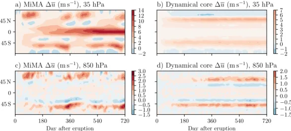
Figure 6 shows the evolution of the zonal wind re- sponses in two models at 35 hPa, through the core of the warming, and 850 hPa, an ideal level to track the extra- tropical eddy-driven jets. In MiMA (the configuration with the more realistic lower boundary conditions is shown), we see a relatively quick convergence of the extratropical stratosphere to the equilibrium, seasonally evolving response over a period of 2–3 months. The associated signal in the troposphere lags that of the stratosphere (very slightly in the NH but much more in the SH); however, quantifying the lag is complicated by the presence of the annual cycle. It does appear well converged within one year. These results imply that the extratropical atmosphere reaches the equilibrium state within the lifetime of the aerosol forcing (1–3 years),
although slow ocean feedbacks may play a role on lon- ger time scales in the real atmosphere.
The dynamical core simulations are easier to in- terpret, as they are run in perpetual boreal winter with no seasonal cycle. The lag of the tropospheric winds behind the extratropical stratospheric winds is readily apparent, particularly in the winter hemisphere (NH).
The simplified boundary conditions (and hence less in- ternal variability, particularly in the stratosphere) may also play a role in amplifying the tropospheric lag; re- sults in the MiMA configuration without topography (not shown) appear to show a greater tropospheric lag in comparison with the zonally asymmetric configuration.
We speculate that stationary waves tighten the dy- namical coupling between the troposphere and strato- sphere. They also impact the tropospheric variability directly, however, which could affect their sensitivity and response time.
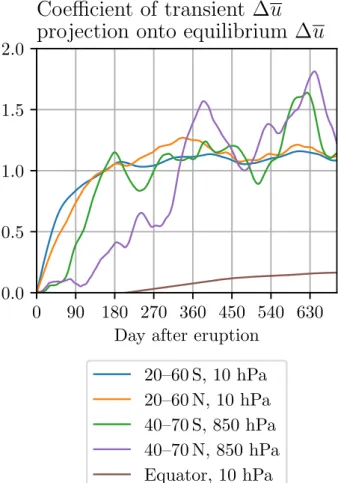
To quantify these results more precisely in the dy- namical core integrations, we project the transient zonal wind response as a function of time onto the equilibrium response (Fig. 7). Interpretation of the adjustment time is simpler for the dynamical core since it runs in per- petual January; applying the same metric in MiMA suffers from a lower signal-to-noise ratio and the com- plication of the annual cycle. We see that the stratosphere immediately begins adjustment toward equilibrium on a time scale of 1–2 months, but the tropospheric jets have little response for approximately 2 weeks and then con- verge on a slower time scale of 4–10 months. In both the
FIG. 6. Temporal evolution of the zonally averaged zonal wind response to warming, following a 1 Jan abrupt initiation of stratospheric warming in (a),(c) MiMA with zonal asymmetries and (b),(d) the dynamical core with a flat boundary. The response is defined as the difference between the ensemble mean of the switch on experiments less the mean of control integration, which evolves with the annual cycle in the case of MiMA. The levels 35 and 850 hPa are characteristic of the response of the stratospheric and tropospheric winds, respectively. The pairs of panels in (a) and (b) and in (c) and (d) each share a color scale, but a finer contour interval was used to show additional detail in the dynamical core integrations where the response was weaker.
stratosphere and the troposphere, the winter response is evidently slower than the summer response by roughly a factor of 2, despite winter and summer responses having similar magnitude. This is qualitatively opposite to the response in MiMA, emphasizing the role of stationary waves in setting the adjustment time scale.
We conclude that warming of the tropical stratosphere drives a rapid response in the extratropical stratosphere, while the tropospheric response converges on a longer time scale. This is consistent with a top-down mechanism, where the polar vortex modifies the eddy-driven jet as found with the annular mode response to sudden strato- spheric warmings (e.g., Baldwin and Dunkerton 2001)
that can operate in all seasons, and indeed, the response to ozone loss and recovery in the SH peaks in late spring to summer.
b. The slow tropical response
Figure 7hints at a possible ‘‘over-response’’ of the tropospheric circulation in the second year, where the overall projection exceeds the final climatological response. All curves will eventually asymptote to 1 by construction. Even with 100 ensemble members, however, there is still considerable internal variabil- ity, so we investigate this more closely.Figure 8bin- dicates that the second-year response in the winter hemisphere is larger than the equilibrium response, albeit with only marginal statistical confidence.
While the extratropical response of the circulation is largely on the time scale of weeks to months,Fig. 7 shows that the tropical stratosphere in the dynamical core requires a much longer time scale to adjust. The winds here ultimately require about a decade to fully converge. The slow evolution from tropical stratospheric easterlies to westerlies, shown inFigs. 8a and 8c, is asso- ciated with the adjustment time of the balanced response, which scales inversely with the Coriolis parameter (Holton et al. 1995). A decade is quite extreme—as stated below in the context of MiMA, the presence of an annual cycle limits the slow adjustment—but this is the region of the atmosphere that supports the QBO, which evolves on time scales orders of magnitude longer than the extratropical stratosphere.
Although the second year and steady-state responses at the equator are small and nearly equal at 35 hPa, they are large and of opposite sign at 10 hPa (Figs. 8a,c). The QBO-like difference in the stratosphere and small dif- ference in the jet is in rough quantitative agreement with the finding ofGarfinkel et al. (2012), who suggest that the QBO modifies the surface winds through the me- ridional circulation in the subtropics. In support of this mechanism, the extratropical stratospheric vortex is fairly well converged after one year, suggesting that it is not simply aHolton and Tan (1980)-type impact through the extratropical stratospheric vortex. Rather,
FIG. 7. The response of the zonal wind relative to the equilibrium (time mean) response, as a function of time, in the switch-on stratospheric warming experiments with the dynamical core, computed over specific regions as indicated in the legend. The relative response is determined by the coefficient of projection of the ensemble mean zonally averaged zonal wind response, pro- jected onto the equilibrium response and averaged over the specified regions; a value of 1 indicates that the ensemble mean response of the switch-on integrations has reached the equilibrium value at this level and latitudinal range. Projections are smoothed using a 30-day low-pass Butterworth filter and corrected for group delay to reduce the influence of natural variability.
the long-term evolution of the tropical stratosphere is associated with a slight decrease of the initial extra- tropical tropospheric response.
The tropical stratosphere also adjusts slowly in the configuration of MiMA without topography (not shown), although the addition of the annual cycle accelerates the process to some degree. The topographic configuration exhibits a faster tropical adjustment of a few years (Fig. 6), consistent with the time scale of the QBO. It is possible that volcanic eruptions may alter the QBO by modifying the dynamics of tropical wave activity, which can in turn impact the surface. This would still be possible within the 1–3-yr lifetime of stratospheric aerosol, and further in- vestigation may be possible with proposed model in- tercomparison projects with comprehensive models that can capture the QBO in a forced warming state.
c. Seasonality of the response
The lag in the tropospheric response, 1–3 months, is sufficiently long that the circulation may not reach an equilibrium at any point in the annual cycle. We con- sider in Fig. 9 the seasonality of the response using MiMA, which shows the composited transient response of zonal wind for the first 12 months after a 1 January
‘‘eruption’’ (i.e., an abrupt initiation of heating rate anomalies) in the flat configuration. Interpretation is
easier with this configuration of the model; as the re- sponse has essentially converged by the second half of the year, we can use June–December to observe the full response over a solstitial and equinoctial season, since the lower boundary is flat in both hemispheres.
The first few months show the initial response of the stratosphere; while a small tropospheric signal is present during this time, the contour intervals were chosen to em- phasize magnitudes larger than 1 m s22. The stratospheric response is initially more hemispherically symmetric (Jan- uary), whereas in just a few months (March) the presence of the winter vortex leads to amplified anomalies at height in the winter (boreal) hemisphere. The response at 100 hPa—
which is most critical for stratosphere–troposphere cou- pling—is remarkably similar in both hemispheres at all times of the year, and so appears to be connected with the essential response to warming in the lower stratosphere.
The response of the winds at height, which tends to dominate the picture, is largely dictated by the annual cycle of the vortices, which act as valves to planetary wave propagation into the middle and upper strato- sphere. At all times, the winds accelerate on the equa- torward flank of the vortex, peaking in amplitude at the very end of its life cycle in late spring as it shrinks toward the pole before vanishing (the vortex is long-lived in this configuration, given the lack of planetary wave forcing).
FIG. 8. Comparison of the equilibrium and second year response of the zonally averaged zonal wind to warming in the three-dimensional dynamical core (which runs in perpetual January). The equilibrium response is the difference between means of 100-yr steady in- tegrations (stratospheric heating minus the control), while the year 2 response is based on the ensemble mean of the second year in 100 switch-on experiments, less the control. Shaded regions indicate 1sof uncertainty.
This structure is associated with a concomitant equator- ward shift in the wave breaking and critical lines, which form along the edge of the vortex. While it is tempting to fall back on the thermal wind argument (where tropical warming increases the temperature gradient, accelerating the winds and bending waves equatorward), we stress that it is only valid a posteriori, requiring the nonlinear dy- namics of the three-dimensional models. The end result is consistent with wave refraction and wave driving argu- ments, but not easy to predict a priori.
The tropospheric response tends to maximize in sol- stitial seasons, weakening most notably in spring. For the solstitial seasons, the 1–3-month lag is sufficiently short for the circulation to fully spin up before the an- nual cycle changes the basic state. As seen inFigs. 2f and 2h, the situation is more complicated in the more re- alistic configuration of MiMA, and a boreal summer tropospheric response is notably absent, consistent with
findings from comprehensive models (e.g.,Barnes et al.
2016). The stratospheric evolution is similar in the more realistic configuration model, although the enhanced planetary wave activity shortens the lifetime of the polar vortices in the spring, further localizing the middle and upper stratospheric wind anomalies to the solstitial seasons (not shown). The shutdown of the QBO-like oscillation in this configuration admittedly complicates the analysis (essentially, reducing our effective sample size), but the early evolution of the extratropical re- sponse appears to be insensitive to the initial phase of the QBO.
7. Linking the response to volcanic forcing with the internal variability of the atmosphere
A number of studies have highlighted connections between the response to volcanic eruptions and the
FIG. 9. Monthly evolution of the zonally averaged zonal wind responses to warming in MiMA with a flat lower boundary, following a 1 Jan abrupt initiation of heating rate anomalies. Contoured for reference are the model’s climatological winds (in isotachs of 10 m s21, with easterly isotachs dashed and the zero isotach bolded).
annular modes of variability (e.g.,Perlwitz and Graf 1995;
Bittner et al. 2016b;Barnes et al. 2016;McGraw et al.
2016). The annular modes dominate variability in the ex- tratropical atmosphere in both hemispheres (Thompson and Wallace 2000) and have been linked to the response to external forcings, including greenhouse gases (e.g., Kushner et al. 2001) and stratospheric ozone (e.g., Son et al. 2010).Ring and Plumb (2007)highlight the fact that the annular mode seems to be a preferred response to external forcings, andGarfinkel et al. (2013)suggest that the annular modes can be used to quantify the strength and structure of eddy–vortex–jet interactions, which we have shown to be critical in understanding the circulation response to stratospheric warming.
As we have focused thus far on the response of the polar vortices and tropospheric jets, we examine the relation to natural variability by constructing the annu- lar modes from the zonal wind fields. A similar picture emerges if we use geopotential height, which is more commonly used to characterize the annular modes.
We define the annular mode index on each individual pressure level to be the leading principal component of 10-day low-pass-filtered daily zonal-mean zonal wind anomalies poleward of 308, latitude-weighted to account for sphericity. These anomalies are taken with respect to the control climatology, which evolves seasonally in the MiMA runs. The index is defined separately for the JJA and DJF seasons, allowing us to compare directly with pre-existing variability in that season. After normalizing the annular mode index to have unit variance, we obtain the annular mode patterns by regressing the original (unweighted) zonal-mean zonal winds onto the index.
With this convention, the annular mode pattern has physical units of meters per second and amplitude corresponding to one standard deviation of variability.
We compare the structure and amplitude of the circulation response to stratospheric warming in both MiMA and the dynamical core inTable 4. For the runs without topography, by symmetry we need only consider one solstice season (DJF). We report one stratospheric level, 35 hPa, which captures the variability and re- sponse of the polar vortex, and one tropospheric level, 850 hPa, which best captures the variability and response of the eddy-driven flow of the troposphere. The results are qualitatively similar for other levels within the strato- sphere and troposphere, respectively. The variance columns of Table 4 tabulate the fraction of variance captured by the annular mode in the control run. We see that the annular mode dominates the natural vari- ability of the zonal-mean zonal wind in all seasons at both levels. We now examine the pattern correlation rbetween these modes and the warming responses in the forced experiments, as well as the response ampli- tude A in units of one standard deviation of natural variability.
The first two rows ofTable 4compare the circula- tion response to stratospheric warming with the nat- ural variability in boreal winter in our more realistic configuration of MiMA. In the NH, the response nearly perfectly aligns with the annular mode struc- ture, with a pattern correlation close to unity at both 35 and 850 hPa. Relative to the natural variability, however, the NH response is comparatively weak, being equivalent to 0.47sin the stratosphere and even smaller (A85050:23s) in the troposphere. This weak signal is consistent with the difficulty of isolating the response in comprehensive models.
Under a difference of means test, the number of in- dependent samples required to reject the null hypothesis at 95% for a signal of this strength is 81. The annular
TABLE4. A comparison of the zonal wind response to stratospheric warming with natural variability, as represented by the annular modes, for different experiments (as listed inTable 2), seasons, and hemispheres. The columns VarianceXindicate the fraction of total variance captured by the annular mode at pressure levelX(35 and 850 hPa, indicative of stratospheric and tropospheric conditions, respectively); a large fraction here indicates that the natural variability is dominated by the annular mode, which is nearly always the case.
ColumnsrXindicate the spatial correlation between the annular mode and the response at pressure levelX; a value near unity indicates that the structure of the response to stratospheric warming is nearly identical to that of the annular mode. ColumnsAXshow the relative amplitude of the response compared to a 1 standard deviation amplitude of the annular mode; a value of unity indicates that the response is as large as a typical anomaly of the annular mode on daily time scales.
Experiments Season Hemisphere Variance35 r35 A35 Variance850 r850 A850
4 vs 1 (MiMA with zonal asymmetries) DJF SH 0.66 0.50 0.89 0.53 0.99 0.66
4 vs 1 (MiMA with zonal asymmetries) DJF NH 0.70 0.98 0.47 0.51 0.99 0.23
4 vs 1 (MiMA with zonal asymmetries) JJA SH 0.62 0.54 1.4 0.47 0.98 1.2
4 vs 1 (MiMA with zonal asymmetries) JJA NH 0.43 0.52 1.2 0.37 0.66 0.13
7 vs 6 (MiMA, flat) DJF SH 0.81 0.92 1.3 0.69 0.99 0.83
7 vs 6 (MiMA, flat) DJF NH 0.56 0.77 1.7 0.61 0.99 0.61
9 vs 8 (Dynamical core, flat) DJF SH 0.53 0.97 2.0 0.81 0.96 0.42
9 vs 8 (Dynamical core, flat) DJF NH 0.73 0.96 1.2 0.72 0.99 0.26
magnitude is halved. However, our forcing is strong rela- tive to observations of Pinatubo, so five samples may be an optimistic estimate.
One could also ask: How large of an eruption would be necessary to observe the surface wind response with 95% confidence? As seen in Fig. 5, the tropospheric response scales fairly linearly with the forcing. Doubling the warming of the stratosphere would thus cut the necessary sample size by roughly a factor of 4, so that we could expect to see the response in about two winters, and so one large eruption.
In the SH, the tropospheric response also aligns al- most perfectly with the natural variability (r85050:99), and compared to natural variability is 3 times as strong as in the NH. In the stratosphere, however, the response does not overlap very well with the structure of natural variability. In the austral winter, the SH response is re- markably similar: near-perfect alignment in the tropo- sphere (albeit weaker relative to natural variability), with a poorer overlap in the stratosphere. In the NH, the tropospheric response is less like the annular mode, consistent with the findings ofBarnes et al. (2016), who investigated more complex models.
The more idealized models are remarkably consistent with the results of MiMA’s realistic configuration: 1) the tropospheric response generally aligns very well with the annular mode variability, more so than the stratospheric response; 2) the response is weaker relative to the am- plitude of natural variability in the troposphere than the stratosphere; and 3) the winter response is generally smaller relative to natural variability than the summer response. We interpret these observations as follows:
1) The stratospheric response is influenced by the struc- ture of the warming perturbation and residual circula- tion response thereto (Toohey et al. 2014)—and so deviates from the structure of natural variability—
while the tropospheric response (at least in our models) is exclusively driven by the eddy coupling characterized by the annular mode.
2) The relative strength of the response in the strato- sphere is also consistent with the fact that the residual
circulation there is directly forced. The weaker tropo- spheric response matches the reduced amplitude of the tropospheric response to natural variability, such as sudden stratospheric warmings (e.g.,Baldwin and Dunkerton 2001).
3) The relative increase of the signal-to-noise ratio of the response in summer compared to winter is consis- tent with the relative lack of variability in the summer hemisphere. The stronger amplitude (in an absolute sense; seeFigs. 2f,h) also lines up with the enhanced temporal variability of the annular mode (Garfinkel et al. 2013).
By calling the consistency across models ‘‘remark- able,’’ we emphasize that the variability (and response) change dramatically across these integrations. The degree of consistency suggests a generic relationship between the response and variability. To illustrate this point,Fig. 10 shows two examples comparing a two-dimensional annular mode with the circulation response. Here, the annular mode overlays the NH DJF warming response in MiMA for both configurations previously described.
As shown in Fig. 7 ofGerber and Polvani (2009), the annular mode structure changes dramatically with the lower boundary conditions, shifting from a troposphere- dominated mode (Fig. 10b) to a stratosphere–troposphere coupled mode (Fig. 10a) with the addition of planetary wave forcings. This mirrors the difference between the
FIG. 10. The extratropical zonally averaged zonal wind responses to warming (shaded) and corresponding annular modes (contoured) for NH DJF in MiMA (a) with and (b) without zonal asymmetries in the lower boundary. The annular modes are contoured in isotachs of 1 m s21per unit variance, with easterly isotachs dashed and the zero isotach bolded. The change in the model’s boundary conditions shifts both the zonal wind response and the annular mode, particularly in the troposphere, and similarly modifies their vertical structure.